Chapter 10: Nonconjugate priors and Metropolis-Hastings algorithms

Jesse Mu

2016-12-08

1 Generalized linear models

Poisson + logistic. No conjugate priors.

2 Metropolis algorithm

s2 = 1; t2 = 10; mu = 5
y = c(9.37, 10.18, 9.16, 11.60, 10.33)
theta = 0
delta2 = 2
S = 10000
THETA = rep(NA, S)

set.seed(1)

# theta - current sample
# theta.star - proposed sample according to proposal distribution
# log.r - acceptance ratio
for (s in 1:S) {
  theta.star = rnorm(1, theta, sqrt(delta2))
  log.r = (sum(dnorm(y, theta.star, sqrt(s2), log = TRUE)) +
             dnorm(theta.star, mu, sqrt(t2), log = TRUE)) -
    (sum(dnorm(y, theta, sqrt(s2), log = TRUE)) +
       dnorm(theta, mu, sqrt(t2), log = TRUE))
  
  if (log(runif(1)) < log.r) theta = theta.star
  
  THETA[s] = theta
}

theta.df = data.frame(
  iteration = 1:S,
  theta = THETA
)
ggplot(theta.df, aes(x = iteration, y = theta)) +
  geom_line()

Interestingly, the effective sample sizes is quite low, only in the low thousands:

library(coda)
effectiveSize(THETA)
#>     var1 
#> 1427.451

acf(THETA)

real.df = data.frame(
  theta = seq(8, 12, length = 500),
  density = dnorm(seq(8, 12, length = 500), 10.03, .44)
)
ggplot(theta.df) +
  geom_histogram(aes(x = theta, y = ..density..), bins = 60) +
  geom_line(data = real.df, mapping = aes(x = theta, y = density))

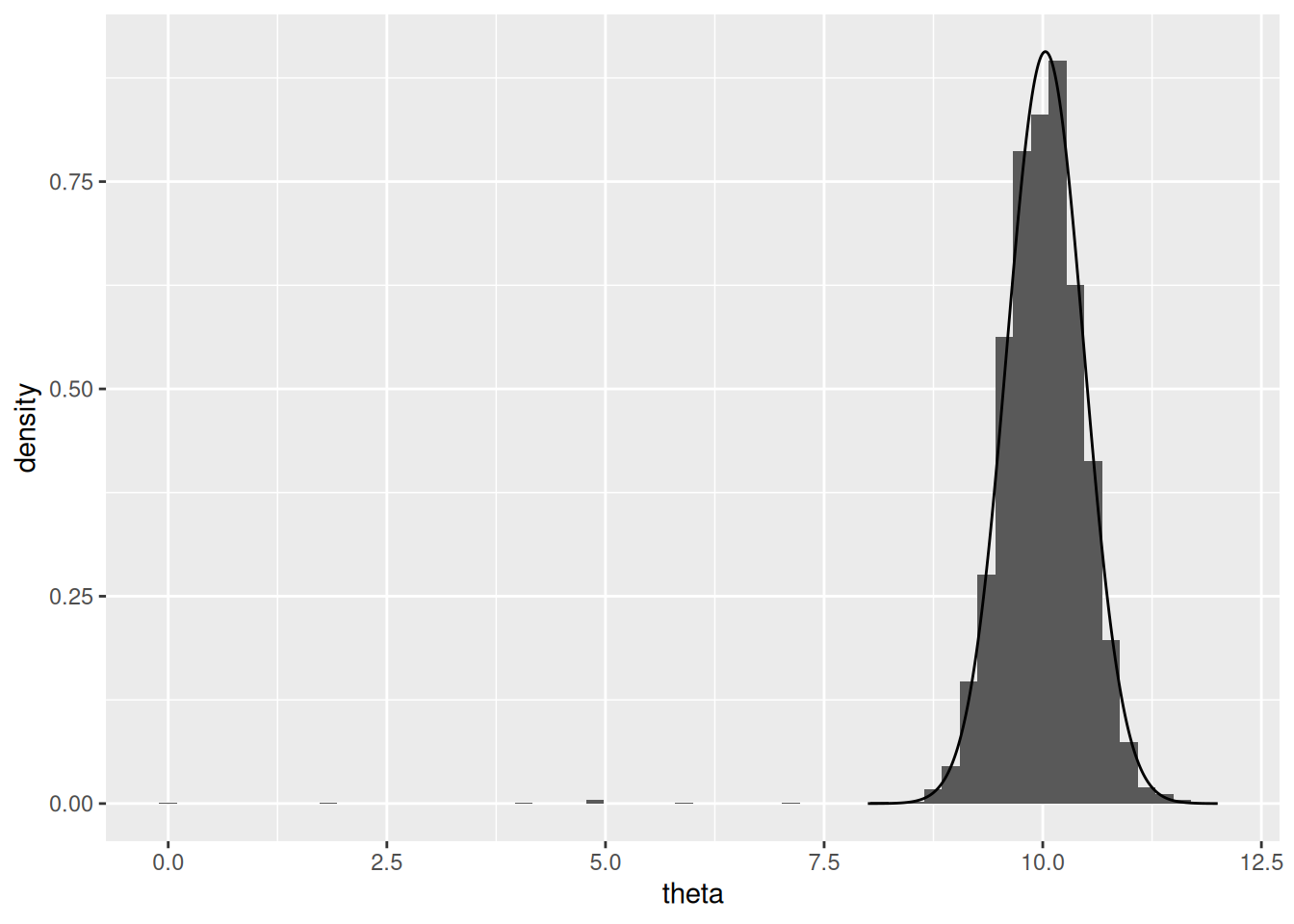
# outs[, 4]
# distribution looks different if we include 25000 vs ...  1000

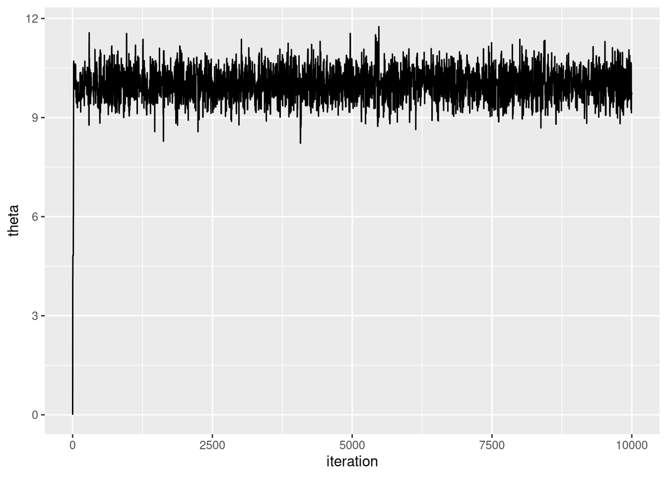
Output of the Metropolis algorithm

Need to run until stationarity

Different proposal distributions. Delta as a tradeoff between rate of approach towards the HPD region versus overshooting (like learning rate in gradient descent, etc)

Acceptance rate of between 20 and 50% is good. Control length

2.1 Combining Metropolis and Gibbs algorithms

Since proposal distributions for different parameters can all be different - could use Gibbs for some parameters (where Gibbs is just a special case of Metropolis-Hastings)

A regression model with correlated errors

This section explores running multiple independent MCMC chains and combining the data (which is theoretically OK). The approach in icecore_parallel.R is to take the MH algorithm for analyzing the icecore data and distribute it across multiple cores with parallel::mclapply. That file creates icecore_mcmc which is analyzed here.

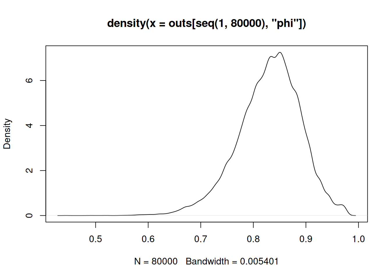
if (!file.exists('./icecore_mcmc')) {
  stop("Run icecore_parallel.R first to get MCMC data")
}
load('./icecore_mcmc')
# Should have "outs" now
# TODO: put colnames in icecore_parallel
colnames(outs) = c('b1', 'b2', 's2', 'phi')
plot(density(outs[seq(1, 80000), 'phi']))

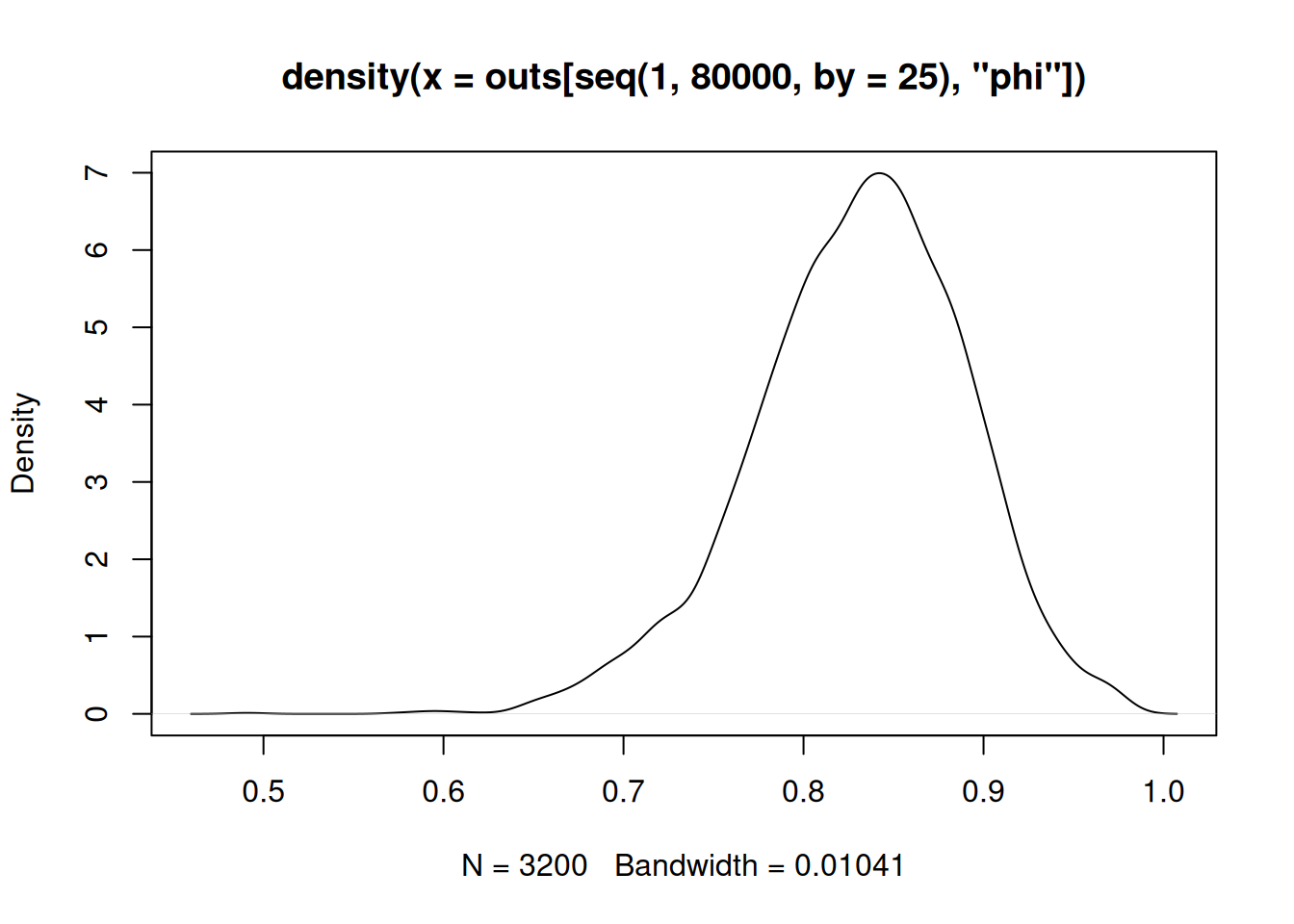
plot(density(outs[seq(1, 80000, by = 25), 'phi']))

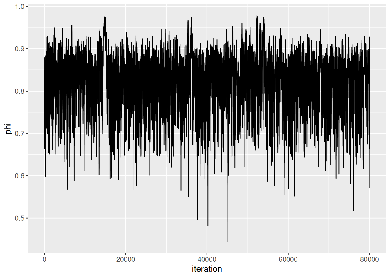
outs.df = data.frame(outs)
outs.df$iteration = 1:nrow(outs.df)

message(nrow(outs.df), " samples in ./icecore_mcmc")

ggplot(outs.df, aes(x = iteration, y = phi)) +
  geom_line()

effectiveSize(outs.df$phi)
#>     var1 
#> 1084.922

3 Exercises

3.1 10.2

msparrownest = read.table('Exercises/msparrownest.dat')

For convenience let \(\theta_i = P(Y_i = 1 \mid \alpha, \beta, x_i)\). Now we solve for \(\theta_i\) in our model

\[ \begin{aligned} & \log\left(\frac{\theta_i}{1 - \theta_i}\right) = \alpha + \beta x_i \\ \implies& \frac{\theta_i}{1 - \theta_i} = \exp(\alpha + \beta x_i) \\ \implies& \theta_i = \exp(\alpha + \beta x_i) - \theta_i \exp(\alpha + \beta x_i) \\ \implies& \theta_i = \frac{\exp(a + \beta x_i)}{1 + \exp(\alpha + \beta x_i)} \end{aligned} \]

So we know \(Y_i \sim \text{Bernoulli}\left(p_i\right)\) where \(p_i = \frac{\exp(a + \beta x_i)}{1 + \exp(a + \beta x_i)}\) and thus

\[ p(y_i \mid \alpha, \beta, x_i) = p_i^{y_i}(1 - p_i)^{1 - y_i} \]

a

Let \(z_i = \exp(\alpha + \beta x_i)\) for simplicity.

\[ \begin{aligned} p(\boldsymbol{y} \mid \alpha, \beta, x_i) &= \prod_{i = 1}^n p(y_i \mid \alpha, \beta, x_i) \\ &= \prod_{i = 1}^n p_i^{y_i} (1 - p_i)^{1 - y_i} \\ &= \prod_{i = 1}^n \left(\frac{z_i}{1 + z_i} \right)^{y_i} \left(1 - \frac{z_i}{1 + z_i} \right)^{1 - y_i} \\ &= \prod_{i = 1}^n \left(\frac{z_i}{1 + z_i} \right)^{y_i} \left(\frac{1 + z_i}{1 + z_i} - \frac{z_i}{1 + z_i} \right)^{1 - y_i} \\ &= \prod_{i = 1}^n \left(\frac{z_i}{1 + z_i} \right)^{y_i} \left(\frac{1}{1 + z_i}\right)^{1 - y_i} \\ &= \prod_{i = 1}^n \frac{z_i^{y_i}}{(1 + z_i)^{y_i}} \frac{1}{(1 + z_i)^{1 - y_i}} \\ &= \prod_{i = 1}^n \frac{z_i^{y_i}}{1 + z_i} \\ &= \prod_{i = 1}^n \frac{\exp(y_i (\alpha + \beta x_i))}{1 + \exp(\alpha + \beta x_i)} \\ \end{aligned} \]

and this cannot be simplified further.

b

It’s helpful to think about this in terms of the log-odds, i.e., \(\text{log-odds}(\theta_i) = a + \beta x_i\). With an uninformative prior where no interaction between wingspan \(x_i\) and nesting is assumed by default, the prior for \(\beta\) should be centered around 0. To also be uninformative about the prior proportion of nesting birds regardless of wingspan, the prior for \(\alpha\) should be centered around 0 as well, so the prior expectation regardless of \(x_i\) is \(\text{log-odds}(\theta_i) = 0 + 0 x_i = 0\) (thus not favoring nesting or not).

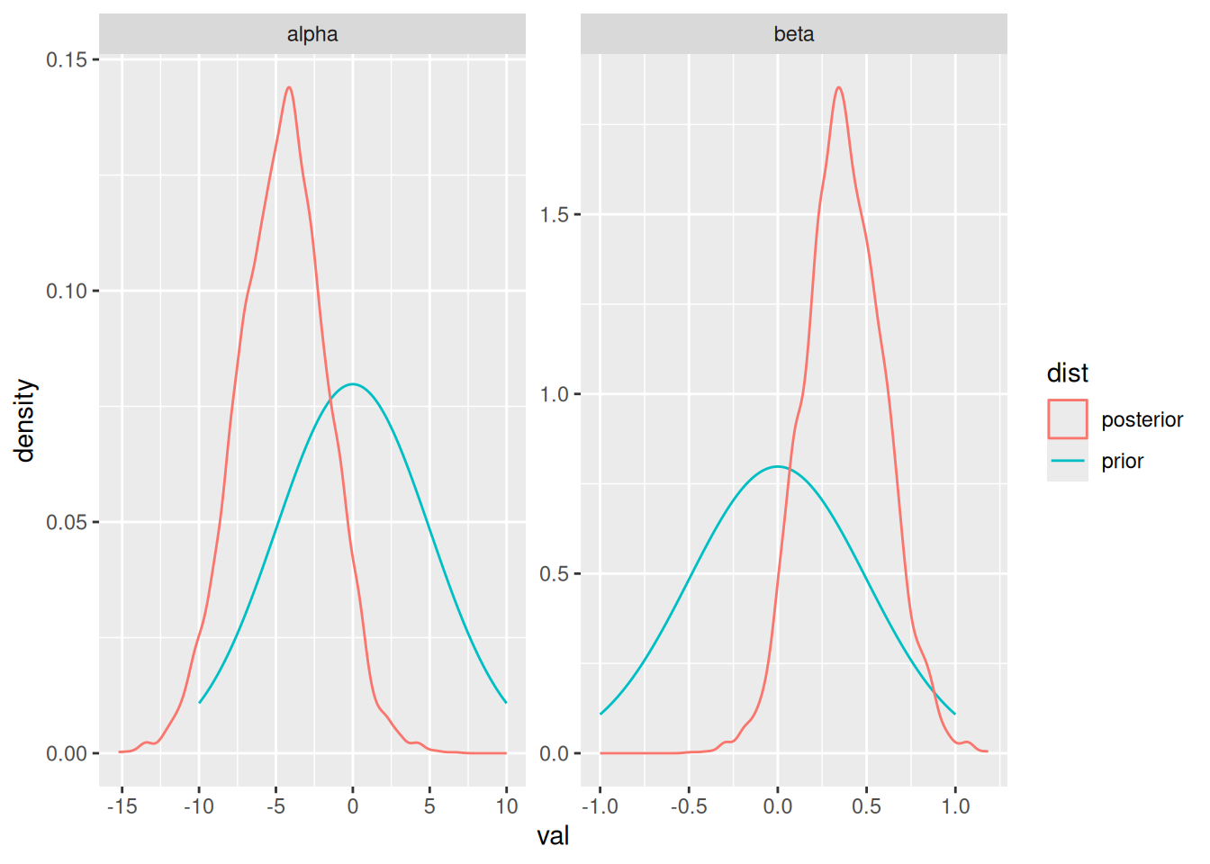
The question is what to use for a prior distribution and how diffuse to make the priors. Priors for \(\alpha\) and \(\beta\) should be symmetric, so normal distributions for both make sense. For an uninformative prior, the variance of these normals should be set high.

If \(\alpha\) is always 0, then as \(x\) moves from 10 to 15, the possible values of \(\beta\) should allow for a change in the log-odds ratio from approximately 0 to 1. Note the log-odds ratio of some sufficiently small number e.g. 1e-5 is -11.5129155 which is roughly 10. Since \(x\) at a minimum is 10, it makes sense to have most of the prior on \(\beta\) in the range \([-10 / 10, 10 / 10] = [-1, 1]\), so the standard deviation of the \(\beta\) prior is set to 0.5 and the variance to 0.25.

Similarly, the standard deviation of the \(\alpha\) prior to be 5 and the variance 25, so that, if \(\beta = 0\), the most of the \(\alpha\) prior falls in the log-odds interval \([-10, 10]\).

So

\[ \begin{aligned} \alpha &\sim \mathcal{N}(0, 25) \\ \beta &\sim \mathcal{N}(0, 0.25) \\ \end{aligned} \]

c

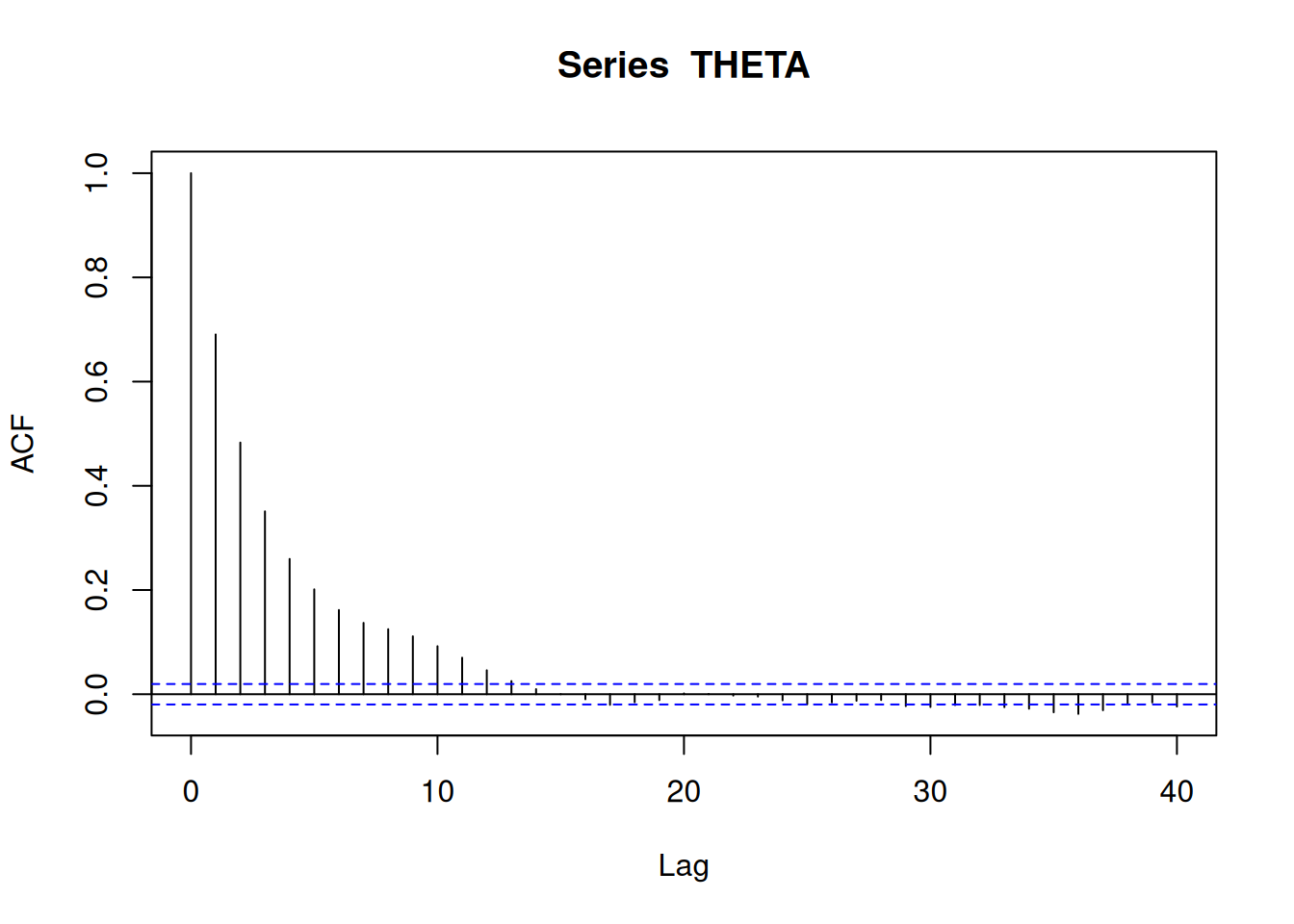
library(MASS)
inv = solve
# In this sampling scheme, when we sample, we keep the values together
# ($\theta$). But when I store the values, I split them (ALPHA, BETA).
S = 10000
burnin = 5000
y = msparrownest[, 1]
n = length(y)
# Use linear regression format, where column 1 is 1 (for alpha) and column 2 is
# the wingspan
x = cbind(rep(1, n), msparrownest[, 2])

# Start with X^T X but increase until acceptance ratio between 30% - 50%
var.prop = 7 * inv(t(x) %*% x)

# Prior parameters
pmn.theta = c(0, 0)
psd.theta = sqrt(c(25, 0.25))

# Where to store values
ALPHA = numeric(S + burnin)
BETA = numeric(S + burnin)
# Acceptances
acs = 0

# Initial estimates
theta = c(0, 0)

# For calculating likelihood ratio
log.p.y = function(x, y, theta) {
  exp_term = exp(x %*% theta)
  p = exp_term / (1 + exp_term)
  sum(dbinom(y, 1, p, log = TRUE))
}

p.theta = function(theta) {
  sum(dnorm(theta, pmn.theta, psd.theta, log = TRUE))
}

for (s in 1:(S + burnin)) {
  theta.star = mvrnorm(1, theta, var.prop)

  lhr = log.p.y(x, y, theta.star) +
    p.theta(theta.star) -
    log.p.y(x, y, theta) -
    p.theta(theta)

  if (log(runif(1)) < lhr) {
    theta = theta.star
    if (s > burnin) {
      acs = acs + 1
    }
  }
  ALPHA[s] = theta[1]
  BETA[s] = theta[2]
}
ALPHA = ALPHA[burnin:length(ALPHA)]
BETA = BETA[burnin:length(BETA)]

message("Acceptance ratio: ", acs / S) # Good to go
c(effectiveSize(ALPHA), effectiveSize(BETA))
#>     var1     var1 
#> 1569.255 1549.445

d

alpha_prior = data.frame(
  val = seq(-10, 10, length.out = 1000),
  density = dnorm(seq(-10, 10, length.out = 1000), 0, 5),
  var = 'alpha',
  dist = 'prior'
)
beta_prior = data.frame(
  val = seq(-1, 1, length.out = 1000),
  density = dnorm(seq(-1, 1, length.out = 1000), 0, 0.5),
  var = 'beta',
  dist = 'prior'
)
prior_df = rbind(alpha_prior, beta_prior)
alpha_post = data.frame(
  val = ALPHA,
  var = 'alpha',
  dist = 'posterior'
)
beta_post = data.frame(
  val = BETA,
  var = 'beta',
  dist = 'posterior'
)
post_df = rbind(alpha_post, beta_post)

ggplot(prior_df, aes(x = val, y = density, color = dist)) +
  geom_line() +
  geom_density(data = post_df, mapping = aes(x = val, y = ..density..)) +
  facet_wrap(~ var, scales = 'free')

e

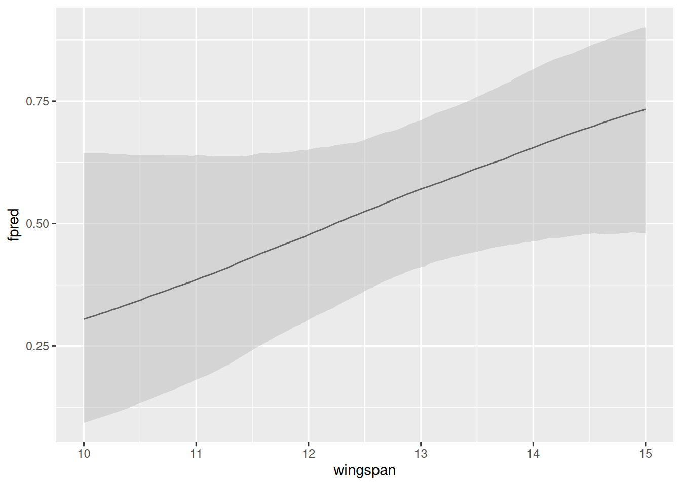
Using the samples of \(\alpha\) and \(\beta\), simply compute a distribution on \(f_{\alpha\beta}(x)\). Confidence intervals can then be constructed around this distribution. However, this needs to be done for many \(x\) values:

x_seq = seq(10, 15, length = 100)
quantiles = sapply(x_seq, function(x) {
  exp_term = exp(ALPHA + BETA * x)
  fab = exp_term / (1 + exp_term)
  quantile(fab, probs = c(0.025, 0.5, 0.975))
})

fab_df = data.frame(
  wingspan = x_seq,
  ymin = quantiles[1, ],
  fpred = quantiles[2, ],
  ymax = quantiles[3, ]
)

ggplot(fab_df, aes(x = wingspan, y = fpred, ymin = ymin, ymax = ymax)) +
  geom_line() +
  geom_ribbon(fill = 'grey', alpha = 0.5)

This is the logistic regressions’ approximate probability of nesting based on wingspan, although the confidence intervals are quite wide.