Unsupervised Learning Lab

Last modified: 2026-11-19

Show code
# The Python chunks on this page import matplotlib, numpy, pandas,
# scikit-learn and scipy; reticulate provisions them.
py_packages <- c("matplotlib", "numpy", "pandas", "scikit-learn", "scipy")
library(reticulate) # nolint: undesirable_function_linter
library(tidymodels) # nolint: undesirable_function_linter
py_require(py_packages)
1 The book’s Chapter 12 lab

This page holds the code lab for the Unsupervised Learning chapter.

To work the lab without the solutions, download a stub with only the exercises:

Each solution shows the code in Python and in R.

Section 12.5 of the book [1] is the source of these exercises. The Python code follows the book’s Chapter 12 lab notebook, with scikit-learn [2] in place of the ISLP package. The R code uses base R’s prcomp, kmeans and hclust.

2 Exploring the arrests data

Dataset 1: The arrests (USArrests) data

Arrest rates for violent crimes in 50 US states in 1973 make up the USArrests data [1, Sec. 12.5.1]. The data are in data/usarrests.csv, one row per state. The columns are:

  • Murder: murder arrests per \(100{,}000\) residents.
  • Assault: assault arrests per \(100{,}000\) residents.
  • Rape: rape arrests per \(100{,}000\) residents.
  • UrbanPop: the percentage of the state’s population that lives in cities.
Dataset 1: The arrests (USArrests) data

Exercise 1 (Lab: the scale of each arrest variable)

Exercise 1 (Lab: the scale of each arrest variable) Use the USArrests data. What are the sample mean and sample standard deviation of each of the four numeric variables?

Solution 1.

import pandas as pd

arr_eda_py = pd.read_csv("data/usarrests.csv")
arr_eda_py_cols = arr_eda_py[["Murder", "Assault", "UrbanPop", "Rape"]]
arr_eda_py_table = pd.DataFrame({
    "mean": arr_eda_py_cols.mean(),
    "sd": arr_eda_py_cols.std(),
})
arr_eda_py_table.round(1)
           mean    sd
Murder      7.8   4.4
Assault   170.8  83.3
UrbanPop   65.5  14.5
Rape       21.2   9.4
arr_eda_r <- readr::read_csv("data/usarrests.csv", show_col_types = FALSE)
arr_eda_r_cols <- select(arr_eda_r, Murder, Assault, UrbanPop, Rape)
arr_eda_r_names <- names(arr_eda_r_cols)
arr_eda_r_means <- map_dbl(arr_eda_r_cols, mean)
arr_eda_r_sds <- map_dbl(arr_eda_r_cols, sd)
arr_eda_r_table <- tibble(
  variable = arr_eda_r_names,
  mean = arr_eda_r_means,
  sd = arr_eda_r_sds
)
arr_eda_r_table

The variables are on very different scales: the standard deviation of Assault is 83.3, about 19 times the 4.4 of Murder. A method that compares the variables by their raw sizes would be dominated by Assault, which is the reason to standardize them before the next exercise.

Exercise 2 (Lab: murder and assault arrest rates)

Exercise 2 (Lab: murder and assault arrest rates) Use the USArrests data. What is the sample correlation between Murder and Assault?

Hint

Compute the correlation of two columns with a pandas method in Python, or with cor() in R.

Solution 2. This solution continues Solution 1.

arr_eda_py_cor = float(arr_eda_py["Murder"].corr(arr_eda_py["Assault"]))
round(arr_eda_py_cor, 3)
0.802
arr_eda_r_cor <- cor(arr_eda_r$Murder, arr_eda_r$Assault)
round(arr_eda_r_cor, 3)
[1] 0.802

The correlation is 0.8, so states with a higher murder arrest rate tend to have a higher assault arrest rate.

Exercise 3 (Lab: a histogram of murder arrest rates)

Exercise 3 (Lab: a histogram of murder arrest rates) Use the USArrests data. Draw a histogram of Murder.

Hint

Draw a histogram of one column, as in the histogram of the year of each car in the primer.

Solution 3. This solution continues Solution 2.

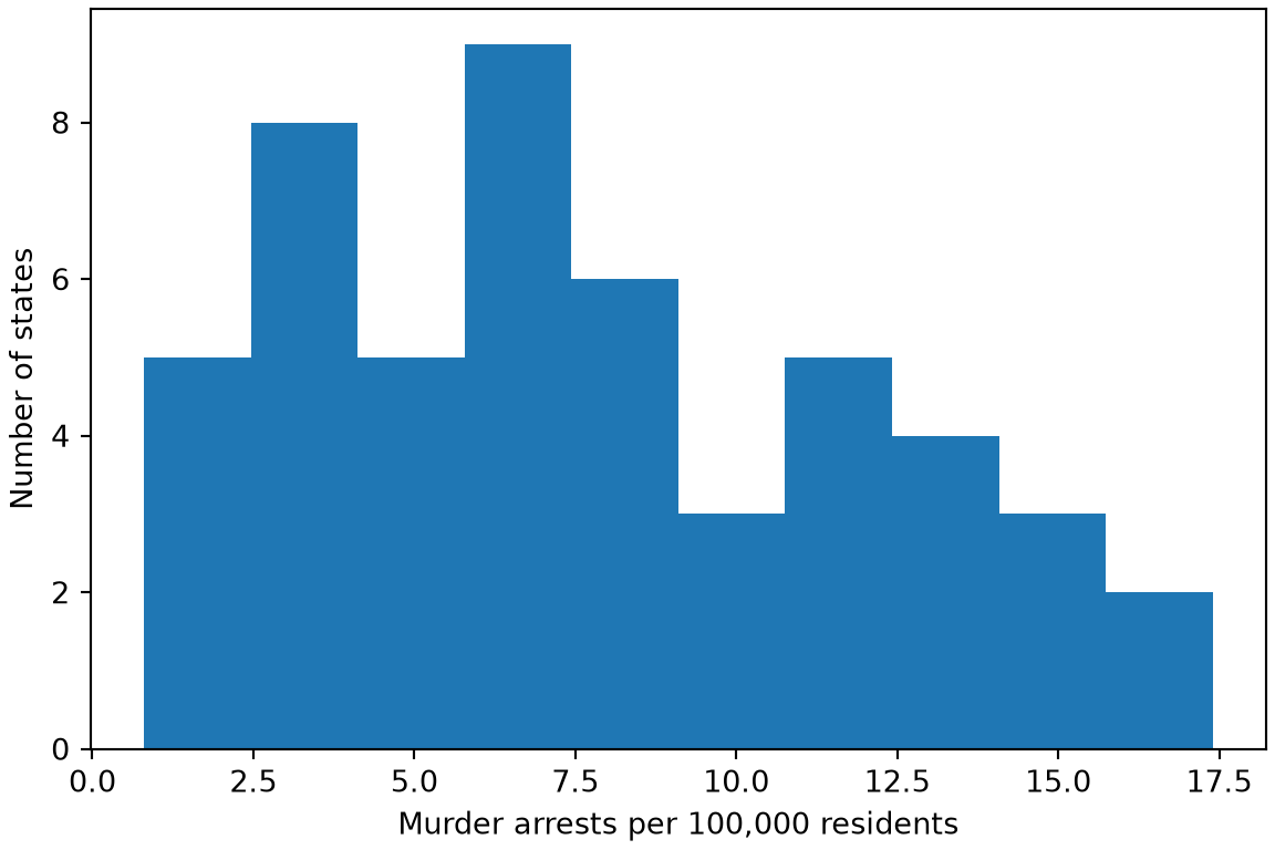
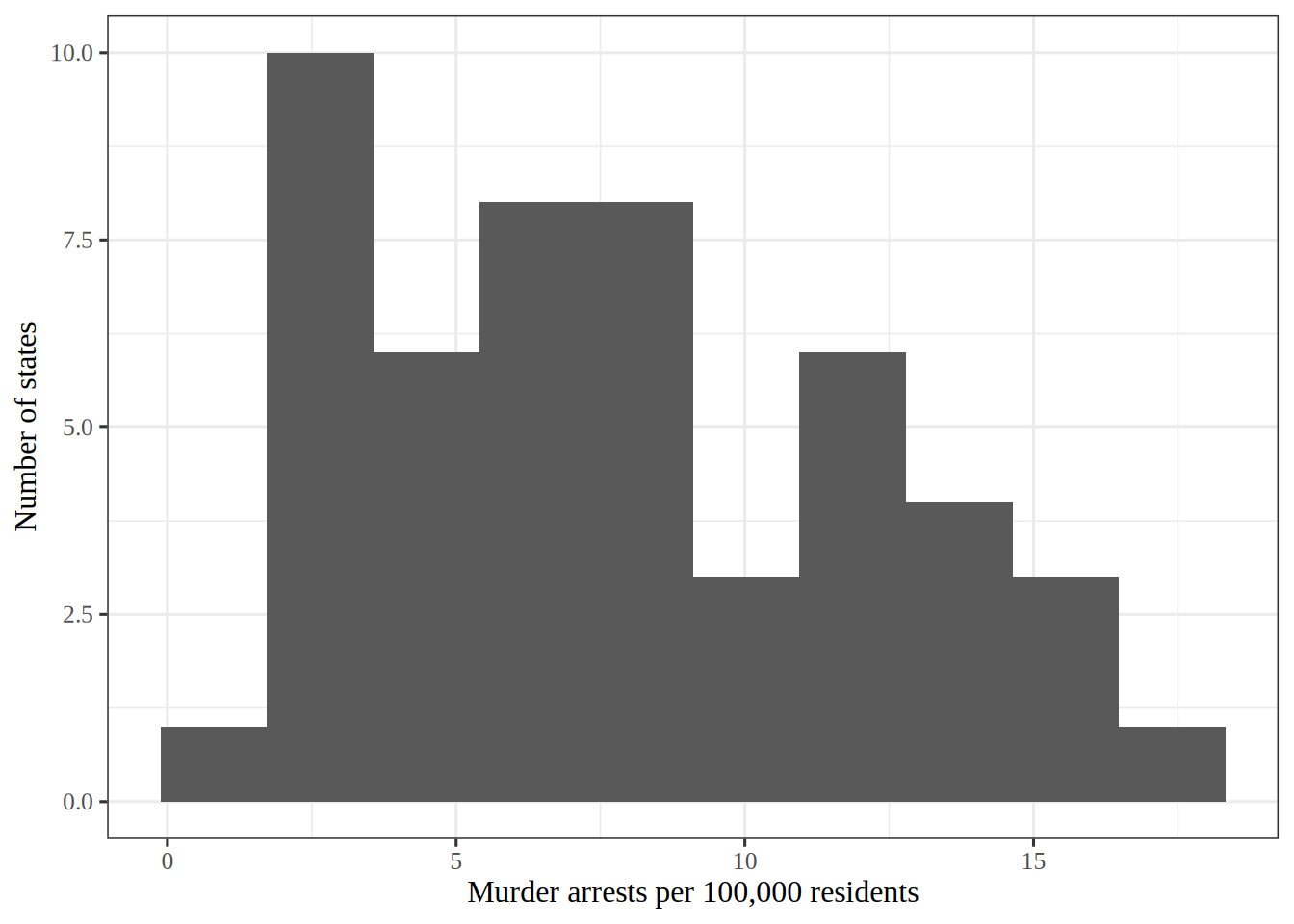
Figure 1: Bars counting the states at each level of murder arrests per 100,000 residents.
import matplotlib.pyplot as plt

fig, ax = plt.subplots(figsize=(6, 4), layout="constrained")
ax.hist(arr_eda_py["Murder"], bins=10);
ax.set_xlabel("Murder arrests per 100,000 residents");
ax.set_ylabel("Number of states");
plt.show()

Histogram of murder arrests per 100,000 residents in the 50 states, with the tallest bars at low and middle rates.

library(ggplot2) # nolint: undesirable_function_linter

murder_histogram <- arr_eda_r |>
  ggplot() +
  aes(Murder) +
  geom_histogram(bins = 10) +
  labs(x = "Murder arrests per 100,000 residents", y = "Number of states")
murder_histogram

Histogram of murder arrests per 100,000 residents in the 50 states, with the tallest bars at low and middle rates.

Show code
arr_eda_r_per_bin <- nrow(arr_eda_r) / 10

Figure 1 shows that most states have a low or middle number of murder arrests per 100,000 residents.

I chose 10 bins, which is 5 states per bar on average. Far fewer bins would hide the shape inside a few wide bars, and far more would leave most bars with one or two states, so the outline would look ragged. That is why 10 is a compromise between the two.

Exercise 4 (Lab: murder against assault arrest rates)

Exercise 4 (Lab: murder against assault arrest rates) Use the USArrests data. Draw a scatterplot of Murder against Assault.

Hint

Draw a scatterplot of one column against another, as in the plot of acceleration against horsepower in the primer.

Solution 4. This solution continues Solution 3.

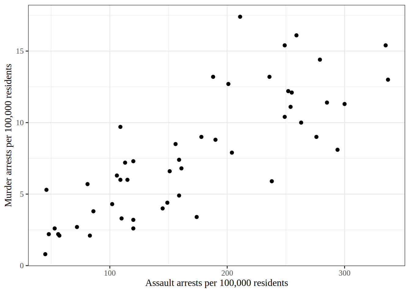
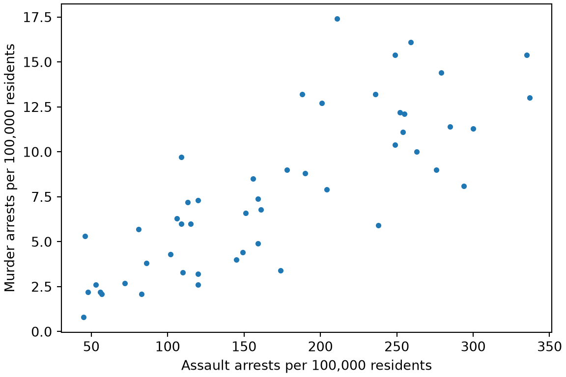
Figure 2: Murder arrests against assault arrests per 100,000 residents, with one dot per state.
fig, ax = plt.subplots(figsize=(6, 4), layout="constrained")
ax.scatter(arr_eda_py["Assault"], arr_eda_py["Murder"], s=10);
ax.set_xlabel("Assault arrests per 100,000 residents");
ax.set_ylabel("Murder arrests per 100,000 residents");
plt.show()

Scatterplot of murder arrests against assault arrests per 100,000 residents in the 50 states. The points rise from the lower left to the upper right along a band with some scatter around it.

murder_assault_plot <- arr_eda_r |>
  ggplot() +
  aes(Assault, Murder) +
  geom_point() +
  labs(
    x = "Assault arrests per 100,000 residents",
    y = "Murder arrests per 100,000 residents"
  )
murder_assault_plot

Scatterplot of murder arrests against assault arrests per 100,000 residents in the 50 states. The points rise from the lower left to the upper right along a band with some scatter around it.

Figure 2 shows murder arrests rising with assault arrests.

The points follow a rising band, which matches the positive correlation of the previous exercise. Because the two variables move together, a few directions in the plane carry most of the variation, and that is what principal components find.

3 Standardizing the variables

Exercise 5 (Lab: standardize the arrests data)

Exercise 5 (Lab: standardize the arrests data) Standardize the four variables of the USArrests data [1]: the murder, assault and rape arrest rates per \(100{,}000\) residents of each of the \(50\) US states, and the percentage of each state’s population that lives in cities.

Hint

A summary of each column gives its mean and standard deviation, and broadcasting subtracts and divides in one step to standardize every column.

Solution 5.

import pandas as pd
from sklearn.preprocessing import StandardScaler

arrests = pd.read_csv("data/usarrests.csv")
arrests_x = arrests[["Murder", "Assault", "UrbanPop", "Rape"]]
arrests_z = StandardScaler().fit_transform(arrests_x)
py_z_mean = float(abs(arrests_z.mean(axis=0)).max())
py_z_sd = arrests_z.std(axis=0)
py_z_sd
array([1., 1., 1., 1.])
arrests <- readr::read_csv("data/usarrests.csv", show_col_types = FALSE)
arrests_x <- select(arrests, Murder, Assault, UrbanPop, Rape)
arrests_z <- scale(arrests_x)
z_means <- colMeans(arrests_z)
arrests_z_tbl <- as_tibble(arrests_z)
r_z_sd <- map_dbl(arrests_z_tbl, sd)
r_z_sd
  Murder  Assault UrbanPop     Rape 
       1        1        1        1 

Each standardized variable should have mean \(0\) and standard deviation \(1\). The largest absolute column mean is 0 in the R run and 0 in the Python run. The smallest and largest standard deviations are 1 and 1 in the R run, whose scale divides by \(n - 1\). They are 1 and 1 in the Python run, whose StandardScaler divides by \(n\).

4 Principal components

Exercise 6 (Lab: find the first principal component)

Exercise 6 (Lab: find the first principal component) Find the first principal component of the standardized USArrests data from Exercise 5, and report its loading on each of the four variables.

The sign of a principal component is arbitrary, so the signs of the loadings can differ between libraries.

Hint

The linear algebra functions include the singular value decomposition and the eigendecomposition of a symmetric matrix, which are two routes to the principal components.

Solution 6.

from sklearn.decomposition import PCA

pca_py = PCA().fit(arrests_z)
pc1_py = pd.Series(pca_py.components_[0], index=arrests_x.columns)
pc1_py
Murder      0.535899
Assault     0.583184
UrbanPop    0.278191
Rape        0.543432
dtype: float64
arrests_pca <- prcomp(arrests_x, scale. = TRUE)
pc1_r <- arrests_pca$rotation[, 1]
pc1_r
    Murder    Assault   UrbanPop       Rape 
-0.5358995 -0.5831836 -0.2781909 -0.5434321 

The loadings of the first component have absolute values 0.54 on Murder, 0.58 on Assault, 0.28 on UrbanPop and 0.54 on Rape in the R run. The Python run gives 0.54, 0.58, 0.28 and 0.54.

Exercise 7 (Lab: find the proportion of variance explained)

Exercise 7 (Lab: find the proportion of variance explained) Find the proportion of the variance of the standardized USArrests data from Exercise 5 that each principal component explains.

Hint

The variance along each principal component comes from the singular values or eigenvalues of the linear algebra functions, as a share of their total.

Solution 7.

pve_py = pca_py.explained_variance_ratio_
pve_py
array([0.62006039, 0.24744129, 0.0891408 , 0.04335752])
pc_variances <- arrests_pca$sdev^2
pve_r <- pc_variances / sum(pc_variances)
pve_r
[1] 0.62006039 0.24744129 0.08914080 0.04335752

The first component explains 62% of the variance in the R run and 62% in the Python run. The second explains 24.7% in the R run and 24.7% in the Python run.

5 Clustering

Exercise 8 (Lab: cluster the states with k-means)

Exercise 8 (Lab: cluster the states with k-means) Cluster the standardized USArrests data from Exercise 5 into \(3\) groups with k-means, starting the algorithm from \(20\) random sets of centers and keeping the best result, and report the size of each cluster.

Hint

The KMeans estimator has a setting for the number of random starts, and its labels_ holds the cluster of each row. In R, kmeans() has an nstart setting for the number of random starts, and its cluster component holds the number of the group of each row.

Solution 8.

import numpy as np
from sklearn.cluster import KMeans

km_py = KMeans(n_clusters=3, n_init=20, random_state=0).fit(arrests_z)
km_sizes_py = np.sort(np.bincount(km_py.labels_))
km_sizes_py
array([14, 16, 20])
set.seed(571)
km_r <- kmeans(arrests_z, centers = 3, nstart = 20)
km_sizes_r <- sort(km_r$size)
km_sizes_r
[1] 13 17 20

The cluster sizes are 13, 17, 20 in the R run and 14, 16, 20 in the Python run. The numbering of the clusters is arbitrary, so the sizes are listed from smallest to largest. The two runs can disagree, because k-means finds a local optimum that depends on the random starting centers.

Exercise 9 (Lab: cluster the states hierarchically)

Exercise 9 (Lab: cluster the states hierarchically) Cluster the standardized USArrests data from Exercise 5 with complete linkage and Euclidean distance, cut the dendrogram into \(3\) clusters, and report the size of each cluster.

Hint

The linkage and fcluster functions build the merge tree and cut it into a chosen number of clusters. In R, hclust() builds the merge tree. Then cutree() cuts it.

Solution 9.

from scipy.cluster.hierarchy import fcluster, linkage

tree_py = linkage(arrests_z, method="complete", metric="euclidean")
hc_labels_py = fcluster(tree_py, t=3, criterion="maxclust")
hc_sizes_py = np.sort(np.bincount(hc_labels_py)[1:])
hc_sizes_py
array([ 8, 11, 31])
arrests_dist <- dist(arrests_z)
tree_r <- hclust(arrests_dist, method = "complete")
hc_labels_r <- cutree(tree_r, k = 3)
hc_counts_r <- table(hc_labels_r)
hc_sizes_r <- as.vector(hc_counts_r) |> sort()
hc_sizes_r
[1]  8 11 31

The cluster sizes are 8, 11, 31 in the R run and 8, 11, 31 in the Python run.

6 Gene expression data

Exercise 10 (Lab: find the principal components of gene expression)

Exercise 10 (Lab: find the principal components of gene expression) The NCI60 data [1] hold how active each of \(6830\) genes is in each of \(64\) cancer samples. Standardize each gene to have sample mean \(0\) and standard deviation \(1\), then compute the principal components of the samples. Report the proportion of the variance explained by each of the first \(5\) components.

Hint

Compute the principal components as in Exercise 6, with the linear algebra functions on the standardized matrix of samples by genes.

Solution 10.

import numpy as np
import pandas as pd
from sklearn.decomposition import PCA
from sklearn.preprocessing import StandardScaler

nci = pd.read_csv("data/nci60.csv")
nci_z_py = StandardScaler().fit_transform(nci.drop(columns="type"))
nci_pca_py = PCA().fit(nci_z_py)
nci_pve_py = nci_pca_py.explained_variance_ratio_[:5]
nci_pve_py.round(3)
array([0.114, 0.068, 0.058, 0.042, 0.037])
nci_r <- readr::read_csv("data/nci60.csv", show_col_types = FALSE)
nci_z <- scale(nci_r[names(nci_r) != "type"])
nci_pca <- prcomp(nci_z)
nci_variances <- nci_pca$sdev^2
nci_pve_r <- nci_variances / sum(nci_variances)
round(nci_pve_r[1:5], 3)
[1] 0.114 0.068 0.058 0.042 0.037

The first component explains 11.4% of the variance in the R run and 11.4% in the Python run. The first five together explain 31.8% in the R run and 31.8% in the Python run, so a few components carry a modest share of the information in \(6830\) genes.

Exercise 11 (Lab: cluster the samples hierarchically)

Exercise 11 (Lab: cluster the samples hierarchically) Cluster the standardized samples from Exercise 10 with complete linkage and Euclidean distance, cut the dendrogram into \(4\) clusters, and report the size of each cluster.

Hint

The linkage and fcluster functions build the merge tree and cut it into a chosen number of clusters, as in Exercise 9. In R, hclust() builds the merge tree. Then cutree() cuts it.

Solution 11.

import numpy as np
from scipy.cluster.hierarchy import fcluster, linkage

nci_tree_py = linkage(nci_z_py, method="complete", metric="euclidean")
nci_hc_py = fcluster(nci_tree_py, t=4, criterion="maxclust")
nci_hc_sizes_py = np.sort(np.bincount(nci_hc_py)[1:])
nci_hc_sizes_py
array([ 7,  8,  9, 40])
nci_dist <- dist(nci_z)
nci_tree <- hclust(nci_dist, method = "complete")
nci_hc_r <- cutree(nci_tree, k = 4)
nci_hc_counts <- table(nci_hc_r)
nci_hc_sizes_r <- as.vector(nci_hc_counts) |> sort()
nci_hc_sizes_r
[1]  7  8  9 40

The cluster sizes are 7, 8, 9, 40 in the R run and 7, 8, 9, 40 in the Python run.

Exercise 12 (Lab: cluster the samples with k-means)

Exercise 12 (Lab: cluster the samples with k-means) Cluster the standardized samples from Exercise 10 into \(4\) groups with k-means, starting the algorithm from \(20\) random sets of centers and keeping the best result, and report the size of each cluster.

Hint

The KMeans estimator has a setting for the number of random starts, and its labels_ holds the cluster of each row, as in Exercise 8. In R, kmeans() has an nstart setting for the number of random starts, and its cluster component holds the number of the group of each row.

Solution 12.

import numpy as np
from sklearn.cluster import KMeans

nci_km_py = KMeans(n_clusters=4, n_init=20, random_state=0).fit(nci_z_py)
nci_km_sizes_py = np.sort(np.bincount(nci_km_py.labels_))
nci_km_sizes_py
array([ 9,  9, 19, 27])
set.seed(1)
nci_km <- kmeans(nci_z, centers = 4, nstart = 20)
nci_km_sizes_r <- sort(nci_km$size)
nci_km_sizes_r
[1]  8  9 20 27

Exercise 13 (Lab: compare the k-means and hierarchical clusters)

Exercise 13 (Lab: compare the k-means and hierarchical clusters) Compare the sizes of the k-means clusters from Exercise 12 with the sizes of the hierarchical clusters from Exercise 11.

Hint

The counting functions tabulate each pair of values of two columns, here the two cluster assignments of each sample.

Solution 13. The k-means cluster sizes are 8, 9, 20, 27 in the R run and 9, 9, 19, 27 in the Python run, against 7, 8, 9, 40 and 7, 8, 9, 40 for the hierarchical clusters. Complete linkage puts 40 of the \(64\) samples in one cluster, while k-means spreads them more evenly. The k-means sizes can differ between the two runs, because k-means finds a local optimum that depends on its random starting centers.

References

[1]
G. James, D. Witten, T. Hastie, R. Tibshirani, and J. Taylor, An introduction to statistical learning: With applications in Python. Springer, 2023. doi: 10.1007/978-3-031-38747-0.
[2]
F. Pedregosa et al., “Scikit-learn: Machine learning in Python,” Journal of Machine Learning Research, vol. 12, pp. 2825–2830, 2011, Available: https://jmlr.org/papers/v12/pedregosa11a.html