Bias, Variance and Residual Variance

The bias-variance decomposition and how to read it

Last modified: 2026-11-19

Show code
# reticulate provisions the Python packages that this page imports.
library(reticulate) # nolint: undesirable_function_linter
py_packages <- c("numpy", "pandas", "matplotlib", "SyncRNG")
py_require(py_packages)

Source

Adapted from Brian Hutchinson’s Fall 2025 lecture notes, which supplied the crime-and-income example and the bias-variance decomposition. The contrast between stochastic and deterministic noise follows the treatment of overfitting in Abu-Mostafa et al. [1, Ch. 4]; the example and its numbers are new.

The bias-variance derivation is rewritten to assume only that the noise has mean zero, finite variance, and is independent of the training set, where the notes assumed it Gaussian; see Theorem 4. The wider reading is Hastie et al. [2], Chapter 2, and James et al. [3], Chapter 2.

1 Bias, variance and residual variance

Exercise 1 (What is random when a model predicts)

Exercise 1 (What is random when a model predicts) The Generalization page says the risk cannot be computed, only estimated. A different question about the same quantity is where it comes from: given a model that predicts badly, what are the distinguishable reasons it could be predicting badly?

Start with the pieces. Choose an input value \(x\), fit a model, and predict the output at \(x\). For that process, list each thing that is random.

Solution 1. Three things.

  • The output itself.
  • The training set \(\trainset\).
  • The fitted model \(\fitmodf{\trainset}\).

Exercise 2 (What is random when a model predicts (part 2))

Exercise 2 (What is random when a model predicts (part 2)) Use the setup of Exercise 1.

Say what makes each one random.

Solution 2.

  • The output itself. The world supplies a true mean function \(\truemean\) and noise: an input \(x\) has output \(Y = \truemeanf{x} + \noise\), where \(\noise\) is mean-zero noise independent of the training set (the noise model).

  • The training set \(\trainset\). It is a finite sample, and a different sample would have been just as possible.

  • The fitted model. The learning algorithm turns \(\trainset\) into a model, written \(\fitmodf{\trainset}\). Because \(\trainset\) is random, so is \(\fitmodf{\trainset}\).

Theorem 1 (The noise has population mean zero)

Theorem 1 (The noise has population mean zero) At any input \(\predvar\), the noise \(\noise\) has conditional expectation (population mean at \(\predvar\)) of \(0\):

\[ \condE{\noise}{\predvar} = 0 . \tag{1}\]

Proof

Proof. For the outcome \(\Outvar\) and noise \(\noise\) at input \(\predvar\), the true mean function value \(\truemeanf{\predvar}\) does not vary once \(\predvar\) is fixed, so its conditional expectation given \(\predvar\) is \(\truemeanf{\predvar}\).

\[ \begin{aligned} \condE{\noise}{\predvar} &= \condE{\Outvar - \truemeanf{\predvar}}{\predvar} && \text{(definition of the noise)} \\ &= \condE{\Outvar}{\predvar} - \truemeanf{\predvar} && \text{(linearity of expectation)} \\ &= \truemeanf{\predvar} - \truemeanf{\predvar} && \text{(definition of the true mean function)} \\ &= 0 && \text{(a number minus itself is zero)} . \end{aligned} \]

Example 1 (Noise in a count outcome)

Example 1 (Noise in a count outcome) Suppose the outcome \(\Outvar\) at input \(\predvar\) is a count with a Poisson distribution whose population mean is the true mean function value \(\truemeanf{\predvar}\). The noise \(\noise = \Outvar - \truemeanf{\predvar}\) has population mean \(0\), by Theorem 1. The variance of \(\noise\) at \(\predvar\) is \(\Var{\noise} = \truemeanf{\predvar}\), so the noise has larger variance at an input \(\predvar\) where \(\truemeanf{\predvar}\) is larger. The distribution of \(\noise\) at \(\predvar\) is also skewed: \(\noise\) cannot fall below \(-\truemeanf{\predvar}\) and has no upper bound. A gamma outcome behaves the same way: the noise is skewed, and the noise variance grows with the population mean \(\truemeanf{\predvar}\).

Example 2 (Noise in a binary outcome)

Example 2 (Noise in a binary outcome) Suppose the outcome \(\Outvar\) at input \(\predvar\) takes only the values \(0\) and \(1\), with a Bernoulli distribution whose population mean is the true mean function value \(\truemeanf{\predvar}\). That value is also the probability that \(\Outvar = 1\). The noise \(\noise = \Outvar - \truemeanf{\predvar}\) then takes only two values:

  • \(1 - \truemeanf{\predvar}\) when \(\Outvar = 1\), which has probability \(\truemeanf{\predvar}\);
  • \(-\truemeanf{\predvar}\) when \(\Outvar = 0\), which has probability \(1 - \truemeanf{\predvar}\).

The noise has population mean \(0\), by Theorem 1. At a fixed input \(\predvar\), the value \(\truemeanf{\predvar}\) is a constant, so \(\noise\) and \(\Outvar\) have the same variance. For a Bernoulli outcome, that variance is

\[ \Var{\noise} = \truemeanf{\predvar} \devof{1}{\truemeanf{\predvar}} . \]

The variance is largest at an input where \(\truemeanf{\predvar} = 1/2\), and it shrinks toward \(0\) as \(\truemeanf{\predvar}\) nears \(0\) or \(1\). So the two values the noise can take, and its variance, both depend on \(\truemeanf{\predvar}\). Wherever \(\truemeanf{\predvar}\) differs between inputs, the outcome is not its mean plus noise with the same cumulative distribution function at every input. Figure 1 draws the two noise values and the variance against \(\truemeanf{\predvar}\).

Show code
nb_colours <- c(
  "noise when outcome is 1" = "#0072B2",
  "noise when outcome is 0" = "#D55E00",
  "noise variance" = "black"
)
nb_linetypes <- c(
  "noise when outcome is 1" = "solid",
  "noise when outcome is 0" = "dashed",
  "noise variance" = "dotted"
)
nb_levels <- names(nb_colours)
nb_grid <- seq(0, 1, length.out = 101)
nb_curves <- tibble::tibble(mean = nb_grid) |>
  dplyr::mutate(
    `noise when outcome is 1` = 1 - mean,
    `noise when outcome is 0` = -mean,
    `noise variance` = mean * (1 - mean)
  ) |>
  tidyr::pivot_longer(-mean, names_to = "curve", values_to = "value") |>
  dplyr::mutate(curve = factor(curve, levels = nb_levels))
nb_curves |>
  ggplot2::ggplot() +
  ggplot2::aes(x = mean, y = value, colour = curve, linetype = curve) +
  ggplot2::geom_line(linewidth = 1) +
  ggplot2::scale_colour_manual(values = nb_colours) +
  ggplot2::scale_linetype_manual(values = nb_linetypes) +
  ggplot2::labs(
    x = "True mean function value",
    y = "Value",
    colour = NULL,
    linetype = NULL
  ) +
  ggplot2::theme(legend.position = "bottom")
Show code
import matplotlib.pyplot as plt
import numpy as np

nb_mean = np.linspace(0, 1, 101)
fig, ax = plt.subplots(figsize=(7, 4), layout="constrained")
ax.plot(nb_mean, 1 - nb_mean, color="#0072B2", linestyle="-", label="noise when outcome is 1");
ax.plot(nb_mean, -nb_mean, color="#D55E00", linestyle="--", label="noise when outcome is 0");
ax.plot(nb_mean, nb_mean * (1 - nb_mean), color="black", linestyle=":", label="noise variance");
ax.set_xlabel("True mean function value");
ax.set_ylabel("Value");
ax.legend(loc="lower left");
plt.show()
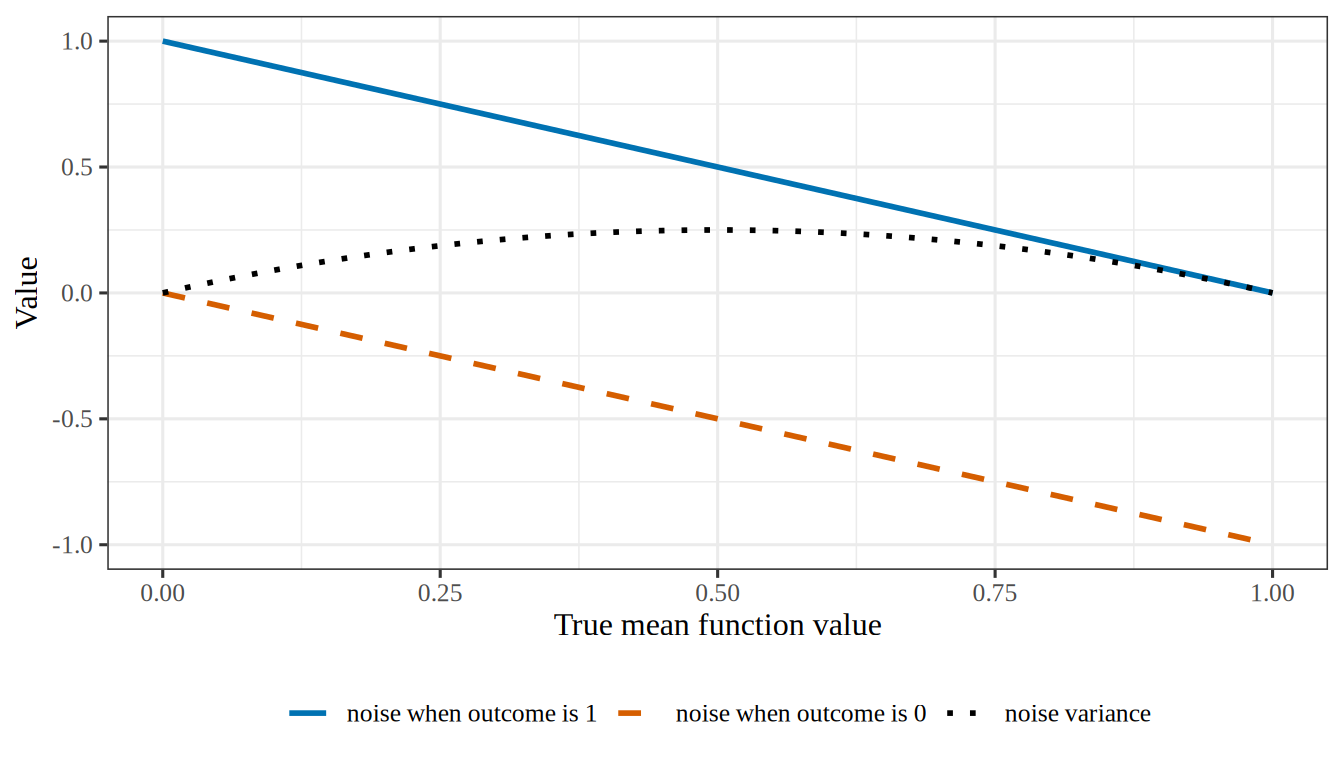
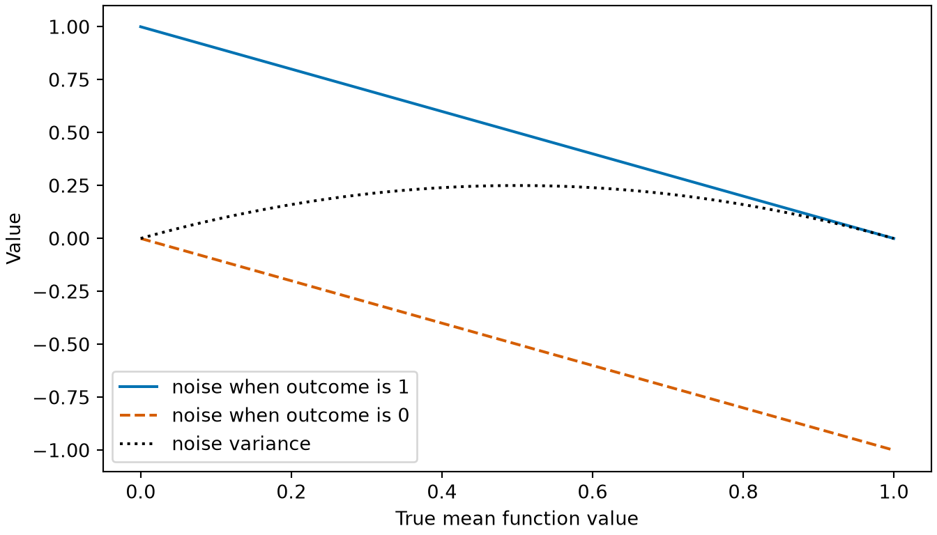
Figure 1: The two values the noise of a binary outcome can take, and the noise variance, as functions of the true mean function value at an input (Example 2).
(a)
A line plot against the true mean function value, from 0 to 1 on the horizontal axis. A solid blue line, the noise when the outcome is 1, falls from 1 to 0. A dashed vermilion line, the noise when the outcome is 0, falls from 0 to minus 1. A dotted black curve, the noise variance, is an arch that starts at 0, peaks at 0.25 where the true mean function value is 0.5, and returns to 0.
(b)
A line plot against the true mean function value, from 0 to 1 on the horizontal axis. A solid blue line, the noise when the outcome is 1, falls from 1 to 0. A dashed vermilion line, the noise when the outcome is 0, falls from 0 to minus 1. A dotted black curve, the noise variance, is an arch that starts at 0, peaks at 0.25 where the true mean function value is 0.5, and returns to 0.

Remark 1 (The noise can depend on the input)

Remark 1 (The noise can depend on the input). The distribution of the noise \(\noise\) at an input \(\predvar\) can change with \(\predvar\) (Example 1). That distribution can be skewed, and the variance of \(\noise\) need not be the same at every input. Only the population mean of \(\noise\) at \(\predvar\) must be zero (Theorem 1).

Remark 2 (The noise depends on which inputs it is conditional on)

Remark 2 (The noise depends on which inputs it is conditional on). The noise is defined only once the inputs in \(\predvar\) are chosen, as the statistics notes also say. Adding a feature to \(\predvar\) can change the true mean function, and with it the noise of the same observation.

Remark 3 (Independent noise draws across observations)

Remark 3 (Independent noise draws across observations). The noise \(\noise\) is a fresh random draw each time an outcome \(\Outvar\) is observed. Each outcome \(\Outvar_i\) in the training set \(\trainset\) at input \(\predvar_i\) is \(\Outvar_i = \truemeanf{\predvar_i} + \noise_i\), with true mean function value \(\truemeanf{\predvar_i}\) and noise draw \(\noise_i\), and a new outcome \(\Outvar\) at \(\predvar\) has a new draw \(\noise\). Once the inputs are fixed, \(\noise_i = \Outvar_i - \truemeanf{\predvar_i}\) and \(\noise = \Outvar - \truemeanf{\predvar}\) shift the outcomes by the fixed values \(\truemeanf{\predvar_i}\) and \(\truemeanf{\predvar}\), so conditional independence of the outcomes given the inputs is equivalent to conditional independence of the noise draws given the inputs. Under that conditional independence, when the distribution of \(\noise\) given \(\predvar\) does not change with \(\predvar\), the noise draws are independent of the inputs and of one another. When the distribution of \(\noise\) given \(\predvar\) changes with \(\predvar\) (Remark 1), a new observation drawn independently of \(\trainset\) still has a new draw \(\noise\) at the fixed input \(\predvar\) that is independent of \(\trainset\).

Remark 4 (The noise model in the probability notes)

Remark 4 (The noise model in the probability notes). For a single observation of the outcome \(\Outvar\) at input \(\predvar\) with true mean function value \(\truemeanf{\predvar}\) and a finite variance \(\varpar\), the noise model equation is a consequence of the definition of noise (\(\Outvar = \truemeanf{\predvar} + \noise\) for the noise \(\noise\)) and Theorem 1 (conditional expectation \(\condE{\noise}{\predvar} = 0\)), not an additional assumption. Only the noise’s population mean and variance matter here. The variance \(\varpar\) is the variance of \(\noise\) at the input \(\predvar\) under discussion, and that variance can change with \(\predvar\) (Remark 1). The probability notes call the noise model equation the mean-zero noise model.

The noise model fixes only two parts of a distribution model for the outcome: the mean function is \(\truemeanf{\predvar}\), and the variance is \(\varpar\). Any distribution model with that mean function and that variance satisfies the noise model, such as the normal distribution model with mean function \(\truemeanf{\predvar}\) and variance \(\varpar\).

Definition 1 (Prediction rule )

Definition 1 (Prediction rule ) A prediction rule is a fitted model \(\fitmodf{\trainset}\) that is used to predict the outcome at a new covariate value \(\predvar\). Its prediction is \(\predvalf{\predvar}\).

In words, the prediction rule takes a new covariate value and returns the fitted model’s value there.

See prediction rule in the statistics notes.

Example 3 (The fitted line as a prediction rule )

Example 3 (The fitted line as a prediction rule ) Take the line \(\fitmodf{\trainset}\) fitted to the five neighborhoods of the crime data, as in the fitted-line example. Using it to predict the crime rate of a sixth neighborhood makes it a prediction rule. Using the same line only to describe the five neighborhoods makes no prediction, so there it is a fitted model and not a prediction rule.

Definition 2 (Average fit)

Definition 2 (Average fit) The average fit at \(\predvar\) is the prediction \(\predvalf{\predvar}\) of the fitted model at \(\predvar\), averaged over every training set \(\trainset\) it might have been fitted to, where \(\Ep_{\trainset}\) denotes that average over training sets. It is the population expectation \[ \avgfitf{\predvar} \eqdef \Epredvalf{\predvar} , \tag{2}\] a fixed function of \(\predvar\) that nothing estimates, so it carries no hat. It is written like the true mean function, with the model as the subscript.

Example 4 (The average fit of a line on cylinders)

Example 4 (The average fit of a line on cylinders) Treat the 392 cars of the Auto data [3] as the whole world of cars. A training set is 30 cars drawn at random from it, and the learning algorithm fits the line of mpg on cylinders. Draw 2000 training sets, fit a line to each, and record each line’s intercept, slope and prediction at 4 cylinders. Both tabs draw with the SyncRNG package [4], a random number generator with the same algorithm in R and Python, from the same seed, so they pick the same cars:

Show code
import numpy as np
import pandas as pd
from SyncRNG import SyncRNG

auto_af = pd.read_csv("data/auto.csv").dropna(subset=["horsepower"])
cyl_af = auto_af["cylinders"].to_numpy(float)
mpg_af = auto_af["mpg"].to_numpy(float)

rng_af = SyncRNG(seed=1)
coefs_af = np.empty((2000, 2))
for s_af in range(2000):
    # One training set: the first 30 rows of a shuffle of all the rows (Python counts from 0), and the line fitted to it.
    pick_af = rng_af.shuffle(list(range(len(mpg_af))))[:30]
    slope_af, intercept_af = np.polyfit(cyl_af[pick_af], mpg_af[pick_af], 1)
    coefs_af[s_af] = intercept_af, slope_af

preds_af = coefs_af[:, 0] + coefs_af[:, 1] * 4

# The average fit at 4 cylinders is the mean of those predictions.
# The Monte Carlo standard error of that mean is the spread of the predictions over sqrt(2000).
mc_se_af = preds_af.std(ddof=1) / np.sqrt(2000)
print(preds_af.mean().round(2), preds_af.min().round(2), preds_af.max().round(2), mc_se_af.round(3))
28.72 23.89 32.74 0.031
Show code
auto_af <- read.csv("data/auto.csv")
auto_af <- na.omit(auto_af[, c("mpg", "cylinders", "horsepower")])

# SyncRNG is a random number generator with the same algorithm in R and Python, so the draws match the Python tab.
library(SyncRNG)
rng_af <- SyncRNG(seed = 1)
coefs_af <- t(replicate(2000, {
  # One training set: the first 30 rows of a shuffle of all the rows, and the line fitted to it.
  rows <- rng_af$shuffle(seq_len(nrow(auto_af)))[1:30]
  coef(lm(mpg ~ cylinders, data = auto_af[rows, ]))
}))

preds_af <- coefs_af[, 1] + coefs_af[, 2] * 4

# The average fit at 4 cylinders is the mean of those predictions.
# The Monte Carlo standard error of that mean is the spread of the predictions over sqrt(2000).
mc_se_af <- sd(preds_af) / sqrt(2000)
c(round(c(mean = mean(preds_af), min = min(preds_af), max = max(preds_af)), 2), mc_se = round(mc_se_af, 3))
  mean    min    max  mc_se 
28.720 23.890 32.740  0.031 

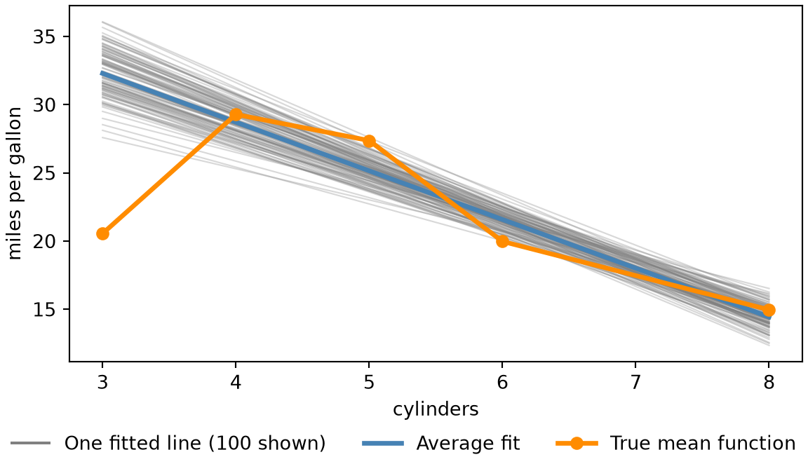
No single training set produces the average fit. The 2000 lines predict anywhere from 23.9 to 32.7 miles per gallon for a four-cylinder car, and their mean, 28.7, is the average fit \(\avgfitf{4}\) of Equation 2, with a 95% Monte Carlo confidence interval of 28.66 to 28.78 (1.96 Monte Carlo standard errors either side). The two tabs print the same numbers up to rounding.

Figure 2 plots 100 of the 2000 lines, their pointwise average, and the true mean function:

Show code
import numpy as np
import matplotlib.pyplot as plt

grid_af = np.arange(3, 9)
# The pointwise average fit is the mean of the fitted lines at each cylinder count.
avg_af = (coefs_af[:, [0]] + coefs_af[:, [1]] * grid_af).mean(axis=0)
# The true mean function is the mean mpg of the cars with each cylinder count.
truth_af = auto_af.groupby("cylinders")["mpg"].mean()

fig, ax = plt.subplots(figsize=(6, 3.5), layout="constrained")
for intercept_af, slope_af in coefs_af[:100]:
    ax.plot(grid_af, intercept_af + slope_af * grid_af, color="grey", alpha=0.3, linewidth=0.8);
# One legend entry for the 100 grey lines, with a solid line to stand for them.
ax.plot([], [], color="grey", label="One fitted line (100 shown)");
ax.plot(grid_af, avg_af, color="steelblue", linewidth=2.5, label="Average fit");
ax.plot(truth_af.index, truth_af.values, color="darkorange", linewidth=2.5, marker="o", label="True mean function");
ax.set_xlabel("cylinders");
ax.set_ylabel("miles per gallon");
fig.legend(loc="outside lower center", ncol=3, frameon=False);
plt.show()
Figure 2: The fitted lines of 100 of the 2000 training sets (grey), their pointwise average fit (blue), and the true mean function (orange), for mpg against cylinders.
A plot of miles per gallon against cylinders, from 3 to 8. One hundred faint grey lines slope downward and fan out, most widely at 3 and 8 cylinders and most narrowly between 6 and 7 cylinders. A thick blue line, the average of all 2000 fitted lines, runs down through the middle of the grey lines. A thick orange line with points at 3, 4, 5, 6 and 8 cylinders, the mean mpg of the cars with that many cylinders, is not straight: it starts well below the blue line at 3 cylinders, rises above it at 4 and 5, and then follows it down to 8. A legend below the plot names the three: one fitted line, average fit, and true mean function.
Show code
library(ggplot2)

grid_af <- 3:8
# One row per fitted line and cylinder count; the pointwise average fit is the mean over lines.
lines_af <- data.frame(
  line = rep(seq_len(nrow(coefs_af)), each = length(grid_af)),
  cylinders = grid_af,
  fit = as.vector(t(coefs_af[, 1] + outer(coefs_af[, 2], grid_af)))
)
avg_af <- aggregate(fit ~ cylinders, data = lines_af, FUN = mean)
# The true mean function is the mean mpg of the cars with each cylinder count.
truth_af <- aggregate(mpg ~ cylinders, data = auto_af, FUN = mean)

ggplot() +
  geom_line(data = subset(lines_af, line <= 100), aes(cylinders, fit, group = line, colour = "One fitted line (100 shown)"), alpha = 0.3) +
  geom_line(data = avg_af, aes(cylinders, fit, colour = "Average fit"), linewidth = 1.5) +
  geom_line(data = truth_af, aes(cylinders, mpg, colour = "True mean function"), linewidth = 1.5) +
  geom_point(data = truth_af, aes(cylinders, mpg, colour = "True mean function"), size = 3) +
  scale_colour_manual(
    values = c("One fitted line (100 shown)" = "grey60", "Average fit" = "steelblue", "True mean function" = "darkorange"),
    breaks = c("One fitted line (100 shown)", "Average fit", "True mean function")
  ) +
  guides(colour = guide_legend(override.aes = list(alpha = 1))) +
  labs(x = "cylinders", y = "miles per gallon", colour = NULL) +
  theme(legend.position = "bottom")
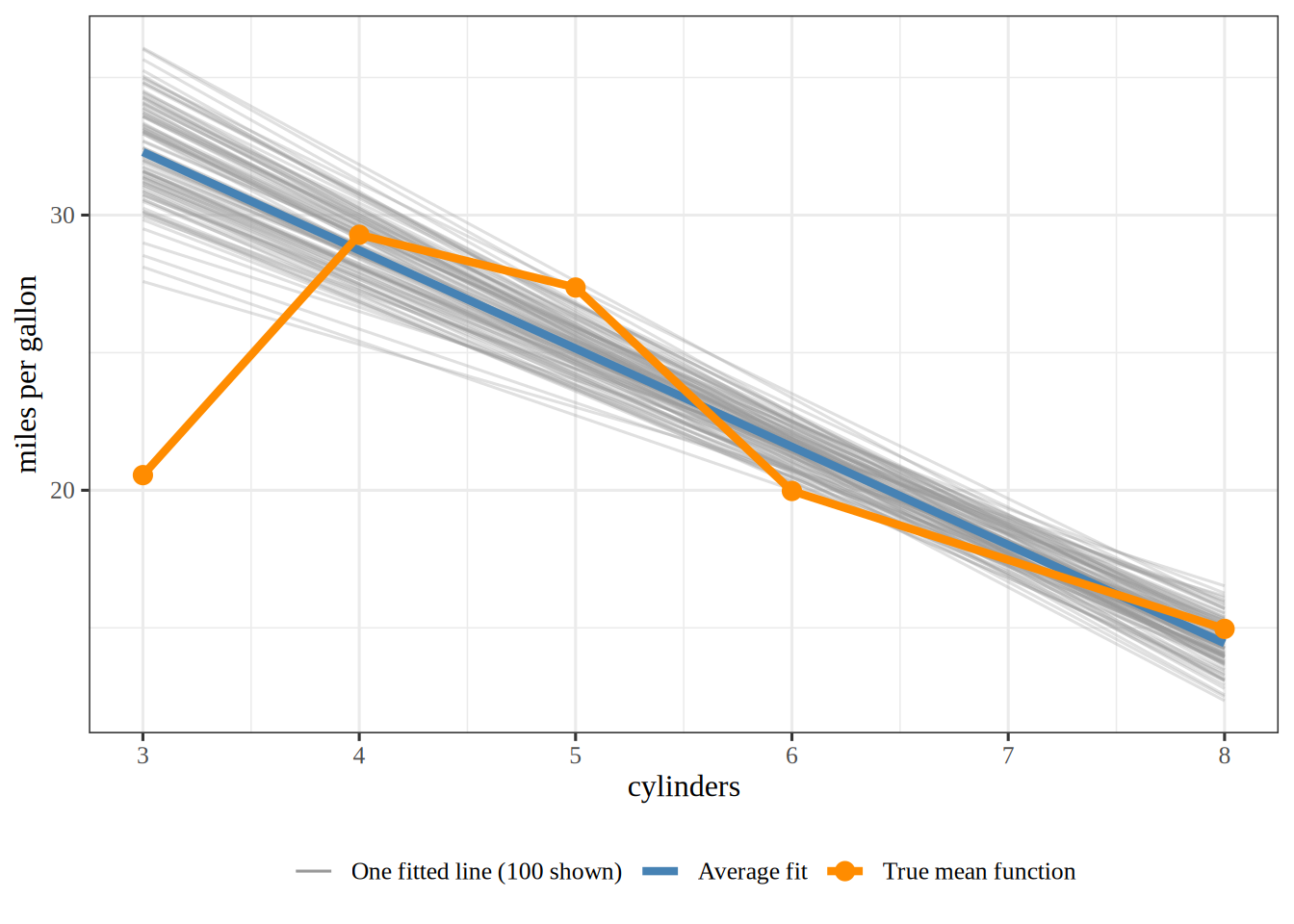
A plot of miles per gallon against cylinders, from 3 to 8. One hundred faint grey lines slope downward and fan out, most widely at 3 and 8 cylinders and most narrowly between 6 and 7 cylinders. A thick blue line, the average of all 2000 fitted lines, runs down through the middle of the grey lines. A thick orange line with points at 3, 4, 5, 6 and 8 cylinders, the mean mpg of the cars with that many cylinders, is not straight: it starts well below the blue line at 3 cylinders, rises above it at 4 and 5, and then follows it down to 8. A legend below the plot names the three: one fitted line, average fit, and true mean function.

Definition 3 (Bias of a prediction)

Definition 3 (Bias of a prediction) The bias of a prediction at \(\predvar\) is the expected prediction error of the prediction at \(\predvar\). The outcome in the prediction error is a new outcome \(\Outvar\) at \(\predvar\) in the noise model, so the error is \(\prederr = \devof{\predval}{\Outvar}\). The expectation is taken over training sets \(\trainset\) and over the noise in \(\Outvar\):

\[ \bias{\predval} \eqdef \Ep_{\trainset, \Outvar}\sb{\prederr} . \tag{3}\]

Example 5 (The bias of the cylinders line at four cylinders)

Example 5 (The bias of the cylinders line at four cylinders) Continue Example 4 with the same 2000 fitted lines. At \(x = 4\) cylinders, the value \(\truemeanf{4}\) of the true mean function in the noise model is the population mean mpg of the four-cylinder cars. Compute the bias (Equation 3) of the line:

Show code
import numpy as np

# mu(4) is the mean mpg of the four-cylinder cars.
f4_bv = mpg_af[cyl_af == 4].mean()

# Bias: the average fit minus the truth.
bias_bv = preds_af.mean() - f4_bv
print(np.round(bias_bv, 2))
-0.56
Show code
# mu(4) is the mean mpg of the four-cylinder cars.
f4_bv <- mean(auto_af$mpg[auto_af$cylinders == 4])

# Bias: the average fit minus the truth.
bias_bv <- mean(preds_af) - f4_bv
round(bias_bv, 2)
[1] -0.56

The average fit is 0.56 miles per gallon below the truth, so the bias is -0.56. The two tabs print the same number up to rounding.

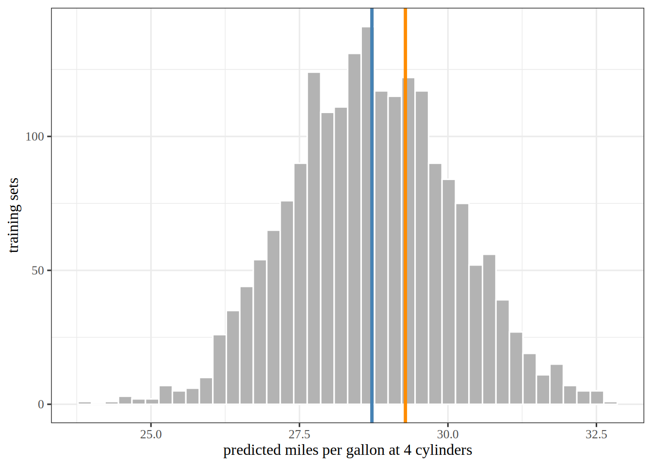
Figure 3 shows the 2000 predictions with the average fit and the true mean function at four cylinders. The histogram uses 40 bins; an even split of the 2000 predictions would put 50 in each bin. Forty bins are enough to show the shape of the histogram, which a few wide bins would flatten and a few hundred narrow bins would break into jagged spikes.

Show code
import matplotlib.pyplot as plt

fig, ax = plt.subplots(figsize=(6, 3.5), layout="constrained")
ax.hist(preds_af, bins=40, color="lightgrey", edgecolor="white");
ax.axvline(preds_af.mean(), color="steelblue", linewidth=2);
ax.axvline(f4_bv, color="darkorange", linewidth=2);
ax.set_xlabel("predicted miles per gallon at 4 cylinders");
ax.set_ylabel("training sets");
plt.show()
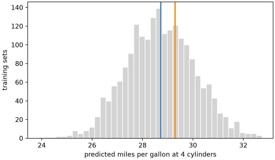
Figure 3: The 2000 predictions at four cylinders, with their average (the average fit, blue) and the true mean function at four cylinders (orange). The gap between the lines is the bias.
A histogram of 2000 predicted miles per gallon at four cylinders, roughly bell-shaped. A blue vertical line marks the mean of the predictions, near the centre of the histogram. An orange vertical line marks the mean mpg of the four-cylinder cars, a little to the right of the blue line, because the average fit is below the truth.
Show code
library(ggplot2)

ggplot(data.frame(prediction = preds_af), aes(prediction)) +
  geom_histogram(bins = 40, fill = "grey70", colour = "white") +
  geom_vline(xintercept = mean(preds_af), colour = "steelblue", linewidth = 1.2) +
  geom_vline(xintercept = f4_bv, colour = "darkorange", linewidth = 1.2) +
  labs(x = "predicted miles per gallon at 4 cylinders", y = "training sets")
A histogram of 2000 predicted miles per gallon at four cylinders, roughly bell-shaped. A blue vertical line marks the mean of the predictions, near the centre of the histogram. An orange vertical line marks the mean mpg of the four-cylinder cars, a little to the right of the blue line, because the average fit is below the truth.

Remark 5 (The sign of the bias)

Remark 5 (The sign of the bias). The bias is the expectation of a prediction error, so it is positive when the prediction \(\predval\) exceeds the new outcome \(\Outvar\) in expectation, and negative when the prediction falls short of the new outcome in expectation. The risk is the expected squared prediction error, so it is never negative. It adds the variance of the prediction and the residual variance to the square of the bias.

Definition 4 (Variance of a prediction)

Definition 4 (Variance of a prediction) The variance of a prediction at \(\predvar\) is the expected square of the deviation of the prediction at \(\predvar\) from its population mean over training sets \(\trainset\), which is the average fit \(\avgfitf{\predvar}\):

\[ \Var{\predval} = \Expfc{\trainset}{\sqf{\popdevf{\predval}}} , \quad \text{where } \popdevf{\predval} = \predval - \Epredval . \tag{4}\]

Example 6 (The variance of the cylinders line at four cylinders)

Example 6 (The variance of the cylinders line at four cylinders) Continue Example 5 with the same 2000 fitted models. Compute the variance (Equation 4) of their four-cylinder prediction:

Show code
# Variance: the mean squared deviation of a prediction from the average fit.
dev_var = preds_af - preds_af.mean()
var_bv = np.mean(dev_var ** 2)
print(np.round(var_bv, 2))
1.86
Show code
# Variance: the mean squared deviation of a prediction from the average fit.
avg_fit_var <- mean(preds_af)
dev_var <- preds_af - avg_fit_var
var_bv <- mean(dev_var^2)
round(var_bv, 2)
[1] 1.86

The variance is 1.86 squared miles per gallon: the sample mean, over the 2000 fitted models, of the squared deviation of a prediction from the average fit. The two tabs print the same number up to rounding.

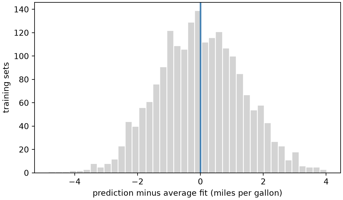
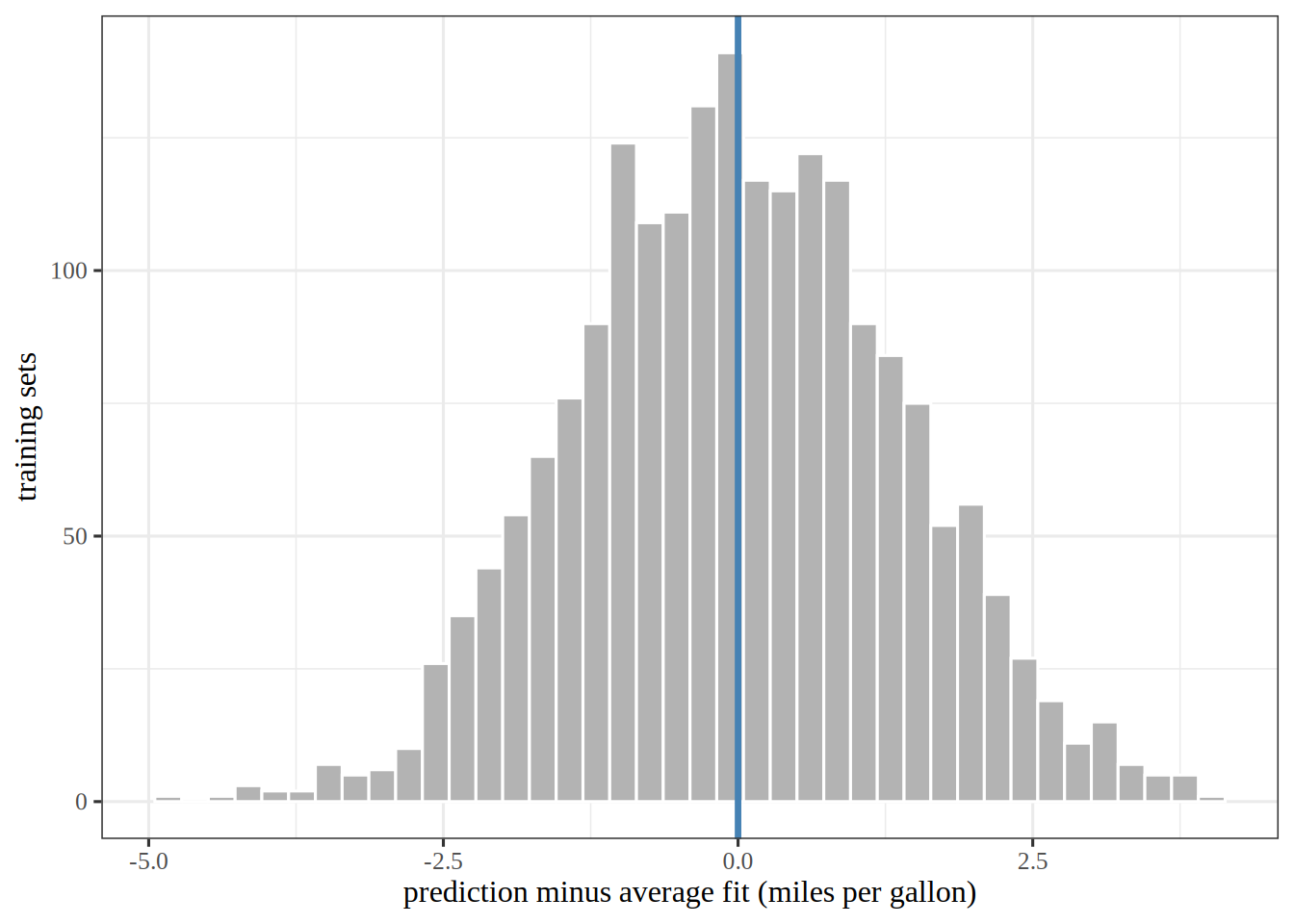
Figure 4 shows the 2000 deviations of the predictions from the average fit, in the same 40 bins as Figure 3 and for the same reason.

Show code
fig, ax = plt.subplots(figsize=(6, 3.5), layout="constrained")
ax.hist(dev_var, bins=40, color="lightgrey", edgecolor="white");
ax.axvline(0, color="steelblue", linewidth=2);
ax.set_xlabel("prediction minus average fit (miles per gallon)");
ax.set_ylabel("training sets");
plt.show()
Figure 4: The deviations of the 2000 predictions at four cylinders from their average fit. The variance is the mean of their squares, so a wider histogram means a larger variance.
A histogram of 2000 deviations, in miles per gallon, of the predictions at four cylinders from their average, roughly bell-shaped and centred on zero, where a blue vertical line marks zero.
Show code
dev_tbl_var <- tibble::tibble(deviation = dev_var)

dev_tbl_var |>
  ggplot() +
  aes(x = deviation) +
  geom_histogram(bins = 40, fill = "grey70", colour = "white") +
  geom_vline(xintercept = 0, colour = "steelblue", linewidth = 1.2) +
  labs(
    x = "prediction minus average fit (miles per gallon)",
    y = "training sets"
  )
A histogram of 2000 deviations, in miles per gallon, of the predictions at four cylinders from their average, roughly bell-shaped and centred on zero, where a blue vertical line marks zero.

Remark 6 (The variance of a fitted model’s prediction is the variance of a random variable)

Remark 6 (The variance of a fitted model’s prediction is the variance of a random variable). The prediction of the fitted model at \(\predvar\) is a random variable, because it depends on the training set \(\trainset\). The variance of that prediction is therefore the variance of that random variable.

Theorem 2 (The bias as the average fit minus the true mean function)

Theorem 2 (The bias as the average fit minus the true mean function) The bias of the prediction at \(\predvar\) equals the average fit minus the true mean function value:

\[ \bias{\predval} = \avgfitf{\predvar} - \truemeanf{\predvar} . \]

Proof

Proof. The mean of the new outcome \(\Outvar\) is the true mean function value \(\truemeanf{\predvar}\) because the noise has mean zero by the noise model.

\[ \begin{aligned} \bias{\predval} &= \Ep_{\trainset, \Outvar}\sb{\prederr} && \text{(definition of bias)} \\ &= \Ep_{\trainset, \Outvar}\sb{\devof{\predval}{\Outvar}} && \text{(definition of prediction error)} \\ &= \Epredval - \Ep_{\Outvar}\sb{\Outvar} && \text{(linearity of expectation)} \\ &= \Epredval - \truemeanf{\predvar} && \text{(the noise has mean zero)} \\ &= \avgfitf{\predvar} - \truemeanf{\predvar} && \text{(definition of the average fit)} . \end{aligned} \]

Example 7 (The bias as the average fit minus the true mean function at four cylinders)

Example 7 (The bias as the average fit minus the true mean function at four cylinders) Continue Example 5 with the same 2000 fitted lines. The bias is the expectation of the prediction error against a new outcome (Equation 3). The new outcome has mean \(\truemeanf{4}\), so the bias equals the average estimation error of the lines. Compute that average, and compare it with the average fit minus the truth:

# The bias from its definition: the mean error over the lines, taking the new outcome at its mean.
bias_def_baf = np.mean(preds_af - f4_bv)
# The bias from the theorem: the average fit minus the truth.
bias_thm_baf = preds_af.mean() - f4_bv
print(np.round([bias_def_baf, bias_thm_baf], 2))
[-0.56 -0.56]
# The bias from its definition: the mean error over the lines, taking the new outcome at its mean.
bias_def_baf <- mean(preds_af - f4_bv)
# The bias from the theorem: the average fit minus the truth.
bias_thm_baf <- mean(preds_af) - f4_bv
round(c(definition = bias_def_baf, theorem = bias_thm_baf), 2)
definition    theorem 
     -0.56      -0.56 

Both routes give -0.56 miles per gallon, as Theorem 2 says.

Theorem 3 (The variance equals the variance of the estimation error)

Theorem 3 (The variance equals the variance of the estimation error) The variance of the prediction of the fitted model at \(\predvar\) equals the variance of the estimation error of that prediction:

\[ \Var{\predval} = \Var{\erf{\predval}} . \]

Proof

Proof. The mean of the estimation error is the average fit minus the true mean function value, which is the bias by Theorem 2. Subtracting the bias from the error leaves the fit minus the average fit.

\[ \begin{aligned} \erf{\predval} - \bias{\predval} &= \paren{\predval - \truemeanf{\predvar}} - \paren{\Epredval - \truemeanf{\predvar}} && \text{(definition of estimation error; @thm-bias-average-fit)} \\ &= \predval - \truemeanf{\predvar} - \Epredval + \truemeanf{\predvar} && \text{(removing parentheses)} \\ &= \predval - \Epredval + \paren{\truemeanf{\predvar} - \truemeanf{\predvar}} && \text{(reordering)} \\ &= \predval - \Epredval + 0 && \text{(a number minus itself is zero)} \\ &= \predval - \Epredval && \text{(adding zero changes nothing)} . \end{aligned} \]

The error’s variance is its expected squared deviation from its own mean, and its mean is the bias. So the variance of the error is the expected square of the difference above. By Equation 4, the variance of the fit is the expected square of the same difference. So the two variances are equal.

Example 8 (The variance as the spread around the average fit at four cylinders)

Example 8 (The variance as the spread around the average fit at four cylinders) Continue Example 5 with the same 2000 fitted lines. Compute the variance of the lines (Equation 4), and compare it with the variance of their estimation error:

# The variance from the definition: the spread of the lines around the average fit.
var_def_vaf = np.mean((preds_af - preds_af.mean()) ** 2)
# The variance from the theorem: the spread of the estimation error around its mean, the bias.
err_vaf = preds_af - f4_bv
var_thm_vaf = np.mean((err_vaf - err_vaf.mean()) ** 2)
print(np.round([var_def_vaf, var_thm_vaf], 2))
[1.86 1.86]
# The variance from the definition: the spread of the lines around the average fit.
var_def_vaf <- mean((preds_af - mean(preds_af))^2)
# The variance from the theorem: the spread of the estimation error around its mean, the bias.
err_vaf <- preds_af - f4_bv
var_thm_vaf <- mean((err_vaf - mean(err_vaf))^2)
round(c(definition = var_def_vaf, theorem = var_thm_vaf), 2)
definition    theorem 
      1.86       1.86 

Both routes give 1.86 squared miles per gallon, as Theorem 3 says.

Five training sets of size five each get four fitted models, one for each polynomial degree from 1 to 4. Both tabs draw the training sets with the SyncRNG package [4] from the same seed, so they draw the same data, and add normal noise (standard deviation 0.13) to the true mean function:

Show code
import numpy as np
import matplotlib.pyplot as plt
from SyncRNG import SyncRNG


def truth_bv(x):
    return 0.55 - 0.9 * x + 0.6 * np.sin(6 * x)


x_bv = np.array([0.1, 0.3, 0.5, 0.7, 0.9])
grid_bv = np.linspace(0.05, 0.95, 100)

rng_bv = SyncRNG(seed=37)
# The first draws from a small seed are poorly mixed, so skip the first 100.
# With seed 37 the spread rises with the degree, and the line and quadratic have about the same bias; the text below the figure depends on that.
for _ in range(100):
    _ = rng_bv.rand()


def std_normal_bv():
    # One standard normal draw from two uniform draws (the Box-Muller transform).
    u1, u2 = rng_bv.rand(), rng_bv.rand()
    return np.sqrt(-2 * np.log(u1)) * np.cos(2 * np.pi * u2)


# Five training sets of five points.
samples_bv = [truth_bv(x_bv) + 0.13 * np.array([std_normal_bv() for _ in x_bv]) for _ in range(5)]
titles_bv = ["A line: high bias, low variance", "A quadratic", "A cubic", "A quartic: low bias, high variance"]

fig, axes = plt.subplots(2, 2, figsize=(6.5, 5), sharex=True, sharey=True, layout="constrained")
for degree, ax, title in zip(range(1, 5), axes.flat, titles_bv):
    # One fit per training set, evaluated on the grid.
    fits = np.array([np.polyval(np.polyfit(x_bv, y, degree), grid_bv) for y in samples_bv])
    for fit in fits:
        ax.plot(grid_bv, fit, color="#0072B2", linewidth=1);
    ax.plot(grid_bv, truth_bv(grid_bv), color="black", linestyle="--", linewidth=1.2);
    ax.set_title(title);
for ax in axes[1]:
    ax.set_xlabel("Feature, x");
for ax in axes[:, 0]:
    ax.set_ylabel("Response, y");
fig.legend(
    handles=[
        plt.Line2D([], [], color="#0072B2", label="One fit per training set"),
        plt.Line2D([], [], color="black", linestyle="--", label="The true mean function"),
    ],
    loc="outside lower center",
    ncol=2,
    frameon=False,
);
plt.show()
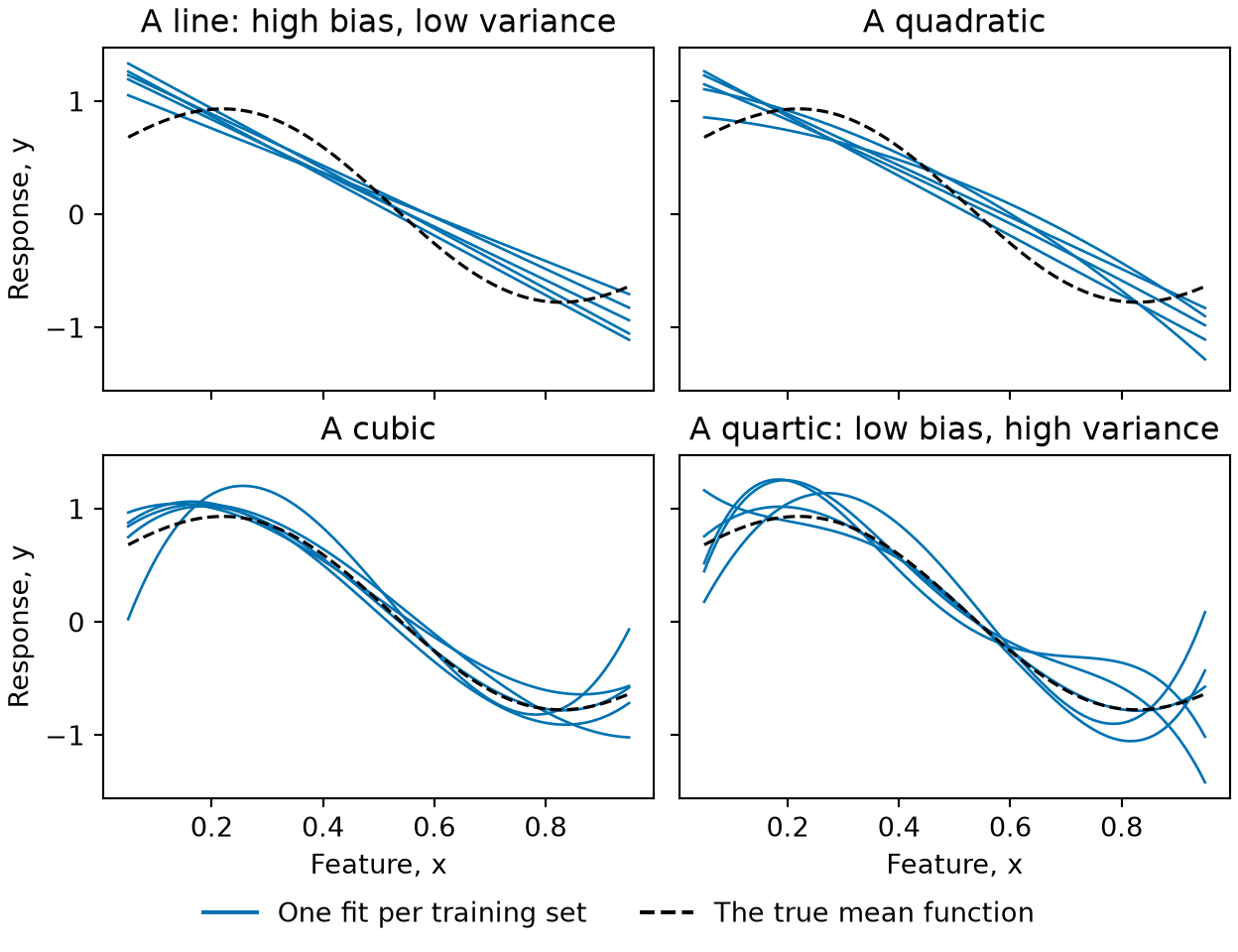
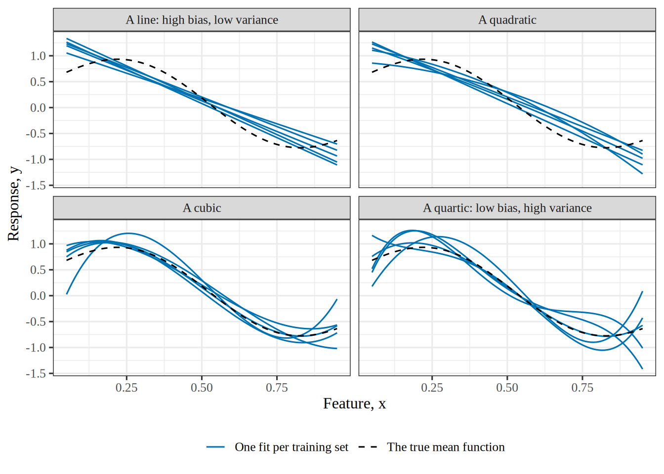
Figure 5: The same five training sets, fitted four times: by a line, a quadratic, a cubic and a quartic. The line and the quadratic lie close together and miss the true mean function (dashed) in the same places. The cubic fits follow it closely except near the ends of the range. The quartic fits, each passing through all five points of its training set, spread widely. Each curve is one training set’s fit, so the spread among the five is the variability itself.
Four panels in a two by two grid, each plotting y (from about -1.5 to 1.5) against x (from 0.05 to 0.95), with the true mean function as a dashed black curve that rises to a peak near x equal to 0.2, falls to a trough near 0.8, and five blue fitted curves, one per training set. Top left, a line: five nearly parallel straight lines slope downward and miss the true curve in the same way, too high at the left and too low near the right. Top right, a quadratic: five gently curved fits that also lie close together and miss the true curve in the same way. Bottom left, a cubic: five fits lie close to the true curve, except that one drops sharply at the left end and one rises at the right end. Bottom right, a quartic: five fits scatter widely around the true curve, swinging above and below it, most at the two ends.
Show code
library(ggplot2)
library(SyncRNG)

truth_bv <- function(x) 0.55 - 0.9 * x + 0.6 * sin(6 * x)
x_bv <- c(0.1, 0.3, 0.5, 0.7, 0.9)
grid_bv <- seq(0.05, 0.95, length.out = 100)

rng_bv <- SyncRNG(seed = 37)
# The first draws from a small seed are poorly mixed, so skip the first 100.
# With seed 37 the spread rises with the degree, and the line and quadratic have about the same bias; the text below the figure depends on that.
for (i in 1:100) rng_bv$rand()
# One standard normal draw from two uniform draws (the Box-Muller transform).
std_normal_bv <- function() {
  u <- c(rng_bv$rand(), rng_bv$rand())
  sqrt(-2 * log(u[1])) * cos(2 * pi * u[2])
}

# Five training sets of five points, each fitted by a polynomial of degree 1 to 4.
fits_bv <- do.call(rbind, lapply(1:5, function(set) {
  y <- truth_bv(x_bv) + 0.13 * replicate(5, std_normal_bv())
  do.call(rbind, lapply(1:4, function(degree) {
    fit <- lm(y ~ poly(x_bv, degree, raw = TRUE))
    data.frame(
      set = set,
      degree = factor(degree, levels = 1:4, labels = c("A line: high bias, low variance", "A quadratic", "A cubic", "A quartic: low bias, high variance")),
      x = grid_bv,
      fit = predict(fit, data.frame(x_bv = grid_bv))
    )
  }))
}))
truth_df_bv <- data.frame(x = grid_bv, fit = truth_bv(grid_bv))

# The spread of the five fits: their standard deviation at each x, averaged over the grid.
spread_bv <- sapply(split(fits_bv, fits_bv$degree), function(d) mean(tapply(d$fit, d$x, sd)))

ggplot(fits_bv, aes(x, fit)) +
  geom_line(aes(group = set, colour = "One fit per training set", linetype = "One fit per training set")) +
  geom_line(data = truth_df_bv, aes(colour = "The true mean function", linetype = "The true mean function")) +
  facet_wrap(~degree, nrow = 2) +
  scale_colour_manual(values = c("One fit per training set" = "#0072B2", "The true mean function" = "black")) +
  scale_linetype_manual(values = c("One fit per training set" = "solid", "The true mean function" = "dashed")) +
  labs(x = "Feature, x", y = "Response, y", colour = NULL, linetype = NULL)
Four panels in a two by two grid, each plotting y (from about -1.5 to 1.5) against x (from 0.05 to 0.95), with the true mean function as a dashed black curve that rises to a peak near x equal to 0.2, falls to a trough near 0.8, and five blue fitted curves, one per training set. Top left, a line: five nearly parallel straight lines slope downward and miss the true curve in the same way, too high at the left and too low near the right. Top right, a quadratic: five gently curved fits that also lie close together and miss the true curve in the same way. Bottom left, a cubic: five fits lie close to the true curve, except that one drops sharply at the left end and one rises at the right end. Bottom right, a quartic: five fits scatter widely around the true curve, swinging above and below it, most at the two ends.

Each quartic has five parameters, one for each input in its training set, so it fits that training set exactly and swings between its inputs, which is the variability the bottom-right panel shows. The line has two parameters and barely moves, and the quadratic and the cubic sit between the two. The spread of the five fits, averaged over the grid, is 0.08 for the line, 0.10 for the quadratic, 0.13 for the cubic and 0.18 for the quartic, so here it rises with every step in the degree.

Theorem 4 (Separating the noise from the expected error)

Theorem 4 (Separating the noise from the expected error) Choose an input value \(x\), and let the output variable \(Y = \truemeanf{x} + \noise\) as in the noise model, where \(\noise\) has mean \(0\) and variance \(\varpar\) and is independent of the training set \(\trainset\). Then the expected squared error at \(x\) is the noise variance \(\varpar\) plus the model’s own expected squared error:

\[ \Expfc{\trainset, \noise}{\sqf{Y - \predval}} = \varpar + \Expfc{\trainset}{\sqf{\truemeanf{x} - \predval}} . \tag{5}\]

Proof

Proof. This is the statistics notes’ theorem that the expected squared prediction error is the noise variance plus the expected squared estimation error, applied to the prediction \(\predval\) of the mean \(\truemeanf{x}\).

Example 9 (Separating the noise at four cylinders)

Example 9 (Separating the noise at four cylinders) Continue Example 4 with the same 2000 fitted lines, at \(x = 4\) cylinders, where \(\truemeanf{4}\) is the population mean mpg of the four-cylinder cars and the noise is how far a single car sits from that population mean. Compute the left side of Equation 5 directly, and then the noise variance plus the model’s own expected squared error:

y4_sn = mpg_af[cyl_af == 4]
f4_sn = y4_sn.mean()

# The left side: average the squared error over every line and every car.
left_sn = np.mean((y4_sn[None, :] - preds_af[:, None]) ** 2)
noise_sn = np.mean((y4_sn - f4_sn) ** 2)
model_sn = np.mean((f4_sn - preds_af) ** 2)
print(np.round([left_sn, noise_sn, model_sn, noise_sn + model_sn], 2))
[34.18 31.99  2.18 34.18]
y4_sn <- auto_af$mpg[auto_af$cylinders == 4]
f4_sn <- mean(y4_sn)

left_sn <- mean(outer(preds_af, y4_sn, function(h, y) (y - h)^2))
noise_sn <- mean((y4_sn - f4_sn)^2)
model_sn <- mean((f4_sn - preds_af)^2)
round(c(left = left_sn, noise = noise_sn, model = model_sn,
        sum = noise_sn + model_sn), 2)
 left noise model   sum 
34.18 31.99  2.18 34.18 

The expected squared error is 34.18, and the noise variance 31.99 plus the model’s own expected squared error 2.18 add to 34.18, as Theorem 4 says.

Theorem 5 (Separating the bias from the model’s own error)

Theorem 5 (Separating the bias from the model’s own error) Choose an input value \(x\), let \(\truemeanf{x}\) be the true mean function of the outcome variable given the input value \(x\) in the noise model, and let \(\avgfitf{x}\) be the average fit of Equation 2. Then the expected squared distance between the truth and the fitted model is the squared bias plus the variance:

\[ \Expfc{\trainset}{\sqf{\truemeanf{x} - \predval}} = \sqf{\truemeanf{x} - \Epredvalf{x}} + \Expfc{\trainset}{\sqf{\predval - \Epredvalf{x}}} . \tag{6}\]

Proof

Proof. The statistics notes work this as an exercise, separating the bias.

Example 10 (Separating the bias at four cylinders)

Example 10 (Separating the bias at four cylinders) Continue Example 4 with the same 2000 fitted lines, at \(x = 4\) cylinders, where \(\truemeanf{4}\) is the population mean mpg of the four-cylinder cars. Compute the left side of Equation 6 directly, and then the squared bias plus the variance:

f4_sb = mpg_af[cyl_af == 4].mean()

# The left side: average the squared distance from mu(4) over the lines.
left_sb = np.mean((f4_sb - preds_af) ** 2)
bias2_sb = (f4_sb - preds_af.mean()) ** 2
variance_sb = np.mean((preds_af - preds_af.mean()) ** 2)
print(np.round([left_sb, bias2_sb, variance_sb, bias2_sb + variance_sb], 2))
[2.18 0.32 1.86 2.18]
f4_sb <- mean(auto_af$mpg[auto_af$cylinders == 4])

left_sb <- mean((f4_sb - preds_af)^2)
bias2_sb <- (f4_sb - mean(preds_af))^2
variance_sb <- mean((preds_af - mean(preds_af))^2)
round(c(left = left_sb, bias2 = bias2_sb, variance = variance_sb,
        sum = bias2_sb + variance_sb), 2)
    left    bias2 variance      sum 
    2.18     0.32     1.86     2.18 

The model’s own expected squared error is 2.18, and the squared bias 0.32 plus the variance 1.86 add to 2.18, as Theorem 5 says.

Theorem 6 (Bias–variance decomposition)

Theorem 6 (Bias–variance decomposition) Choose an input value \(x\). By the noise model, a new output variable at \(x\) is \(Y = \truemeanf{x} + \noise\), where \(\truemeanf{x}\) is the value of the true mean function at \(x\) and \(\noise\) is the noise in this new output, whose population mean is \(0\) by Theorem 1. A learning algorithm fits a model to the training set \(\trainset\). Let \(\predval\) denote the model’s prediction for the input \(x\), which varies with \(\trainset\), and let \(\avgfitf{x}\) denote the average fit of that prediction. Assume that

  • \(\noise\) has variance \(\varpar < \infty\), and
  • \(\noise\) is independent of \(\trainset\), whose outputs contain their own separate noise draws.

Let \(\biassymf{\predval}\) denote \(\bias{\predval}\), the prediction’s bias, let \(\varsymf{\predval}\) denote \(\Var{\predval}\), its variance, and let \(\ESE{x}\) denote \(\Expfc{\trainset, \noise}{\sqf{Y - \predval}}\), the expected squared error of the prediction \(\predval\) of \(Y\).

Then \(\ESE{x}\) splits into three terms:

\[ \ESE{x} = \sqf{\biassymf{\predval}} + \varsymf{\predval} + \irrerr . \tag{7}\]

Proof

Proof. By Theorem 4 and Theorem 5, the expected squared error is the sum of the noise variance \(\irrerr\), \(\sqf{\truemeanf{x} - \Epredvalf{x}}\), and \(\Expfc{\trainset}{\sqf{\predval - \Epredvalf{x}}}\). The first is \(\irrerr\) itself. The second is the square of the bias of the prediction, because that bias is the average fit of the prediction minus the value of the true mean function of \(Y\) given \(X = x\), by Theorem 2. A square does not change when its base changes sign. The third is the variance of the prediction, by Equation 4.

Remark 7 (The decomposition holds for any algorithm)

Remark 7 (The decomposition holds for any algorithm). Equation 7 holds for any learning algorithm, and \(\noise\) need not be Gaussian. The statistics notes prove it as the bias, variance and noise decomposition of the expected squared prediction error.

Remark 8 (The error decomposition over training sets)

Remark 8 (The error decomposition over training sets). The reducible error and residual variance decomposition holds the training set \(\trainset\) fixed. Then the fitted model \(\fitmodf{\trainset}\) is fixed, and so is its prediction. That proposition writes the prediction at the input \(\vx\) as \(\ey\). This page writes the prediction at the input \(\predvar\) as \(\predval\). The prediction \(\predval\) depends on \(\trainset\), so it changes from one training set to the next. The expected squared error \(\ESE{\predvar}\) also takes the expectation over the noise and over training sets. There, the reducible error \(\sqf{\predval - \truemeanf{\predvar}}\) varies with \(\trainset\). So the expected squared error depends on the reducible error from every training set. Theorem 4 splits that expected squared error into two terms. The first term is the noise’s variance \(\varpar\). The second term is \(\Expfc{\trainset}{\sqf{\truemeanf{\predvar} - \predval}}\). By Theorem 5, that second term is \(\sqf{\biassymf{\predval}} + \varsymf{\predval}\), the squared bias plus the prediction’s variance.

Example 11 (Splitting the error of the cylinders line at four cylinders)

Example 11 (Splitting the error of the cylinders line at four cylinders) Continue Example 4 with the same 2000 fitted lines. The input is \(x = 4\) cylinders, and the output \(Y\) is the mpg of a four-cylinder car, so \(\truemeanf{4}\) is the population mean mpg of the four-cylinder cars and the noise is how far a single car sits from that population mean. Compute the three terms of Equation 7 and, separately, the expected squared error itself:

# Four-cylinder cars: their mean mpg is mu(4), and their spread is the noise.
y4_bv = mpg_af[cyl_af == 4]

bias2_bv = (y4_bv.mean() - preds_af.mean()) ** 2
variance_bv = np.mean((preds_af - preds_af.mean()) ** 2)
noise_bv = np.mean((y4_bv - y4_bv.mean()) ** 2)

# The left side: average the squared error over every line and every car.
error_bv = np.mean((y4_bv[None, :] - preds_af[:, None]) ** 2)
# Its Monte Carlo standard error: each line's mean squared error over the cars is one draw.
line_err_bv = np.mean((y4_bv[None, :] - preds_af[:, None]) ** 2, axis=1)
mc_se_bv = line_err_bv.std(ddof=1) / np.sqrt(len(line_err_bv))
print(np.round([bias2_bv, variance_bv, noise_bv, bias2_bv + variance_bv + noise_bv, error_bv], 2), round(mc_se_bv, 3))
[ 0.32  1.86 31.99 34.18 34.18] 0.067
y4_bv <- auto_af$mpg[auto_af$cylinders == 4]

bias2_bv <- (mean(y4_bv) - mean(preds_af))^2
variance_bv <- mean((preds_af - mean(preds_af))^2)
noise_bv <- mean((y4_bv - mean(y4_bv))^2)

# The left side: average the squared error over every line and every car.
err_mat_bv <- outer(preds_af, y4_bv, function(h, y) (y - h)^2)
error_bv <- mean(err_mat_bv)
# Its Monte Carlo standard error: each line's mean squared error over the cars is one draw.
line_err_bv <- rowMeans(err_mat_bv)
mc_se_bv <- sd(line_err_bv) / sqrt(length(line_err_bv))
c(round(c(bias2 = bias2_bv, variance = variance_bv, noise = noise_bv,
          sum = bias2_bv + variance_bv + noise_bv, error = error_bv), 2),
  mc_se = round(mc_se_bv, 3))
   bias2 variance    noise      sum    error    mc_se 
   0.320    1.860   31.990   34.180   34.180    0.067 

The three terms add to 34.18, which is the expected squared error 34.18 computed directly, as Theorem 6 says. That identity is exact for the 2000 lines and the cars used here. As an estimate of the expected squared error over all training sets, 34.18 has a 95% Monte Carlo confidence interval of 34.05 to 34.31. Most of it is the noise variance, 32.0: even a model with no bias and no variance would have that expected squared error on a four-cylinder car. The squared bias is only 0.32 and the variance 1.86. The decomposition holds for any learning algorithm, so the same arithmetic would split the error of a tree or a neural network.

Watch

Abu-Mostafa derives the same decomposition in his Caltech lecture on the bias–variance trade-off, from 16:43, and he reads bias and variance from learning curves, from 46:16 [5], Lecture 8.

Watch

Hastie and Tibshirani follow the bias–variance trade-off [6], video 2.3.

Watch

Weinberger explains the bias–variance decomposition [7], Lecture 19.

Watch

Starmer explains bias and variance [8] without the algebra.

Read

GeeksforGeeks explains the bias–variance trade-off [9].

1.1 Reading the decomposition

Exercise 3 (Read the three terms)

Exercise 3 (Read the three terms) Equation 7 splits the expected squared error at \(x\) into three terms. For each one, say what it measures, which panel of Figure 5 shows it large (if any), and whether a different learning algorithm or more data could make it smaller.

Solution 3. Only two of the three can be changed.

The first term, \(\sqf{\truemeanf{x} - \Epredvalf{x}}\), is the square of the bias (Definition 3) of \(\predval\) as an estimate of \(\truemeanf{x}\): how far the algorithm’s average fit is from the truth. It is a property of the family of models, not of any one fit. A straight line fitted to a curve has bias no amount of data will remove, because the average of many lines is still a line. That is the top-left panel of Figure 5, and the quadratic in the top-right panel behaves the same way: the five fits agree with each other and all differ from the truth in the same way. A different family can shrink it; more data cannot. A model whose error is mostly this term is said to underfit.

The second term, \(\Expfc{\trainset}{\sqf{\predval - \Epredvalf{x}}}\), is the variance (Definition 4) of \(\predval\): how far a single fit is from the average fit. It is a property of how strongly the algorithm reacts to its training data. The bottom-right panel of Figure 5 shows five quartics fitted to five samples from the same world, tracking the truth on average and differing strongly between the data points. More data or a less flexible family can shrink it. A model whose error is mostly this term is said to overfit.

The third term, \(\varpar\), is the noise in \(Y\) itself. No panel of Figure 5 shows it, because the figure plots only fitted curves and the truth, never the noisy data, and \(\varpar\) is the same for every family. It is not a fact about the model or the algorithm, and no method in these notes reduces it. It sets a lower limit: no model, however good, predicts better than \(\varpar\) on average. When a reported error is near that limit, little further improvement is possible; when a reported error is below it, something is wrong with how it was measured.

Definition 5 (Underfitting)

Definition 5 (Underfitting) A model is underfitting when the bias term of Equation 7 is large enough to dominate its error.

Definition 6 (Overfitting)

Definition 6 (Overfitting) A model is overfitting when the variance term of Equation 7 is large enough to dominate its error.

See overfitting in the statistics notes.

Show code
# HTML formats get an interactive plotly figure; the handout and other formats
# get the same two curves drawn with base R graphics.
set.seed(571)
truth <- function(x) sin(2 * pi * x)
noise_sd <- 0.3

# Fifteen training points and 500 fresh held-out points from the same curve.
n_train <- 15
n_held_out <- 500
x_train <- runif(n_train)
y_train <- truth(x_train) + rnorm(n_train, sd = noise_sd)
x_held <- runif(n_held_out)
y_held <- truth(x_held) + rnorm(n_held_out, sd = noise_sd)

# For each degree, fit by least squares on the training set and record the mean
# squared error on both sets, with the standard error of the held-out one.
degrees <- 1:10
errors <- sapply(degrees, function(d) {
  fit <- lm(y_train ~ poly(x_train, d))
  train_resid <- residuals(fit)
  held_pred <- predict(fit, newdata = data.frame(x_train = x_held))
  held_sq <- (y_held - held_pred)^2
  c(
    train = mean(train_resid^2),
    held = mean(held_sq),
    held_se = sd(held_sq) / sqrt(n_held_out)
  )
})
errors <- as.data.frame(t(errors))
errors$degree <- degrees

if (knitr::is_html_output()) {
  library(plotly)

  widget <- plot_ly() |>
    add_trace(
      data = errors, x = ~degree, y = ~train, type = "scatter",
      mode = "lines+markers", name = "training error",
      line = list(color = "#1f77b4"), marker = list(color = "#1f77b4")
    ) |>
    add_trace(
      data = errors, x = ~degree, y = ~held, type = "scatter",
      mode = "lines+markers", name = "held-out error (95% CI)",
      line = list(color = "#d95f02", dash = "dash"),
      marker = list(color = "#d95f02"),
      error_y = list(type = "data", array = ~ 1.96 * held_se, color = "#d95f02")
    ) |>
    layout(
      xaxis = list(title = "polynomial degree (flexibility)", dtick = 1),
      yaxis = list(title = "mean squared error", rangemode = "tozero"),
      legend = list(orientation = "h", y = -0.2),
      margin = list(t = 10)
    ) |>
    config(displaylogo = FALSE, responsive = TRUE)

  # The alt text: a plotly widget has none of its own.
  htmltools::div(
    role = "img",
    `aria-label` = paste(
      "Interactive plot of training error and held-out error against",
      "polynomial degree. Training error falls steadily; held-out error falls,",
      "bottoms out at a moderate degree and then rises."
    ),
    widget
  )
} else {
  # The legend goes below the plot, in a bottom margin made wide enough for it.
  op <- par(mar = c(8, 4, 1, 1))
  plot(
    errors$degree, errors$held, type = "b", col = "#d95f02", lty = 2, pch = 16,
    ylim = c(0, max(errors$held + 1.96 * errors$held_se)),
    xlab = "polynomial degree (flexibility)", ylab = "mean squared error"
  )
  arrows(
    errors$degree, errors$held - 1.96 * errors$held_se,
    errors$degree, errors$held + 1.96 * errors$held_se,
    angle = 90, code = 3, length = 0.03, col = "#d95f02"
  )
  lines(errors$degree, errors$train, type = "b", col = "#1f77b4", pch = 16)
  legend(
    "bottom", c("training error", "held-out error (95% CI)"),
    col = c("#1f77b4", "#d95f02"), lty = c(1, 2), pch = 16, bty = "n",
    horiz = TRUE, inset = c(0, -0.5), xpd = TRUE
  )
  par(op)
}
Figure 6: Training error and held-out error of polynomial fits of degree 1 to 10, fitted to 15 noisy points from a smooth curve. Training error only falls as the degree grows. Held-out error, estimated on 500 fresh points with a 95% confidence interval, falls while the fit is underfitting, then rises again as it overfits.

Read

GeeksforGeeks explains underfitting and overfitting [10].

Read

Domingos, a University of Washington professor, gives twelve lessons on generalization, overfitting and feature engineering in A Few Useful Things to Know About Machine Learning [11].

Exercise 4 (Predict weight from height)

Exercise 4 (Predict weight from height) Suppose we predict a person’s weight from their height. Could any model, given enough data, drive its expected squared error to zero?

Solution 4. No. The two are related, and yet no function of height alone will ever return weight exactly, because two people of the same height differ in ways that height does not record. That leftover spread is called the residual variance: the part of the output that the inputs do not determine.

Exercise 5 (Predict weight from height (part 2))

Exercise 5 (Predict weight from height (part 2)) Use the setup of Exercise 4.

If not, what would lower the minimum possible error?

Solution 5. Residual variance depends on the features and not on the model, so a better model leaves it unchanged. Record frame size too, and some of the spread can move out of the residual variance and into the part a model can learn. Averaged over the inputs, the residual variance does not rise when a feature is added, and it falls exactly when the feature changes the conditional mean of weight given height.

Definition 7 (Residual variance (residual noise variance, irreducible error))

Definition 7 (Residual variance (residual noise variance, irreducible error)) The residual variance (also called the residual noise variance or the irreducible error) at \(\predvar\) is the variance of the noise \(\noise\) in the noise model: the variance of the output \(\Outvar\) around its true mean function at \(\predvar\),

\[ \varpar \eqdef \Var{\noise} = \condVar{\Outvar}{\Predvar = \predvar} = \condE{\sqf{\Outvar - \truemeanf{\predvar}}}{\Predvar = \predvar} . \tag{8}\]

Remark 9 (What “irreducible” means)

Remark 9 (What “irreducible” means). The residual variance is the part of the expected squared error in Equation 7 that no choice of model or algorithm changes. It is a variance, a component of the expected loss. Textbooks call it the “irreducible error” [3, Sec. 2.1.1] [2], equation 7.9. That name can suggest that it is a prediction error, although it is a variance.

It is irreducible only given the inputs. It depends on which inputs the model observes. Averaged over new inputs, the residual variance is \(\E{\condVar{\Outvar}{\Predvar}}\). By the law of total variance, adding a feature never raises this average, and lowers it exactly when the feature changes the conditional mean of \(\Outvar\) given the other inputs. At a single \(\predvar\), the residual variance can rise or fall when a feature is added.

Remark 10 (Estimating the residual variance)

Remark 10 (Estimating the residual variance). The residual variance is a population quantity, which \(\evarpar\), computed from the residuals of a fitted model, estimates.

Remark 11 (Residual variance in the statistics notes)

Remark 11 (Residual variance in the statistics notes). The statistics notes define the same residual variance for the prediction at one covariate value \(x\). It is the \(\varpar\) term in their bias, variance and noise decomposition of the expected squared prediction error, which they prove step by step.

Show code
# HTML formats get an interactive plotly figure; the handout and other formats
# get the same points as a static SVG from tools/make_big_ideas_figures.py.
if (knitr::is_html_output()) {
  library(plotly)

  truth <- function(x) 0.5 + 0.3 * sin(5 * x)
  noise_sd <- 0.08

  # The points of the static figure. A fixed sine-based sequence stands in for
  # a random draw, so both versions show the same points; the noise is uniform
  # with standard deviation noise_sd.
  k <- 0:29
  wobble <- function(j) {
    v <- sin(j * 12.9898) * 43758.5453
    2 * (v - floor(v)) - 1
  }
  x_obs <- 0.02 + 0.96 * k / 29
  y_obs <- truth(x_obs) + noise_sd * sqrt(3) * wobble(211 + 5 * k)

  x_grid <- seq(0, 1, length.out = 200)

  widget <- plot_ly() |>
    add_trace(
      x = x_grid, y = truth(x_grid) + noise_sd, type = "scatter", mode = "lines",
      line = list(color = "rgba(0,0,0,0)"), hoverinfo = "skip", showlegend = FALSE
    ) |>
    add_trace(
      x = x_grid, y = truth(x_grid) - noise_sd, type = "scatter", mode = "lines",
      fill = "tonexty", fillcolor = "rgba(217,95,2,0.18)",
      line = list(color = "rgba(0,0,0,0)"), hoverinfo = "skip",
      name = "one noise standard deviation either side"
    ) |>
    add_trace(
      x = x_grid, y = truth(x_grid), type = "scatter", mode = "lines",
      name = "the true mean function μ", line = list(color = "#222222")
    ) |>
    add_trace(
      x = x_obs, y = y_obs, type = "scatter", mode = "markers",
      name = "observations", marker = list(color = "#1f77b4", size = 8)
    ) |>
    layout(
      xaxis = list(title = "Feature, x"), yaxis = list(title = "Response, y"),
      legend = list(orientation = "h", y = -0.2),
      margin = list(t = 10)
    ) |>
    config(displaylogo = FALSE, responsive = TRUE)

  # The alt text: a plotly widget has none of its own.
  htmltools::div(
    role = "img",
    `aria-label` = paste(
      "Interactive plot of a smooth true mean function with a band of one noise",
      "standard deviation on either side and thirty noisy points scattered",
      "around it."
    ),
    widget
  )
} else {
  knitr::include_graphics("../images/big-ideas/irreducible-error.svg")
}
Figure 7: Thirty points drawn from a true mean function plus noise. The band reaches one standard deviation of the noise above and below the true mean function, so its squared half-width is the residual variance \(\varpar\). Even a model that matches the true mean function exactly misses a typical point by about the half-width of the band, because the noise moves each point off the function. No model can predict the observed values more closely than the spread of the noise allows.

Exercise 6 (Error without noise)

Exercise 6 (Error without noise) Imagine a data-generating process with no noise at all: \(\Outvar = \truemeanf{\predvar}\) exactly, with \(\truemeanf{\predvar} = \sin(2.5\pi \predvar)\) on \(-1 \le \predvar \le 1\), a curve with two and a half full waves. A student fits polynomials of degree 1, 3, 5 and 7 by least squares to training sets of \(\nobs = 8\) points, and tests each fit on new points from the same curve.

The degree-7 polynomial passes through all eight training points. Which polynomial do you expect to predict best on new points?

Solution 6. Fit each degree to 200 training sets of \(\nobs = 8\) points, each an equally spaced grid on \([-1, 1]\) shifted a little further along from one set to the next, and split the error on 401 evenly spaced test points with Equation 7. The grids are fixed, not random, so the R and Python tabs compute the same numbers.

import numpy as np
import pandas as pd

# The target, with no noise: the test labels are exactly mu(x).
def f_nn(x):
    return np.sin(2.5 * np.pi * x)

n_nn, sets_nn = 8, 200
x_test_nn = np.linspace(-1, 1, 401)
rows_nn = []
for degree in (1, 3, 5, 7):
    fits, train_err = [], []
    for k in range(sets_nn):
        # Each training set is the same equally spaced grid, shifted a little.
        # Shifting by hand, rather than drawing random points,
        # makes the numbers identical in the R tab.
        x = -1 + 2 / n_nn * (np.arange(n_nn) + (k + 0.5) / sets_nn)
        coef = np.linalg.lstsq(np.vander(x, degree + 1), f_nn(x), rcond=None)[0]
        fits.append(np.vander(x_test_nn, degree + 1) @ coef)
        train_err.append(np.mean((np.vander(x, degree + 1) @ coef - f_nn(x)) ** 2))
    fits = np.array(fits)
    avg_fit = fits.mean(axis=0)
    # The three terms of the decomposition. Noise is zero, so there are only two.
    bias2 = np.mean((avg_fit - f_nn(x_test_nn)) ** 2)
    variance = np.mean(fits.var(axis=0))
    rows_nn.append((degree, np.mean(train_err), bias2, variance, bias2 + variance))
print(pd.DataFrame(rows_nn, columns=["degree", "train", "bias2", "variance", "error"]).round(3))
   degree  train  bias2  variance  error
0       1  0.494  0.500     0.006  0.506
1       3  0.430  0.441     0.016  0.457
2       5  0.102  0.743     0.389  1.132
3       7  0.000  1.465     0.862  2.327
# The target, with no noise: the test labels are exactly mu(x).
f_nn <- function(x) sin(2.5 * pi * x)

n_nn <- 8
sets_nn <- 200
x_test_nn <- seq(-1, 1, length.out = 401)
nn_results <- do.call(rbind, lapply(c(1, 3, 5, 7), function(degree) {
  # Each training set is the same equally spaced grid, shifted a little.
  # Shifting by hand, rather than drawing random points,
  # makes the numbers identical in the Python tab.
  fits <- sapply(seq_len(sets_nn) - 1, function(k) {
    x <- -1 + 2 / n_nn * (seq_len(n_nn) - 1 + (k + 0.5) / sets_nn)
    design <- outer(x, 0:degree, "^")
    coef <- qr.solve(design, f_nn(x))
    c(test = drop(outer(x_test_nn, 0:degree, "^") %*% coef),
      train = mean((design %*% coef - f_nn(x))^2))
  })
  test_fits <- fits[seq_along(x_test_nn), ]
  avg_fit <- rowMeans(test_fits)
  # The three terms of the decomposition. Noise is zero, so there are only two.
  bias2 <- mean((avg_fit - f_nn(x_test_nn))^2)
  variance <- mean(apply(test_fits, 1, var) * (sets_nn - 1) / sets_nn)
  data.frame(degree = degree, train = mean(fits["train", ]),
             bias2 = bias2, variance = variance, error = bias2 + variance)
}))
round(nn_results, 3)

The cubic has the lowest error, 0.46, and the line is close behind at 0.51. The septic, which fits all eight training points exactly (training error 0.00), has the highest, 2.33.

Expect the low degrees to win, though the degree-7 fit has the best training error. With eight points, the degree-7 fit has no freedom left over, so each shifted training set bends it differently (variance 0.86).

Exercise 7 (Error without noise (part 2))

Exercise 7 (Error without noise (part 2)) Use the setup of Exercise 6.

The residual variance \(\varpar\) of Definition 7 is zero here. Where, then, does the error of the best polynomial come from?

Solution 7. The error comes from the model, not from the world. A line, or even a cubic, cannot follow two and a half waves, so every fit misses the curve in the same way (squared bias 0.50 for the line). A flexible polynomial passes through the curve at the training points and still goes wrong between them, because eight points are too few to pin it down there. Either way, the part of \(\truemean\) the model cannot learn from this much data acts on the fit like noise in the labels, which the definition of deterministic noise below makes precise.

Figure 8 draws the fits behind the table above: the curves each training set produces, their average, and the error by degree.

Figure 8: Fits to a noiseless curve, \(\truemean\), from 200 shifted grids of 8 points. Top: for each polynomial degree, 40 of the 200 fitted curves (grey), their average (colour) and one training set (dots). The line and the cubic miss the curve in the same way every time; the degree-7 polynomial passes through every training set and still swings wildly between the points. Bottom: training and test root mean squared error (RMSE) by degree, with the bars spanning the middle 95% of the 200 training sets.

Definition 8 (Best member of a model family)

Definition 8 (Best member of a model family) The best member \(\bestmod\) of a mean-function model family \(\modelfam\) for a target function \(\truemean\) is the member \(\modmem\) of \(\modelfam\) with the smallest mean squared difference from \(\truemean\), \(\E{\paren{\truemeanf{\Predvar} - \modmemf{\Predvar}}^2}\), where the random predictor \(\Predvar\) is a draw of the predictor \(\predvar\) from the population.

Example 12 (The best line for a curved target)

Example 12 (The best line for a curved target) Let the target \(\truemean\) be a sine curve, and let \(\modelfam\) be the family of straight lines. No line follows a sine curve, but some lines are closer to it than others, averaging the squared gap over the population of \(\predvar\). The closest line is the best member \(\bestmod\). A line fitted to a training set is a different object, because it depends on the data and so usually differs from \(\bestmod\).

Definition 9 (Deterministic noise)

Definition 9 (Deterministic noise) The deterministic noise of a mean-function model family \(\modelfam\) at \(\predvar\) is the part of \(\truemeanf{\predvar}\) that the family cannot express: \(\truemeanf{\predvar} - \bestmodf{\predvar}\), where \(\bestmod\) is the best member of \(\modelfam\) (Definition 8).

Remark 12 (Deterministic versus stochastic noise)

Remark 12 (Deterministic versus stochastic noise). Deterministic noise differs from the noise \(\noise\) in the labels of the noise model, which we call stochastic noise when we need to tell the two apart, in two ways:

  • Deterministic noise depends on the family: a richer family leaves less of \(\truemean\) unexpressed.
  • Deterministic noise is fixed for a given \(\predvar\): drawing a new training set does not change it.

Watch

Abu-Mostafa separates stochastic from deterministic noise in his Caltech lecture on overfitting [5], Lecture 11; the same chapter of his book, Abu-Mostafa et al. [1, Ch. 4], gives the written treatment.

Exercise 8 (Why the ranking was wrong)

Exercise 8 (Why the ranking was wrong) The table of empirical risk by degree ranked the fitted polynomials by their training error, and the quartic came first. Which of the three terms of Equation 7 does training-set error measure?

Solution 8. None of them. Training-set error is an optimistic estimate of the expected error on the left-hand side of Equation 7.

Exercise 9 (Why the ranking was wrong (part 2))

Exercise 9 (Why the ranking was wrong (part 2)) Use the setup of Exercise 8.

Why does the ranking by training-set error favor the most flexible family?

Solution 9. Training error grows more optimistic with flexibility, because a more flexible model can fit the particular noise in its training set. So the quantity the table of empirical risk by degree ranks by improves for exactly the reason the variance term worsens.

Remark 13 (The bias-variance tradeoff)

Remark 13 (The bias-variance tradeoff). Across the families of Figure 5, more flexibility gives lower bias but higher variance: the line and the quadratic miss the truth in the same way every time, the cubic follows it closely, and the quartics swing apart from one another. Because of that trade, model selection needs careful study and is not a routine step. For the crime data, ranking the polynomials by training error put the quartic first because it is the most flexible, not because it predicts best (Exercise 8), so choosing the degree takes more than comparing the training errors.

Exercise 10 (Changes along the tradeoff)

Exercise 10 (Changes along the tradeoff) List changes you could make to the data or the model that shrink one of the two correctable terms of Equation 7. For each, say in which direction it changes the bias term and in which direction it changes the variance term.

Solution 10. Both correctable terms change in opposite directions as flexibility changes, so the usual changes are:

  • more data, which shrinks variance and leaves bias alone;
  • a smaller model family, which lowers variance and raises bias;
  • a larger model family, which does the reverse;
  • keeping the family but penalizing the size of the fitted parameters, which deliberately accepts a little bias in exchange for a larger reduction in variance.

Exercise 11 (Why would anyone choose the less flexible model?)

Exercise 11 (Why would anyone choose the less flexible model?) A straight line can only tilt; a high-degree polynomial can bend almost any way. Give two reasons the city in the crime example might still prefer the straight line: one that applies if it wants to explain how crime varies with income, and one that applies even if it only wants to predict.

Solution 11.

  • To explain, the line is readable. Its slope says how much the predicted crime rate changes per unit of income, and its sign says in which direction. The quartic of the exercise “Which model was actually better?” has no single number like that: each of its five coefficients multiplies a different power of income, so none of them alone says how crime changes with income, even when the curve predicts well. James et al. [12, Sec. 2.1.3] calls this the trade-off between flexibility and interpretability.

  • To predict, the line may simply be more accurate. With five neighborhoods, a flexible fit spends its freedom chasing those five points. Figure 5 shows what that costs: flexible fits to different samples from the same population disagree wildly with each other, so a prediction for a sixth neighborhood depends on which five happened to be sampled. That is the variance term of Equation 7, so the quartic’s perfect fit to its training set in the exercise “Which model was actually better?” was no evidence that it predicts well. James et al. [12, Sec. 2.1.3] makes the same point: even when only prediction matters, a less flexible method often predicts more accurately, because a very flexible one can overfit (Definition 6).

Neither reason makes the line the right choice by default. If the true relationship bends, the line’s bias does not shrink with more data.

Definition 10 (Regularization)

Definition 10 (Regularization) Regularization is fitting a model by minimizing its empirical risk plus a penalty on the size of its parameters [13]. With a penalty function \(\operatorname{pen}(\param) \ge 0\) and a penalty weight \(\regpar \ge 0\), regularization minimizes the objective plus the weighted penalty,

\[ \objfnf{\param} + \regpar \operatorname{pen}(\param) . \tag{9}\]

Example 13 (Regularizing the crime-data quartic)

Example 13 (Regularizing the crime-data quartic) For the polynomial fits to the crime data in the table of empirical risk by degree, a penalty on the coefficients makes a large coefficient on \(x^4\) costly, so the fitted quartic moves closer to a flatter curve that bends to fit each of the five neighborhoods less closely.

Definition 11 (Penalty weight (regularization strength))

Definition 11 (Penalty weight (regularization strength)) A penalty weight \(\lambda \ge 0\), also called the regularization strength, is the number that scales a penalty \(\operatorname{pen}(\param) \ge 0\), a nonnegative measure of the size of a model’s parameters, when the penalty is added to the training objective in regularization. The value \(\lambda = 0\) leaves the objective unchanged, and a larger \(\lambda\) penalizes large parameters more heavily.

Show code
# HTML formats get an interactive plotly figure (click the legend to hide a
# curve); the handout and other formats get the same curves with base R
# graphics.
set.seed(571)
truth <- function(x) sin(2 * pi * x)
n_points <- 12
x_obs <- sort(runif(n_points))
y_obs <- truth(x_obs) + rnorm(n_points, sd = 0.3)

# A degree-9 polynomial basis in a rescaled x, so that the powers are on
# comparable scales: a column of ones, then x^1 through x^9.
degree <- 9
basis <- function(x) cbind(1, outer(2 * x - 1, 1:degree, "^"))

# Penalized least squares: minimize the squared error plus the penalty weight
# times the sum of squared coefficients, leaving the intercept unpenalized. The
# tiny extra diagonal term only keeps the unpenalized fit numerically solvable.
penalized_fit <- function(penalty) {
  design <- basis(x_obs)
  penalty_matrix <- diag(c(0, rep(1, degree)))
  solve(
    crossprod(design) + penalty * penalty_matrix + 1e-10 * diag(degree + 1),
    crossprod(design, y_obs)
  )
}

penalties <- c(0, 0.001, 0.1)
labels <- c("no penalty", "penalty weight 0.001", "penalty weight 0.1")
colors <- c("#d95f02", "#1b9e77", "#7570b3")
x_grid <- seq(0, 1, length.out = 200)
curves <- lapply(
  penalties,
  function(p) drop(basis(x_grid) %*% penalized_fit(p))
)

if (knitr::is_html_output()) {
  library(plotly)

  widget <- plot_ly() |>
    add_trace(
      x = x_grid, y = truth(x_grid), type = "scatter", mode = "lines",
      name = "the true curve", line = list(color = "#999999", dash = "dot")
    )
  for (i in seq_along(penalties)) {
    widget <- widget |>
      add_trace(
        x = x_grid, y = curves[[i]], type = "scatter", mode = "lines",
        name = labels[i], line = list(color = colors[i])
      )
  }
  widget <- widget |>
    add_trace(
      x = x_obs, y = y_obs, type = "scatter", mode = "markers",
      name = "observations", marker = list(color = "#1f77b4", size = 8)
    ) |>
    layout(
      xaxis = list(title = "Feature, x"),
      yaxis = list(title = "Response, y", range = c(-2, 2)),
      legend = list(orientation = "h", y = -0.2),
      margin = list(t = 10)
    ) |>
    config(displaylogo = FALSE, responsive = TRUE)

  # The alt text: a plotly widget has none of its own.
  htmltools::div(
    role = "img",
    `aria-label` = paste(
      "Interactive plot of twelve noisy points and four curves: the",
      "true curve, an unpenalized degree-9 polynomial that swings wildly",
      "between the points, and two penalized fits that are progressively",
      "smoother."
    ),
    widget
  )
} else {
  # The legend goes below the plot, in a bottom margin made wide enough for it.
  op <- par(mar = c(9, 4, 1, 1))
  plot(
    x_obs, y_obs, pch = 16, col = "#1f77b4", ylim = c(-2, 2),
    xlab = "Feature, x", ylab = "Response, y"
  )
  lines(x_grid, truth(x_grid), col = "#999999", lty = 3)
  for (i in seq_along(penalties)) lines(x_grid, curves[[i]], col = colors[i])
  legend(
    "bottom", c("the true curve", labels, "observations"), ncol = 2, cex = 0.7,
    col = c("#999999", colors, "#1f77b4"), lty = c(3, 1, 1, 1, NA),
    pch = c(NA, NA, NA, NA, 16), bty = "n", inset = c(0, -0.62), xpd = TRUE
  )
  par(op)
}
Figure 9: A degree-9 polynomial fitted to 12 noisy points from a smooth curve, with a penalty on the size of its coefficients. With no penalty, the fit passes close to every point and swings wildly between them. A larger penalty weight pulls the fit toward a smoother curve that follows the points less closely.

Read

GeeksforGeeks explains regularization [14].

Exercise 12 (Read the response to a change, name the term)

Exercise 12 (Read the response to a change, name the term) Each of the following describes what happened when you changed one thing about a model and scored it honestly again. For each, say which term of Equation 7 the response points at, and what you would try next.

Strengthening the regularization penalty raises training error a little and lowers held-out error.

Solution 12. Variance. A stronger penalty limits how closely the fitted model can adapt to the peculiarities of one training set, so it shrinks \(\Expfc{\trainset}{\sqf{\predval - \Epredvalf{\predvar}}}\) at the cost of a little bias. Held-out error fell, so the variance removed outweighed the bias added. Keep raising the penalty while held-out error keeps falling, and stop where it starts to rise.

Exercise 13 (Read the response to a change, name the term (part 2))

Exercise 13 (Read the response to a change, name the term (part 2)) Use the setup of Exercise 12.

Doubling the training set does not change held-out error, but switching to a more flexible model family lowers training and held-out error together.

Solution 13. Bias. More data cuts variance, because each fit then depends less on the peculiarities of one training set, but it does not move the average fit \(\avgfit\) toward the truth. A held-out error that does not move with twice the data is therefore not mainly coming from variance. A more flexible family can place \(\avgfit\) closer to the truth, so both errors fell when you switched. Keep adding flexibility, or better features, while held-out error keeps falling.

Exercise 14 (Read the response to a change, name the term (part 3))

Exercise 14 (Read the response to a change, name the term (part 3)) Use the setup of Exercise 12.

Training error and held-out error are both small and roughly equal, and collecting ten times as much data changes neither.

Solution 14. Residual variance, most likely. Both errors agree, so variance is small; both are small, so bias is small; and more data moving neither says the remaining error is not a property of the model at all. There is nothing left to try on the modeling side. The remaining options are outside the model: measure the inputs more precisely, or find a feature that carries information the current ones do not.

Exercise 15 (A perfect algorithm)

Exercise 15 (A perfect algorithm) Suppose an algorithm has zero bias and zero variance at every \(x\), so every training set gives it the same fit, and that fit is \(f\). Can the risk of its fitted model still be nonzero? Use Equation 7 to say why or why not, and say what each of the two zeros means in words.

Solution 15. Yes: the expected squared error at \(x\) is then \(\varpar\), because the other two terms of Equation 7 are zero. The risk is nonzero whenever the noise is.

Zero variance means the algorithm returns the same fitted model on every training set, so it ignores its data. Zero bias means that model is the truth, \(\Epredvalf{x} = \truemeanf{x}\). Both zeros together describe an algorithm with nothing left to learn, and even that algorithm cannot predict \(Y\) more closely than the noise allows.

Remark 14 (Bias and variance for a classifier)

Remark 14 (Bias and variance for a classifier). The decomposition of Theorem 6 is for squared error, and it does not carry over to a classifier’s zero-one loss as an exact sum. For a classifier the words are an analogy. The Bayes error plays the part of the residual variance: no classifier using the same features does better. Under zero-one loss, bias and variance combine multiplicatively rather than additively [15, Sec. 6]. A classifier’s error at \(x\) depends on the bias only through the boundary bias, which records how far the average fit lies from the decision threshold and on which side. A fit that is very biased but on the correct side of the threshold is not penalized for that bias. In that case, reducing variance alone moves the error toward the Bayes error. Friedman puts it as “variance tends to dominate bias for classification” [15, Sec. 7], p. 63. He also shows the opposite case: where the average fit is on the wrong side of the threshold, reducing variance makes the error worse [15, Sec. 7], p. 62.

In Figure 10, raise the degree and watch the fits spread out; then choose more points per training set and see which term responds.

Figure 10: The decomposition of Equation 7, estimated by simulation. Polynomials of the chosen degree are fitted to 200 training sets drawn from a simulated world, each at the same evenly spaced inputs with fresh noise. The world is simulated, unlike the Auto data of the training and held-out error figure, because separating bias, variance and noise needs a true mean function that is known: here it is the dashed curve, with Gaussian noise of standard deviation 0.1. The left panel draws 20 of the fits and the average of all 200, with a pale band holding the middle 95% of the 200 fits at each \(x\), and the right panel averages each term over \(x\). The right panel has no interval band: each curve is a simulation average with a Monte Carlo error that is small beside the gaps between the terms, but it is not drawn, and redrawing the training sets shows how much the curves move.

Reading

Watch

Andrew Ng’s short lectures for DeepLearning.AI cover the same ideas for neural networks: how to read underfitting and overfitting as bias and variance [16], and a basic recipe for deciding what to change next [17].

Dependency graph

Open the block to see every definition and result of this page, with prerequisites at the top. Click a box to jump to it.

References

[1]
Y. S. Abu-Mostafa, M. Magdon-Ismail, and H.-T. Lin, Learning from data: A short course. AMLBook, 2012. Available: https://amlbook.com/
[2]
T. Hastie, R. Tibshirani, and J. Friedman, The elements of statistical learning: Data mining, inference, and prediction, 2nd ed. Springer, 2009. Available: https://hastie.su.domains/ElemStatLearn/
[3]
G. James, D. Witten, T. Hastie, and R. Tibshirani, An introduction to statistical learning with applications in R, 2nd ed. Springer, 2021. Available: https://www.statlearning.com/
[4]
G. van den Burg, SyncRNG: A synchronized Tausworthe RNG for R and Python. 2024. doi: 10.32614/CRAN.package.SyncRNG.
[5]
Y. S. Abu-Mostafa, “Learning from data: CS 156 lectures.” Caltech, lecture videos on YouTube, 2012. Available: https://www.youtube.com/playlist?list=PLD63A284B7615313A
[6]
T. Hastie, R. Tibshirani, and J. Taylor, “Statistical learning with python.” Stanford Online, lecture videos on YouTube, 2023. Available: https://www.youtube.com/playlist?list=PLoROMvodv4rPP6braWoRt5UCXYZ71GZIQ
[7]
K. Weinberger, “CS4780: Machine learning for intelligent systems, spring 2017.” Cornell University, lecture videos on YouTube, 2017. Available: https://www.youtube.com/playlist?list=PLl8OlHZGYOQ7bkVbuRthEsaLr7bONzbXS
[8]
J. Starmer, “Machine learning fundamentals: Bias and variance.” StatQuest, video on YouTube, 2018. Available: https://www.youtube.com/watch?v=EuBBz3bI-aA
[9]
GeeksforGeeks, “Bias-variance trade off - machine learning.” GeeksforGeeks, tutorial article, 2026. Available: https://www.geeksforgeeks.org/machine-learning/ml-bias-variance-trade-off/
[10]
GeeksforGeeks, “Underfitting and overfitting in ML.” GeeksforGeeks, tutorial article, 2025. Available: https://www.geeksforgeeks.org/machine-learning/underfitting-and-overfitting-in-machine-learning/
[11]
P. Domingos, “A few useful things to know about machine learning,” Communications of the ACM, vol. 55, no. 10, pp. 78–87, 2012, doi: 10.1145/2347736.2347755.
[12]
G. James, D. Witten, T. Hastie, R. Tibshirani, and J. Taylor, An introduction to statistical learning: With applications in Python. Springer, 2023. doi: 10.1007/978-3-031-38747-0.
[13]
Wikipedia contributors, “Regularization (mathematics) — Wikipedia, the free encyclopedia.” 2026. Available: https://en.wikipedia.org/wiki/Regularization_(mathematics)
[14]
GeeksforGeeks, “Regularization in machine learning.” GeeksforGeeks, tutorial article, 2026. Available: https://www.geeksforgeeks.org/machine-learning/regularization-in-machine-learning/
[15]
J. H. Friedman, “On bias, variance, 0/1—loss, and the curse-of-dimensionality,” Data Mining and Knowledge Discovery, vol. 1, no. 1, pp. 55–77, 1997, doi: 10.1023/A:1009778005914.
[16]
A. Ng, “Bias/variance.” DeepLearning.AI, Deep Learning Specialization, Course 2; video on YouTube, 2017. Available: https://www.youtube.com/watch?v=SjQyLhQIXSM
[17]
A. Ng, “Basic recipe for machine learning.” DeepLearning.AI, Deep Learning Specialization, Course 2; video on YouTube, 2017. Available: https://www.youtube.com/watch?v=C1N_PDHuJ6Q