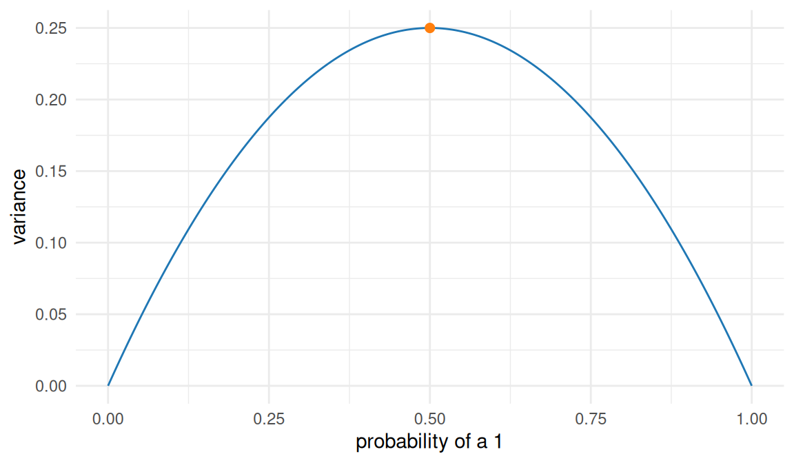
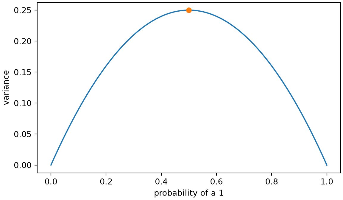
import numpy as np
import matplotlib.pyplot as plt
prob = np.linspace(0, 1, 201)
variance = prob * (1 - prob)
fig, ax = plt.subplots(figsize=(6, 3.5), layout="constrained")
ax.plot(prob, variance, color="#1f77b4")
ax.plot(0.5, 0.5 * (1 - 0.5), "o", color="#ff7f0e")
ax.set_xlabel("probability of a 1")
ax.set_ylabel("variance")
plt.show()Variance and covariance
1 Deviation, error, and noise
Definition 1 (Deviation) A deviation is the difference between a value and a reference value. For any quantity \(z\) and reference value \(r\), the deviation of \(z\) from \(r\) is:
\[z - r\]
Remark. In probability and statistics, “deviation” usually means deviation from a population mean.
Example 1 (Deviation from a reference weight) A newborn weighing 3,200 g deviates from a reference weight of 3,500 g by \(3200 - 3500 = -300\) g.
Definition 2 (Deviation from a population or subpopulation mean (error, noise term)) The deviation from the mean of a random variable \(Y\) is its deviation from its expectation, also called its error or noise term:
\[\mathbb{d}(Y) \stackrel{\text{def}}{=}Y - {\mathbb{E}\mathopen{}\left[Y\right]\mathclose{}}\]
For a realized observation \(y\):
\[\mathbb{d}(y) \stackrel{\text{def}}{=}y - {\mathbb{E}\mathopen{}\left[Y\right]\mathclose{}}\]
Remark. Other sources often call this quantity an error or noise term [1]. In regression settings, the reference mean is often conditional on covariates: \(\mathbb{d}(y_i) \stackrel{\text{def}}{=}y_i - {\mathbb{E}\mathopen{}\left[Y_i \mid X_i = x_i\right]\mathclose{}}\).
These notes prefer “deviation” for the quantity just defined. The Morrison Lab’s regression notes use “residual” (defined in their Linear regression chapter) for deviations from fitted values, write \(\mathbb{d}(\cdot)\) for these model/data deviations, and reserve \({\varepsilon\mathopen{}\left(\cdot\right)\mathclose{}}\) for estimator-to-estimand deviations (see Estimation).
See:
Example 2 (Deviation of a die roll from its mean) A fair die roll \(Y\) has \({\mathbb{E}\mathopen{}\left[Y\right]\mathclose{}} = 3.5\) (computed on the expectation page), so a roll of \(y = 5\) has deviation
\[ \begin{aligned} \mathbb{d}(5) &= 5 - 3.5 \\ &= 1.5, \end{aligned} \]
and a roll of \(y = 2\) has deviation
\[ \begin{aligned} \mathbb{d}(2) &= 2 - 3.5 \\ &= -1.5. \end{aligned} \]
3 The best constant prediction
Theorem 4 (Expected squared error of a constant prediction) Let \(Y\) be a random variable with mean \(\mu\) and finite variance. Then for every number \(c\),
\[ {\mathbb{E}\mathopen{}\left[{\mathopen{}\left(Y - c\right)\mathclose{}}^{2}\right]\mathclose{}} = {\operatorname{Var}\mathopen{}\left(Y\right)\mathclose{}} + {\mathopen{}\left(\mu- c\right)\mathclose{}}^{2}. \tag{1}\]
Proof. Add and subtract \(\mu\) inside the square, expand it, and take the expectation term by term:
\[ \begin{aligned} {\mathbb{E}\mathopen{}\left[{\mathopen{}\left(Y - c\right)\mathclose{}}^{2}\right]\mathclose{}} &= {\mathbb{E}\mathopen{}\left[{\mathopen{}\left((Y - \mu) + (\mu- c)\right)\mathclose{}}^{2}\right]\mathclose{}} && \text{(add and subtract } \mu\text{)} \\ &= {\mathbb{E}\mathopen{}\left[{\mathopen{}\left(Y - \mu\right)\mathclose{}}^{2} + 2(\mu- c)(Y - \mu) + {\mathopen{}\left(\mu- c\right)\mathclose{}}^{2}\right]\mathclose{}} && \text{(expand the square of a sum)} \\ &= {\mathbb{E}\mathopen{}\left[{\mathopen{}\left(Y - \mu\right)\mathclose{}}^{2}\right]\mathclose{}} + 2(\mu- c){\mathbb{E}\mathopen{}\left[Y - \mu\right]\mathclose{}} + {\mathopen{}\left(\mu- c\right)\mathclose{}}^{2} && \text{(linearity of expectation; } \mu\text{ and } c \text{ are constants)} \\ &= {\operatorname{Var}\mathopen{}\left(Y\right)\mathclose{}} + 2(\mu- c){\mathbb{E}\mathopen{}\left[Y - \mu\right]\mathclose{}} + {\mathopen{}\left(\mu- c\right)\mathclose{}}^{2} && \text{(variance as expected squared deviation)} \\ &= {\operatorname{Var}\mathopen{}\left(Y\right)\mathclose{}} + 2(\mu- c) \cdot 0 + {\mathopen{}\left(\mu- c\right)\mathclose{}}^{2} && \text{(} {\mathbb{E}\mathopen{}\left[Y - \mu\right]\mathclose{}} = {\mathbb{E}\mathopen{}\left[Y\right]\mathclose{}} - \mu= 0 \text{)} \\ &= {\operatorname{Var}\mathopen{}\left(Y\right)\mathclose{}} + {\mathopen{}\left(\mu- c\right)\mathclose{}}^{2} && \text{(zero times a number)} \end{aligned} \]
Corollary 1 (The mean is the best constant prediction under squared error) Under the assumptions of Theorem 4,
\[ \arg \min_{c \in \mathbb{R}} {\mathbb{E}\mathopen{}\left[{\mathopen{}\left(Y - c\right)\mathclose{}}^{2}\right]\mathclose{}} = {\mathopen{}\left\{\mu\right\}\mathclose{}} \quad \text{and} \quad \min_{c \in \mathbb{R}} {\mathbb{E}\mathopen{}\left[{\mathopen{}\left(Y - c\right)\mathclose{}}^{2}\right]\mathclose{}} = {\operatorname{Var}\mathopen{}\left(Y\right)\mathclose{}}, \]
where \(\arg \min\) is the set of minimizers.
Proof. In Equation 1 the first term, \({\operatorname{Var}\mathopen{}\left(Y\right)\mathclose{}}\), does not depend on \(c\). The second term, \({\mathopen{}\left(\mu- c\right)\mathclose{}}^{2}\), is a square, so it is never negative, and it is zero exactly when \(c = \mu\). So \(c = \mu\) minimizes the expected squared error and no other number does, and at \(c = \mu\) the expected squared error is \({\operatorname{Var}\mathopen{}\left(Y\right)\mathclose{}}\).
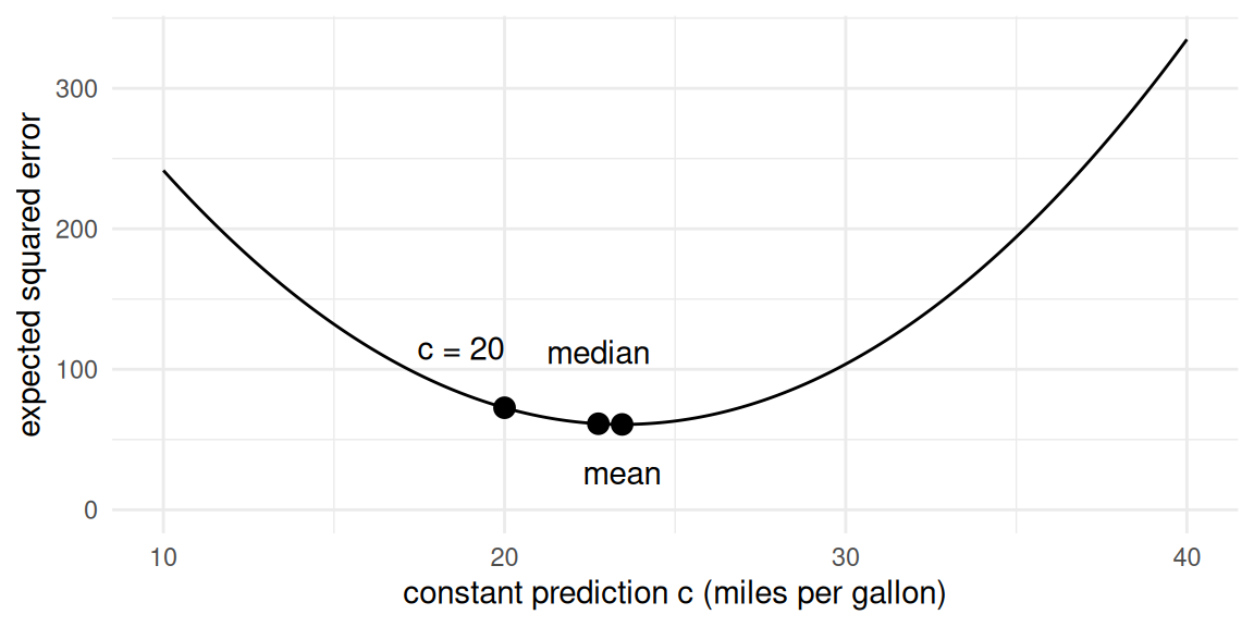
Example 10 (The best constant prediction of fuel economy) Take the 392 cars in the Auto data described on the limit theorems page as the whole population, and predict the fuel economy (mpg) of a car drawn at random with one number \(c\). The code below computes the expected squared error of three constants, and sets each beside the right side of Equation 1.
auto <- readr::read_csv("data/auto.csv", show_col_types = FALSE)
mpg <- auto$mpg
mu <- mean(mpg)
squared_deviations <- (mpg - mu)^2
sigma2 <- mean(squared_deviations)
median_mpg <- median(mpg)
c_values <- c(mean = mu, median = median_mpg, twenty = 20)
constants <- names(c_values)
errors_by_car <- outer(mpg, c_values, "-")
squared_errors <- errors_by_car^2
errors <- colMeans(squared_errors)
shift_squared <- (mu - c_values)^2
tibble::tibble(
constant = constants,
c = c_values,
expected_squared_error = errors,
decomposition = sigma2 + shift_squared
)Figure 2 plots the expected squared error of every constant from 10 to 40 against \(c\), and marks the three constants in the table.
Show code
c_grid <- seq(10, 40, length.out = 301)
grid_deviations <- outer(mpg, c_grid, "-")
grid_squared <- grid_deviations^2
grid_errors <- colMeans(grid_squared)
curve <- tibble::tibble(c = c_grid, expected_squared_error = grid_errors)
point_labels <- c("mean", "median", "c = 20")
label_hjust <- c(0.5, 0.5, 1)
label_vjust <- c(2.5, -2.5, -2)
marked <- tibble::tibble(
point_label = point_labels,
c = c_values,
expected_squared_error = errors,
label_hjust = label_hjust,
label_vjust = label_vjust
)
curve_aes <- ggplot2::aes(x = c, y = expected_squared_error)
label_aes <- ggplot2::aes(
label = point_label,
hjust = label_hjust,
vjust = label_vjust
)
curve |>
ggplot2::ggplot() +
curve_aes +
ggplot2::geom_line() +
ggplot2::geom_point(data = marked, size = 3) +
ggplot2::geom_text(label_aes, data = marked) +
ggplot2::labs(
x = "constant prediction c (miles per gallon)",
y = "expected squared error"
) +
ggplot2::expand_limits(y = 0) +
ggplot2::theme_minimal()The two columns agree, as Theorem 4 says. The mean, 23.45, has the smallest expected squared error, 60.76, which is the variance of mpg over these cars (divisor the number of cars, not one fewer), as Corollary 1 says; the median and \(c = 20\) are each worse by \({\mathopen{}\left(\mu- c\right)\mathclose{}}^{2}\).
4 Independent noise plus a random variable
4.1 Mean-zero noise model
Measurement noise is almost always modeled as a random variable \(\varepsilon\) with mean zero and variance \(\sigma^2\).
Remark 1 (Mean zero is a parametrization choice). Mean zero is a parametrization choice, not a substantive assumption. In \(Y = f(x) + \varepsilon\), moving a constant from \(\varepsilon\) into \(f(x)\) changes the split but not the distribution of \(Y\), so the data identify only the sum \(f(x) + {\mathbb{E}\mathopen{}\left[\varepsilon\right]\mathclose{}}\), the mean of \(Y\) at \(x\). Requiring \({\mathbb{E}\mathopen{}\left[\varepsilon\right]\mathclose{}} = 0\) picks the one split in which \(f(x)\) is that mean. This loses no generality when the model for \(f\) can absorb a constant, as any model with an intercept can. It restricts the model only when \(f\) cannot absorb one, as in a regression through the origin.
Mean zero gives one identity, used repeatedly across statistical modeling and machine learning.
Exercise 1 (The average squared error of pure noise) Let \(\varepsilon\) be a random variable with \(\mathbb{E}[\varepsilon] = 0\) and \({\operatorname{Var}\mathopen{}\left(\varepsilon\right)\mathclose{}} = \sigma^2\).
Find \(\mathbb{E}[\varepsilon^2]\) in terms of \(\sigma^2\), and say which earlier result you used.
Theorem 5 (The second moment of mean-zero noise) Let \(\varepsilon\) be a random variable with \(\mathbb{E}[\varepsilon] = 0\) and \({\operatorname{Var}\mathopen{}\left(\varepsilon\right)\mathclose{}} = \sigma^2\). Then
\[\mathbb{E}[\varepsilon^2] = \sigma^2\]
Proof. This is the solution to Exercise 1, worked in Solution 1. It rearranges Theorem 2, using \(\mathbb{E}[\varepsilon] = 0\).
Theorem 6 (The second moment of independent noise plus a random variable) Let \(\varepsilon\) be a random variable with \({\mathbb{E}\mathopen{}\left[\varepsilon\right]\mathclose{}} = 0\) and \({\operatorname{Var}\mathopen{}\left(\varepsilon\right)\mathclose{}} = \sigma^2\). Let \(X\) be a random variable with \({\mathbb{E}\mathopen{}\left[X^2\right]\mathclose{}} < \infty\) that is independent of \(\varepsilon\). Then
\[{\mathbb{E}\mathopen{}\left[\mathopen{}\left(\varepsilon+ X\right)\mathclose{}^2\right]\mathclose{}} = \sigma^2+ {\operatorname{Var}\mathopen{}\left(X\right)\mathclose{}} + {\mathopen{}\left({\mathbb{E}\mathopen{}\left[X\right]\mathclose{}}\right)\mathclose{}}^{2}\]
Proof. Expanding the square and using linearity of expectation, first for the expectation of a sum and then for a constant factor,
\[ \begin{aligned} {\mathbb{E}\mathopen{}\left[\mathopen{}\left(\varepsilon+ X\right)\mathclose{}^2\right]\mathclose{}} &= {\mathbb{E}\mathopen{}\left[\varepsilon^2 + 2 \varepsilon X+ X^2\right]\mathclose{}} && \text{(expand: } \mathopen{}\left(a + b\right)\mathclose{}^2 = a^2 + 2ab + b^2 \text{)} \\ &= {\mathbb{E}\mathopen{}\left[\varepsilon^2\right]\mathclose{}} + {\mathbb{E}\mathopen{}\left[2 \varepsilon X\right]\mathclose{}} + {\mathbb{E}\mathopen{}\left[X^2\right]\mathclose{}} && \text{(expectation of a sum)} \\ &= {\mathbb{E}\mathopen{}\left[\varepsilon^2\right]\mathclose{}} + 2{\mathbb{E}\mathopen{}\left[\varepsilon X\right]\mathclose{}} + {\mathbb{E}\mathopen{}\left[X^2\right]\mathclose{}} && \text{(constant factor 2)} \end{aligned} \]
Each of the three terms is evaluated in turn.
\({\mathbb{E}\mathopen{}\left[\varepsilon^2\right]\mathclose{}} = \sigma^2\), by Theorem 5.
Because \(\varepsilon\) and \(X\) are independent, the expectation of the product is the product of the expectations:
\[ \begin{aligned} {\mathbb{E}\mathopen{}\left[\varepsilon X\right]\mathclose{}} &= {\mathbb{E}\mathopen{}\left[\varepsilon\right]\mathclose{}}{\mathbb{E}\mathopen{}\left[X\right]\mathclose{}} && \text{(independence)} \\ &= 0 \cdot {\mathbb{E}\mathopen{}\left[X\right]\mathclose{}} && \text{(} {\mathbb{E}\mathopen{}\left[\varepsilon\right]\mathclose{}} = 0 \text{)} \\ &= 0 && \text{(zero times a number)} \end{aligned} \]
\({\mathbb{E}\mathopen{}\left[X^2\right]\mathclose{}} = {\operatorname{Var}\mathopen{}\left(X\right)\mathclose{}} + {\mathopen{}\left({\mathbb{E}\mathopen{}\left[X\right]\mathclose{}}\right)\mathclose{}}^{2}\), by Theorem 2.
Substituting the three terms gives
\[ \begin{aligned} {\mathbb{E}\mathopen{}\left[\mathopen{}\left(\varepsilon+ X\right)\mathclose{}^2\right]\mathclose{}} &= \sigma^2+ 2 \cdot 0 + \mathopen{}\left({\operatorname{Var}\mathopen{}\left(X\right)\mathclose{}} + {\mathopen{}\left({\mathbb{E}\mathopen{}\left[X\right]\mathclose{}}\right)\mathclose{}}^{2}\right)\mathclose{} && \text{(the three terms above)} \\ &= \sigma^2+ {\operatorname{Var}\mathopen{}\left(X\right)\mathclose{}} + {\mathopen{}\left({\mathbb{E}\mathopen{}\left[X\right]\mathclose{}}\right)\mathclose{}}^{2} && \text{(drop } 2 \cdot 0 \text{)} \end{aligned} \]
Remark (Use in statistics and machine learning). Let \(\varepsilon\) be the noise in a new outcome \(Y\), and let \(X\) be the difference between the true mean \(\mu= {\mathbb{E}\mathopen{}\left[Y\right]\mathclose{}}\) and a prediction \(\hat{y}\):
\[X\stackrel{\text{def}}{=}\mu- \hat{y}\]
The mean of \(X\) is minus the bias of the prediction:
\[ \begin{aligned} {\mathbb{E}\mathopen{}\left[X\right]\mathclose{}} &= {\mathbb{E}\mathopen{}\left[\mu- \hat{y}\right]\mathclose{}} && \text{(definition of } X\text{)} \\ &= \mu- {\mathbb{E}\mathopen{}\left[\hat{y}\right]\mathclose{}} && \text{(expectation of a difference; } \mu\text{ is a constant)} \\ &= -\mathopen{}\left({\mathbb{E}\mathopen{}\left[\hat{y}\right]\mathclose{}} - \mu\right)\mathclose{} && \text{(factor out } -1 \text{)} \\ &= -{\operatorname{Bias}\mathopen{}\left(\hat{y}\right)\mathclose{}} && \text{(definition of bias)} \end{aligned} \]
The variance of \(X\) is the variance of the prediction:
\[ \begin{aligned} {\operatorname{Var}\mathopen{}\left(X\right)\mathclose{}} &= {\operatorname{Var}\mathopen{}\left(\mu- \hat{y}\right)\mathclose{}} && \text{(definition of } X\text{)} \\ &= {\operatorname{Var}\mathopen{}\left(\hat{y}\right)\mathclose{}} && \text{(a constant shifts a variable without changing its variance, and a sign flip does not change it either)} \end{aligned} \]
Substituting these two results into the theorem, with \({\mathopen{}\left(-{\operatorname{Bias}\mathopen{}\left(\hat{y}\right)\mathclose{}}\right)\mathclose{}}^{2} = {\mathopen{}\left({\operatorname{Bias}\mathopen{}\left(\hat{y}\right)\mathclose{}}\right)\mathclose{}}^{2}\), gives the squared prediction error of the new outcome as
\[ {\mathbb{E}\mathopen{}\left[{\mathopen{}\left(\varepsilon+ X\right)\mathclose{}}^{2}\right]\mathclose{}} = \sigma^2+ {\operatorname{Var}\mathopen{}\left(\hat{y}\right)\mathclose{}} + {\mathopen{}\left({\operatorname{Bias}\mathopen{}\left(\hat{y}\right)\mathclose{}}\right)\mathclose{}}^{2}, \]
where \(\sigma^2\) is the residual variance. The statistics notes define the bias of a prediction and the training data it depends on, and state this result for predictions as the bias, variance and noise decomposition, with its exercise, worked example and definition of the residual variance.
5 Covariance
Definition 9 (Covariance) The covariance of two random variables \(X\) and \(Y\) with \({\mathbb{E}\mathopen{}\left[X^2\right]\mathclose{}} < \infty\) and \({\mathbb{E}\mathopen{}\left[Y^2\right]\mathclose{}} < \infty\) [3] is:
\[{\operatorname{Cov}\mathopen{}\left(X,Y\right)\mathclose{}} \stackrel{\text{def}}{=}{\mathbb{E}\mathopen{}\left[(X - {\mathbb{E}\mathopen{}\left[X\right]\mathclose{}})(Y - {\mathbb{E}\mathopen{}\left[Y\right]\mathclose{}})\right]\mathclose{}}\]
Theorem 7 (Alternative formula for covariance) \[{\operatorname{Cov}\mathopen{}\left(X,Y\right)\mathclose{}}= {\mathbb{E}\mathopen{}\left[XY\right]\mathclose{}} - {\mathbb{E}\mathopen{}\left[X\right]\mathclose{}} {\mathbb{E}\mathopen{}\left[Y\right]\mathclose{}}\]
Proof. Let \(\mu_X = {\mathbb{E}\mathopen{}\left[X\right]\mathclose{}}\) and \(\mu_Y = {\mathbb{E}\mathopen{}\left[Y\right]\mathclose{}}\) be the population means of \(X\) and \(Y\). They are constants, so linearity of expectation applies with them as coefficients, analogous to the proof of the simplified expression for variance:
\[ \begin{aligned} {\operatorname{Cov}\mathopen{}\left(X,Y\right)\mathclose{}} &\stackrel{\text{def}}{=}{\mathbb{E}\mathopen{}\left[(X-\mu_X)(Y-\mu_Y)\right]\mathclose{}} && \text{(definition of covariance, with population means } \mu_X, \mu_Y \text{)} \\ &= {\mathbb{E}\mathopen{}\left[XY - X\mu_Y - Y\mu_X + \mu_X\mu_Y\right]\mathclose{}} && \text{(expand the product)} \\ &= {\mathbb{E}\mathopen{}\left[XY\right]\mathclose{}} - \mu_Y{\mathbb{E}\mathopen{}\left[X\right]\mathclose{}} - \mu_X{\mathbb{E}\mathopen{}\left[Y\right]\mathclose{}} + \mu_X\mu_Y && \text{(linearity of expectation; } \mu_X, \mu_Y \text{ are constants)} \\ &= {\mathbb{E}\mathopen{}\left[XY\right]\mathclose{}} - \mu_Y\mu_X - \mu_X\mu_Y + \mu_X\mu_Y && \text{(} {\mathbb{E}\mathopen{}\left[X\right]\mathclose{}} = \mu_X \text{ and } {\mathbb{E}\mathopen{}\left[Y\right]\mathclose{}} = \mu_Y \text{)} \\ &= {\mathbb{E}\mathopen{}\left[XY\right]\mathclose{}} - \mu_X\mu_Y && \text{(combine like terms)} \\ &= {\mathbb{E}\mathopen{}\left[XY\right]\mathclose{}} - {\mathbb{E}\mathopen{}\left[X\right]\mathclose{}}{\mathbb{E}\mathopen{}\left[Y\right]\mathclose{}} && \text{(} \mu_X = {\mathbb{E}\mathopen{}\left[X\right]\mathclose{}} \text{ and } \mu_Y = {\mathbb{E}\mathopen{}\left[Y\right]\mathclose{}} \text{)} \end{aligned} \]
Example 11 (Covariance of a binary exposure and outcome) For the joint PMF in Example 4,
\[ \begin{aligned} {\mathbb{E}\mathopen{}\left[XY\right]\mathclose{}} &= \mathbb{P}(X = 1, Y = 1) \\ &= 0.4, \end{aligned} \]
\({\mathbb{E}\mathopen{}\left[X\right]\mathclose{}} = 0.5\), and \({\mathbb{E}\mathopen{}\left[Y\right]\mathclose{}} = 0.7\), so:
\[ \begin{aligned} {\operatorname{Cov}\mathopen{}\left(X,Y\right)\mathclose{}} &= {\mathbb{E}\mathopen{}\left[XY\right]\mathclose{}} - {\mathbb{E}\mathopen{}\left[X\right]\mathclose{}}{\mathbb{E}\mathopen{}\left[Y\right]\mathclose{}} && \text{(alternative formula for covariance)} \\ &= 0.4 - 0.5 \cdot 0.7 && \text{(substitute)} \\ &= 0.05 && \text{(evaluate)} \end{aligned} \]
Proof. Write \(f_X\) and \(f_Y\) for the PMFs or densities of \(X\) and \(Y\), with reference measures \(\mu_X\) and \(\mu_Y\) as in the joint-distribution form of Fubini–Tonelli (counting measure for a discrete variable, Lebesgue measure for a continuous one). Because \(X\) and \(Y\) are independent, \(f_{X,Y}(x, y) = f_X(x)\,f_Y(y)\) is their joint PMF, density, or density-mass function (the factorization in the notes to the definition of independence). First, with \(h(x, y) = \mathopen{}\left|x\right|\mathclose{}\mathopen{}\left|y\right|\mathclose{} \ge 0\) (condition (a)):
\[ \begin{aligned} {\mathbb{E}\mathopen{}\left[\mathopen{}\left|XY\right|\mathclose{}\right]\mathclose{}} &= \int_{\mathcal{R}(X)}\mathopen{}\left(\int_{\mathcal{R}(Y)} \mathopen{}\left|x\right|\mathclose{}\mathopen{}\left|y\right|\mathclose{}\,f_X(x)\,f_Y(y)\,d\mu_Y(y)\right)\mathclose{}\,d\mu_X(x) && \text{(joint-distribution form of Fubini--Tonelli, condition (a))} \\ &= \int_{\mathcal{R}(X)} \mathopen{}\left|x\right|\mathclose{}\,f_X(x)\mathopen{}\left(\int_{\mathcal{R}(Y)} \mathopen{}\left|y\right|\mathclose{}\,f_Y(y)\,d\mu_Y(y)\right)\mathclose{}\,d\mu_X(x) && \text{(} \mathopen{}\left|x\right|\mathclose{}\,f_X(x) \text{ does not depend on } y \text{)} \\ &= \int_{\mathcal{R}(X)} \mathopen{}\left|x\right|\mathclose{}\,f_X(x) \cdot{\mathbb{E}\mathopen{}\left[\mathopen{}\left|Y\right|\mathclose{}\right]\mathclose{}}\,d\mu_X(x) && \text{(LOTUS for } \mathopen{}\left|Y\right|\mathclose{} \text{)} \\ &= {\mathbb{E}\mathopen{}\left[\mathopen{}\left|X\right|\mathclose{}\right]\mathclose{}} \cdot{\mathbb{E}\mathopen{}\left[\mathopen{}\left|Y\right|\mathclose{}\right]\mathclose{}} && \text{(LOTUS for } \mathopen{}\left|X\right|\mathclose{} \text{)} \end{aligned} \]
which is finite, because \(X\) and \(Y\) have defined expectations. So condition (b) holds for \(h(x, y) = xy\), and the same steps without the absolute values give:
\[ \begin{aligned} {\mathbb{E}\mathopen{}\left[XY\right]\mathclose{}} &= \int_{\mathcal{R}(X)}\mathopen{}\left(\int_{\mathcal{R}(Y)} xy\,f_X(x)\,f_Y(y)\,d\mu_Y(y)\right)\mathclose{}\,d\mu_X(x) && \text{(joint-distribution form of Fubini--Tonelli, condition (b))} \\ &= \int_{\mathcal{R}(X)} x\,f_X(x)\mathopen{}\left(\int_{\mathcal{R}(Y)} y\,f_Y(y)\,d\mu_Y(y)\right)\mathclose{}\,d\mu_X(x) && \text{(} x\,f_X(x) \text{ does not depend on } y \text{)} \\ &= \int_{\mathcal{R}(X)} x\,f_X(x) \cdot{\mathbb{E}\mathopen{}\left[Y\right]\mathclose{}}\,d\mu_X(x) && \text{(definition of expectation)} \\ &= {\mathbb{E}\mathopen{}\left[X\right]\mathclose{}} \cdot{\mathbb{E}\mathopen{}\left[Y\right]\mathclose{}} && \text{(definition of expectation)} \end{aligned} \]
Finally, by the alternative formula for covariance:
\[ \begin{aligned} {\operatorname{Cov}\mathopen{}\left(X,Y\right)\mathclose{}} &= {\mathbb{E}\mathopen{}\left[XY\right]\mathclose{}} - {\mathbb{E}\mathopen{}\left[X\right]\mathclose{}}{\mathbb{E}\mathopen{}\left[Y\right]\mathclose{}} && \text{(alternative formula for covariance)} \\ &= {\mathbb{E}\mathopen{}\left[X\right]\mathclose{}}{\mathbb{E}\mathopen{}\left[Y\right]\mathclose{}} - {\mathbb{E}\mathopen{}\left[X\right]\mathclose{}}{\mathbb{E}\mathopen{}\left[Y\right]\mathclose{}} && \text{(} {\mathbb{E}\mathopen{}\left[XY\right]\mathclose{}} = {\mathbb{E}\mathopen{}\left[X\right]\mathclose{}}{\mathbb{E}\mathopen{}\left[Y\right]\mathclose{}} \text{)} \\ &= 0 && \text{(subtract)} \end{aligned} \]
Definition 10 (Correlation) The correlation of two random variables \(X\) and \(Y\) with finite, positive variances is their covariance divided by the product of their standard deviations:
\[{\operatorname{Cor}\mathopen{}\left(X,Y\right)\mathclose{}} \stackrel{\text{def}}{=}\frac{{\operatorname{Cov}\mathopen{}\left(X,Y\right)\mathclose{}}}{{\operatorname{SD}\mathopen{}\left(X\right)\mathclose{}}\,{\operatorname{SD}\mathopen{}\left(Y\right)\mathclose{}}}\]
Remark. Dividing by the standard deviations removes the units of \(X\) and \(Y\). This population correlation is a property of a joint distribution; the sample (Pearson) correlation coefficient computed from data estimates it.
Example 14 (Correlation of a binary exposure and outcome) In Example 11, \({\operatorname{Cov}\mathopen{}\left(X,Y\right)\mathclose{}} = 0.05\), where \(X \sim \operatorname{Ber}(0.5)\) has \({\operatorname{Var}\mathopen{}\left(X\right)\mathclose{}} = 0.25\) (Example 3) and \(Y\) has \({\operatorname{Var}\mathopen{}\left(Y\right)\mathclose{}} = 0.21\) (Example 7), so:
\[ \begin{aligned} {\operatorname{Cor}\mathopen{}\left(X,Y\right)\mathclose{}} &= \frac{{\operatorname{Cov}\mathopen{}\left(X,Y\right)\mathclose{}}}{{\operatorname{SD}\mathopen{}\left(X\right)\mathclose{}}\,{\operatorname{SD}\mathopen{}\left(Y\right)\mathclose{}}} && \text{(definition of correlation)} \\ &= \frac{0.05}{\sqrt{0.25} \cdot\sqrt{0.21}} && \text{(substitute; } {\operatorname{SD}\mathopen{}\left(\cdot\right)\mathclose{}} = \sqrt{{\operatorname{Var}\mathopen{}\left(\cdot\right)\mathclose{}}} \text{)} \\ &\approx \frac{0.05}{0.5 \cdot 0.458} && \text{(evaluate the square roots)} \\ &\approx 0.218 && \text{(divide)} \end{aligned} \]
Remark. Theorem 8 says independent random variables are uncorrelated, and Example 13 shows the converse fails.
Proof. By Definition 10, \({\operatorname{Cor}\mathopen{}\left(X,Y\right)\mathclose{}} = {\operatorname{Cov}\mathopen{}\left(X,Y\right)\mathclose{}} / \mathopen{}\left({\operatorname{SD}\mathopen{}\left(X\right)\mathclose{}}\,{\operatorname{SD}\mathopen{}\left(Y\right)\mathclose{}}\right)\mathclose{}\), and \({\operatorname{SD}\mathopen{}\left(X\right)\mathclose{}}\,{\operatorname{SD}\mathopen{}\left(Y\right)\mathclose{}} > 0\) because both variances are positive, so \({\operatorname{Cor}\mathopen{}\left(X,Y\right)\mathclose{}} = 0\) if and only if \({\operatorname{Cov}\mathopen{}\left(X,Y\right)\mathclose{}} = 0\), which is Definition 11.
Definition 12 (Conditional covariance) The conditional covariance of \(Y\) and \(Z\) given \(X = x\) is their covariance under their conditional distribution given \(X = x\):
\[{\operatorname{Cov}\mathopen{}\left(Y,Z \mid X = x\right)\mathclose{}} \stackrel{\text{def}}{=}{\mathbb{E}\mathopen{}\left[\mathopen{}\left(Y-{\mathbb{E}\mathopen{}\left[Y \mid X = x\right]\mathclose{}}\right)\mathclose{}\mathopen{}\left(Z-{\mathbb{E}\mathopen{}\left[Z \mid X = x\right]\mathclose{}}\right)\mathclose{} \mid X = x\right]\mathclose{}}\]
Evaluating this function of \(x\) at \(X\) gives the random variable \({\operatorname{Cov}\mathopen{}\left(Y,Z \mid X\right)\mathclose{}}\).
Example 16 (Conditional covariance of a variable with itself) Taking \(Z = Y\) in Definition 12 gives the conditional variance: \({\operatorname{Cov}\mathopen{}\left(Y,Y \mid X = x\right)\mathclose{}} = {\operatorname{Var}\mathopen{}\left(Y \mid X = x\right)\mathclose{}}\). In Example 4, for example, \({\operatorname{Cov}\mathopen{}\left(Y,Y \mid X = 0\right)\mathclose{}} = 0.24\).
Theorem 9 (Law of total covariance (covariance decomposition formula, conditional covariance formula)) For random variables \(X\), \(Y\), and \(Z\) with \({\mathbb{E}\mathopen{}\left[Y^2\right]\mathclose{}} < \infty\) and \({\mathbb{E}\mathopen{}\left[Z^2\right]\mathclose{}} < \infty\):
\[{\operatorname{Cov}\mathopen{}\left(Y,Z\right)\mathclose{}} = {\mathbb{E}\mathopen{}\left[{\operatorname{Cov}\mathopen{}\left(Y,Z \mid X\right)\mathclose{}}\right]\mathclose{}} + {\operatorname{Cov}\mathopen{}\left({\mathbb{E}\mathopen{}\left[Y \mid X\right]\mathclose{}}, {\mathbb{E}\mathopen{}\left[Z \mid X\right]\mathclose{}}\right)\mathclose{}}\]
Proof. The proof follows the proof of the law of total variance, which is the special case \(Z = Y\). Write \(m_Y(X) \stackrel{\text{def}}{=}{\mathbb{E}\mathopen{}\left[Y \mid X\right]\mathclose{}}\), \(m_Z(X) \stackrel{\text{def}}{=}{\mathbb{E}\mathopen{}\left[Z \mid X\right]\mathclose{}}\), \(\mu_Y \stackrel{\text{def}}{=}{\mathbb{E}\mathopen{}\left[Y\right]\mathclose{}}\), and \(\mu_Z \stackrel{\text{def}}{=}{\mathbb{E}\mathopen{}\left[Z\right]\mathclose{}}\). Adding and subtracting \(m_Y(X)\) and \(m_Z(X)\) inside the deviations:
\[ \begin{aligned} {\operatorname{Cov}\mathopen{}\left(Y,Z\right)\mathclose{}} &= {\mathbb{E}\mathopen{}\left[\mathopen{}\left(Y - \mu_Y\right)\mathclose{}\mathopen{}\left(Z - \mu_Z\right)\mathclose{}\right]\mathclose{}} && \text{(definition of covariance)} \\ &= {\mathbb{E}\mathopen{}\left[\mathopen{}\left(\mathopen{}\left[Y - m_Y(X)\right]\mathclose{} + \mathopen{}\left[m_Y(X) - \mu_Y\right]\mathclose{}\right)\mathclose{}\mathopen{}\left(\mathopen{}\left[Z - m_Z(X)\right]\mathclose{} + \mathopen{}\left[m_Z(X) - \mu_Z\right]\mathclose{}\right)\mathclose{}\right]\mathclose{}} && \text{(add and subtract)} \\ &= {\mathbb{E}\mathopen{}\left[\mathopen{}\left[Y - m_Y(X)\right]\mathclose{}\mathopen{}\left[Z - m_Z(X)\right]\mathclose{}\right]\mathclose{}} + {\mathbb{E}\mathopen{}\left[\mathopen{}\left[Y - m_Y(X)\right]\mathclose{}\mathopen{}\left[m_Z(X) - \mu_Z\right]\mathclose{}\right]\mathclose{}} \\&\quad + {\mathbb{E}\mathopen{}\left[\mathopen{}\left[m_Y(X) - \mu_Y\right]\mathclose{}\mathopen{}\left[Z - m_Z(X)\right]\mathclose{}\right]\mathclose{}} + {\mathbb{E}\mathopen{}\left[\mathopen{}\left[m_Y(X) - \mu_Y\right]\mathclose{}\mathopen{}\left[m_Z(X) - \mu_Z\right]\mathclose{}\right]\mathclose{}} && \text{(expand the product; linearity of expectation)} \end{aligned} \]
The two middle terms are 0, by the same steps as the cross term in the proof of Theorem 3: condition on \(X\) by the law of iterated expectations, factor out the function of \(X\) (pull-out property), and use \({\mathbb{E}\mathopen{}\left[Y - m_Y(X) \mid X\right]\mathclose{}} = 0\) (or \({\mathbb{E}\mathopen{}\left[Z - m_Z(X) \mid X\right]\mathclose{}} = 0\)), which follows from linearity of conditional expectation. For the first term:
\[ \begin{aligned} {\mathbb{E}\mathopen{}\left[\mathopen{}\left[Y - m_Y(X)\right]\mathclose{}\mathopen{}\left[Z - m_Z(X)\right]\mathclose{}\right]\mathclose{}} &= {\mathbb{E}\mathopen{}\left[{\mathbb{E}\mathopen{}\left[\mathopen{}\left[Y - m_Y(X)\right]\mathclose{}\mathopen{}\left[Z - m_Z(X)\right]\mathclose{} \mid X\right]\mathclose{}}\right]\mathclose{}} && \text{(law of iterated expectations)} \\ &= {\mathbb{E}\mathopen{}\left[{\operatorname{Cov}\mathopen{}\left(Y,Z \mid X\right)\mathclose{}}\right]\mathclose{}} && \text{(definition of conditional covariance)} \end{aligned} \]
For the last term, the law of iterated expectations gives \({\mathbb{E}\mathopen{}\left[m_Y(X)\right]\mathclose{}} = \mu_Y\) and \({\mathbb{E}\mathopen{}\left[m_Z(X)\right]\mathclose{}} = \mu_Z\), so:
\[ \begin{aligned} {\mathbb{E}\mathopen{}\left[\mathopen{}\left[m_Y(X) - \mu_Y\right]\mathclose{}\mathopen{}\left[m_Z(X) - \mu_Z\right]\mathclose{}\right]\mathclose{}} &= {\mathbb{E}\mathopen{}\left[\mathopen{}\left[m_Y(X) - {\mathbb{E}\mathopen{}\left[m_Y(X)\right]\mathclose{}}\right]\mathclose{}\mathopen{}\left[m_Z(X) - {\mathbb{E}\mathopen{}\left[m_Z(X)\right]\mathclose{}}\right]\mathclose{}\right]\mathclose{}} && \text{(substitute the means)} \\ &= {\operatorname{Cov}\mathopen{}\left(m_Y(X), m_Z(X)\right)\mathclose{}} && \text{(definition of covariance)} \\ &= {\operatorname{Cov}\mathopen{}\left({\mathbb{E}\mathopen{}\left[Y \mid X\right]\mathclose{}}, {\mathbb{E}\mathopen{}\left[Z \mid X\right]\mathclose{}}\right)\mathclose{}} && \text{(definitions of } m_Y, m_Z \text{)} \end{aligned} \]
Adding the four terms gives the result.
Lemma 2 (The covariance of a variable with itself is its variance) For any random variable \(X\) with \({\mathbb{E}\mathopen{}\left[X^2\right]\mathclose{}} < \infty\):
\[{\operatorname{Cov}\mathopen{}\left(X,X\right)\mathclose{}} = {\operatorname{Var}\mathopen{}\left(X\right)\mathclose{}}\]
Proof. By the alternative formula for covariance:
\[ \begin{aligned} {\operatorname{Cov}\mathopen{}\left(X,X\right)\mathclose{}} &= {\mathbb{E}\mathopen{}\left[XX\right]\mathclose{}} - {\mathbb{E}\mathopen{}\left[X\right]\mathclose{}}{\mathbb{E}\mathopen{}\left[X\right]\mathclose{}} && \text{(alternative formula for covariance, with } Y = X \text{)} \\&= {\mathbb{E}\mathopen{}\left[X^2\right]\mathclose{}} - {\mathopen{}\left({\mathbb{E}\mathopen{}\left[X\right]\mathclose{}}\right)\mathclose{}}^{2} && \text{(} XX = X^2 \text{)} \\&= {\operatorname{Var}\mathopen{}\left(X\right)\mathclose{}} && \text{(simplified expression for variance)} \end{aligned} \]
Definition 13 (Variance/covariance of a \(p \times 1\) random vector) For a \(p \times 1\) dimensional random vector \(\mathord{\smash[b]{\underset{\raise.3ex\hbox{$\scriptstyle\sim$}}{X}}\vphantom{X}}\),
\[ \begin{aligned} {\operatorname{Var}\mathopen{}\left(\mathord{\smash[b]{\underset{\raise.3ex\hbox{$\scriptstyle\sim$}}{X}}\vphantom{X}}\right)\mathclose{}} &\stackrel{\text{def}}{=}{\operatorname{Cov}\mathopen{}\left(\mathord{\smash[b]{\underset{\raise.3ex\hbox{$\scriptstyle\sim$}}{X}}\vphantom{X}}\right)\mathclose{}} \\ &\stackrel{\text{def}}{=}{\mathbb{E}\mathopen{}\left[\mathopen{}\left(\mathord{\smash[b]{\underset{\raise.3ex\hbox{$\scriptstyle\sim$}}{X}}\vphantom{X}}- \mathbb{E}\mathord{\smash[b]{\underset{\raise.3ex\hbox{$\scriptstyle\sim$}}{X}}\vphantom{X}}\right)\mathclose{} {\mathopen{}\left(\mathord{\smash[b]{\underset{\raise.3ex\hbox{$\scriptstyle\sim$}}{X}}\vphantom{X}}- \mathbb{E}\mathord{\smash[b]{\underset{\raise.3ex\hbox{$\scriptstyle\sim$}}{X}}\vphantom{X}}\right)\mathclose{}}^{\top}\right]\mathclose{}} \end{aligned} \]
Theorem 10 (Elements of the variance-covariance matrix are pairwise covariances) For a \(p \times 1\) random vector \(\mathord{\smash[b]{\underset{\raise.3ex\hbox{$\scriptstyle\sim$}}{X}}\vphantom{X}}= {(X_1, \ldots, X_p)}^{\top}\), the \((i,j)\)-th element of \({\operatorname{Var}\mathopen{}\left(\mathord{\smash[b]{\underset{\raise.3ex\hbox{$\scriptstyle\sim$}}{X}}\vphantom{X}}\right)\mathclose{}}\) is \({\operatorname{Cov}\mathopen{}\left(X_i, X_j\right)\mathclose{}}\):
\[ {\operatorname{Var}\mathopen{}\left(\mathord{\smash[b]{\underset{\raise.3ex\hbox{$\scriptstyle\sim$}}{X}}\vphantom{X}}\right)\mathclose{}}= \begin{pmatrix} {\operatorname{Var}\mathopen{}\left(X_1\right)\mathclose{}} & {\operatorname{Cov}\mathopen{}\left(X_1, X_2\right)\mathclose{}} & \cdots & {\operatorname{Cov}\mathopen{}\left(X_1, X_p\right)\mathclose{}} \\ {\operatorname{Cov}\mathopen{}\left(X_2, X_1\right)\mathclose{}} & {\operatorname{Var}\mathopen{}\left(X_2\right)\mathclose{}} & \cdots & {\operatorname{Cov}\mathopen{}\left(X_2, X_p\right)\mathclose{}} \\ \vdots & \vdots & \ddots & \vdots \\ {\operatorname{Cov}\mathopen{}\left(X_p, X_1\right)\mathclose{}} & {\operatorname{Cov}\mathopen{}\left(X_p, X_2\right)\mathclose{}} & \cdots & {\operatorname{Var}\mathopen{}\left(X_p\right)\mathclose{}} \end{pmatrix} \]
Proof. Let \(\mu_i = {\mathbb{E}\mathopen{}\left[X_i\right]\mathclose{}}\) for \(i = 1, \ldots, p\), so \(\mathbb{E}\mathord{\smash[b]{\underset{\raise.3ex\hbox{$\scriptstyle\sim$}}{X}}\vphantom{X}}= {(\mu_1, \ldots, \mu_p)}^{\top}\). By Definition 13:
\[ \begin{aligned} {\operatorname{Var}\mathopen{}\left(\mathord{\smash[b]{\underset{\raise.3ex\hbox{$\scriptstyle\sim$}}{X}}\vphantom{X}}\right)\mathclose{}} &= {\mathbb{E}\mathopen{}\left[ \mathopen{}\left(\mathord{\smash[b]{\underset{\raise.3ex\hbox{$\scriptstyle\sim$}}{X}}\vphantom{X}}- \mathbb{E}\mathord{\smash[b]{\underset{\raise.3ex\hbox{$\scriptstyle\sim$}}{X}}\vphantom{X}}\right)\mathclose{} {\mathopen{}\left(\mathord{\smash[b]{\underset{\raise.3ex\hbox{$\scriptstyle\sim$}}{X}}\vphantom{X}}- \mathbb{E}\mathord{\smash[b]{\underset{\raise.3ex\hbox{$\scriptstyle\sim$}}{X}}\vphantom{X}}\right)\mathclose{}}^{\top} \right]\mathclose{}} \\ &= {\mathbb{E}\mathopen{}\left[ \begin{pmatrix}X_1 - \mu_1 \\ \vdots \\ X_p - \mu_p\end{pmatrix} \begin{pmatrix}X_1 - \mu_1 & \cdots & X_p - \mu_p\end{pmatrix} \right]\mathclose{}} \\ &= {\mathbb{E}\mathopen{}\left[ \begin{pmatrix} (X_1 - \mu_1)(X_1 - \mu_1) & \cdots & (X_1 - \mu_1)(X_p - \mu_p) \\ \vdots & \ddots & \vdots \\ (X_p - \mu_p)(X_1 - \mu_1) & \cdots & (X_p - \mu_p)(X_p - \mu_p) \end{pmatrix} \right]\mathclose{}} \\ &= \begin{pmatrix} {\mathbb{E}\mathopen{}\left[(X_1 - \mu_1)(X_1 - \mu_1)\right]\mathclose{}} & \cdots & {\mathbb{E}\mathopen{}\left[(X_1 - \mu_1)(X_p - \mu_p)\right]\mathclose{}} \\ \vdots & \ddots & \vdots \\ {\mathbb{E}\mathopen{}\left[(X_p - \mu_p)(X_1 - \mu_1)\right]\mathclose{}} & \cdots & {\mathbb{E}\mathopen{}\left[(X_p - \mu_p)(X_p - \mu_p)\right]\mathclose{}} \end{pmatrix} \\ &= \begin{pmatrix} {\operatorname{Cov}\mathopen{}\left(X_1, X_1\right)\mathclose{}} & \cdots & {\operatorname{Cov}\mathopen{}\left(X_1, X_p\right)\mathclose{}} \\ \vdots & \ddots & \vdots \\ {\operatorname{Cov}\mathopen{}\left(X_p, X_1\right)\mathclose{}} & \cdots & {\operatorname{Cov}\mathopen{}\left(X_p, X_p\right)\mathclose{}} \end{pmatrix} \\ &= \begin{pmatrix} {\operatorname{Var}\mathopen{}\left(X_1\right)\mathclose{}} & \cdots & {\operatorname{Cov}\mathopen{}\left(X_1, X_p\right)\mathclose{}} \\ \vdots & \ddots & \vdots \\ {\operatorname{Cov}\mathopen{}\left(X_p, X_1\right)\mathclose{}} & \cdots & {\operatorname{Var}\mathopen{}\left(X_p\right)\mathclose{}} \end{pmatrix} \end{aligned} \]
where:
- the step from the third to fourth line uses the expectation of a random matrix,
- the step from the fourth to fifth line uses Definition 9, and
- the last step uses Lemma 2.
Theorem 11 (Alternate expression for variance of a random vector) \[ \begin{aligned} {\operatorname{Var}\mathopen{}\left(\mathord{\smash[b]{\underset{\raise.3ex\hbox{$\scriptstyle\sim$}}{X}}\vphantom{X}}\right)\mathclose{}} &= {\mathbb{E}\mathopen{}\left[\mathord{\smash[b]{\underset{\raise.3ex\hbox{$\scriptstyle\sim$}}{X}}\vphantom{X}}{\mathord{\smash[b]{\underset{\raise.3ex\hbox{$\scriptstyle\sim$}}{X}}\vphantom{X}}}^{\top}\right]\mathclose{}} - \mathopen{}\left(\mathbb{E}\mathord{\smash[b]{\underset{\raise.3ex\hbox{$\scriptstyle\sim$}}{X}}\vphantom{X}}\right)\mathclose{} {\mathopen{}\left(\mathbb{E}\mathord{\smash[b]{\underset{\raise.3ex\hbox{$\scriptstyle\sim$}}{X}}\vphantom{X}}\right)\mathclose{}}^{\top} \end{aligned} \]
Proof. \[ \begin{aligned} {\operatorname{Var}\mathopen{}\left(\mathord{\smash[b]{\underset{\raise.3ex\hbox{$\scriptstyle\sim$}}{X}}\vphantom{X}}\right)\mathclose{}} &= {\mathbb{E}\mathopen{}\left[ \mathopen{}\left(\mathord{\smash[b]{\underset{\raise.3ex\hbox{$\scriptstyle\sim$}}{X}}\vphantom{X}}- \mathbb{E}\mathord{\smash[b]{\underset{\raise.3ex\hbox{$\scriptstyle\sim$}}{X}}\vphantom{X}}\right)\mathclose{} {\mathopen{}\left(\mathord{\smash[b]{\underset{\raise.3ex\hbox{$\scriptstyle\sim$}}{X}}\vphantom{X}}- \mathbb{E}\mathord{\smash[b]{\underset{\raise.3ex\hbox{$\scriptstyle\sim$}}{X}}\vphantom{X}}\right)\mathclose{}}^{\top} \right]\mathclose{}} && \text{(definition)} \\ &= {\mathbb{E}\mathopen{}\left[ \mathord{\smash[b]{\underset{\raise.3ex\hbox{$\scriptstyle\sim$}}{X}}\vphantom{X}}{\mathord{\smash[b]{\underset{\raise.3ex\hbox{$\scriptstyle\sim$}}{X}}\vphantom{X}}}^{\top} - \mathord{\smash[b]{\underset{\raise.3ex\hbox{$\scriptstyle\sim$}}{X}}\vphantom{X}}{\mathopen{}\left(\mathbb{E}\mathord{\smash[b]{\underset{\raise.3ex\hbox{$\scriptstyle\sim$}}{X}}\vphantom{X}}\right)\mathclose{}}^{\top} - \mathopen{}\left(\mathbb{E}\mathord{\smash[b]{\underset{\raise.3ex\hbox{$\scriptstyle\sim$}}{X}}\vphantom{X}}\right)\mathclose{} {\mathord{\smash[b]{\underset{\raise.3ex\hbox{$\scriptstyle\sim$}}{X}}\vphantom{X}}}^{\top} + \mathopen{}\left(\mathbb{E}\mathord{\smash[b]{\underset{\raise.3ex\hbox{$\scriptstyle\sim$}}{X}}\vphantom{X}}\right)\mathclose{} {\mathopen{}\left(\mathbb{E}\mathord{\smash[b]{\underset{\raise.3ex\hbox{$\scriptstyle\sim$}}{X}}\vphantom{X}}\right)\mathclose{}}^{\top} \right]\mathclose{}} && \text{(expand the product)} \\ &= {\mathbb{E}\mathopen{}\left[\mathord{\smash[b]{\underset{\raise.3ex\hbox{$\scriptstyle\sim$}}{X}}\vphantom{X}}{\mathord{\smash[b]{\underset{\raise.3ex\hbox{$\scriptstyle\sim$}}{X}}\vphantom{X}}}^{\top}\right]\mathclose{}} - \mathopen{}\left(\mathbb{E}\mathord{\smash[b]{\underset{\raise.3ex\hbox{$\scriptstyle\sim$}}{X}}\vphantom{X}}\right)\mathclose{} {\mathopen{}\left(\mathbb{E}\mathord{\smash[b]{\underset{\raise.3ex\hbox{$\scriptstyle\sim$}}{X}}\vphantom{X}}\right)\mathclose{}}^{\top} - \mathopen{}\left(\mathbb{E}\mathord{\smash[b]{\underset{\raise.3ex\hbox{$\scriptstyle\sim$}}{X}}\vphantom{X}}\right)\mathclose{} {\mathopen{}\left(\mathbb{E}\mathord{\smash[b]{\underset{\raise.3ex\hbox{$\scriptstyle\sim$}}{X}}\vphantom{X}}\right)\mathclose{}}^{\top} + \mathopen{}\left(\mathbb{E}\mathord{\smash[b]{\underset{\raise.3ex\hbox{$\scriptstyle\sim$}}{X}}\vphantom{X}}\right)\mathclose{} {\mathopen{}\left(\mathbb{E}\mathord{\smash[b]{\underset{\raise.3ex\hbox{$\scriptstyle\sim$}}{X}}\vphantom{X}}\right)\mathclose{}}^{\top} && \text{(linearity, element-wise; } \mathbb{E}\mathord{\smash[b]{\underset{\raise.3ex\hbox{$\scriptstyle\sim$}}{X}}\vphantom{X}}\text{ is constant)} \\ &= {\mathbb{E}\mathopen{}\left[\mathord{\smash[b]{\underset{\raise.3ex\hbox{$\scriptstyle\sim$}}{X}}\vphantom{X}}{\mathord{\smash[b]{\underset{\raise.3ex\hbox{$\scriptstyle\sim$}}{X}}\vphantom{X}}}^{\top}\right]\mathclose{}} - \mathopen{}\left(\mathbb{E}\mathord{\smash[b]{\underset{\raise.3ex\hbox{$\scriptstyle\sim$}}{X}}\vphantom{X}}\right)\mathclose{} {\mathopen{}\left(\mathbb{E}\mathord{\smash[b]{\underset{\raise.3ex\hbox{$\scriptstyle\sim$}}{X}}\vphantom{X}}\right)\mathclose{}}^{\top} && \text{(combine like terms)} \end{aligned} \]
Theorem 12 (Variance of a linear combination) For any vector of random variables \(\mathord{\smash[b]{\underset{\raise.3ex\hbox{$\scriptstyle\sim$}}{X}}\vphantom{X}}= (X_1, \ldots, X_n)\) and corresponding vector of constants \(\mathord{\smash[b]{\underset{\raise.3ex\hbox{$\scriptstyle\sim$}}{a}}\vphantom{a}}= (a_1, \ldots, a_n)\), the variance of their linear combination is:
\[ \begin{aligned} {\operatorname{Var}\mathopen{}\left(\mathord{\smash[b]{\underset{\raise.3ex\hbox{$\scriptstyle\sim$}}{a}}\vphantom{a}}\cdot \mathord{\smash[b]{\underset{\raise.3ex\hbox{$\scriptstyle\sim$}}{X}}\vphantom{X}}\right)\mathclose{}} &= {\operatorname{Var}\mathopen{}\left(\sum_{i=1}^na_i X_i\right)\mathclose{}} \\ &= {\mathord{\smash[b]{\underset{\raise.3ex\hbox{$\scriptstyle\sim$}}{a}}\vphantom{a}}}^{\top} {\operatorname{Var}\mathopen{}\left(\mathord{\smash[b]{\underset{\raise.3ex\hbox{$\scriptstyle\sim$}}{X}}\vphantom{X}}\right)\mathclose{}} \mathord{\smash[b]{\underset{\raise.3ex\hbox{$\scriptstyle\sim$}}{a}}\vphantom{a}} \\ &= \sum_{i=1}^n\sum_{j=1}^n a_i a_j {\operatorname{Cov}\mathopen{}\left(X_i,X_j\right)\mathclose{}} \end{aligned} \]
Proof. Treat \(\mathord{\smash[b]{\underset{\raise.3ex\hbox{$\scriptstyle\sim$}}{a}}\vphantom{a}}\) and \(\mathord{\smash[b]{\underset{\raise.3ex\hbox{$\scriptstyle\sim$}}{X}}\vphantom{X}}\) as \(n \times 1\) column vectors, so
\[ \begin{aligned} \mathord{\smash[b]{\underset{\raise.3ex\hbox{$\scriptstyle\sim$}}{a}}\vphantom{a}}\cdot \mathord{\smash[b]{\underset{\raise.3ex\hbox{$\scriptstyle\sim$}}{X}}\vphantom{X}}&= {\mathord{\smash[b]{\underset{\raise.3ex\hbox{$\scriptstyle\sim$}}{a}}\vphantom{a}}}^{\top}\mathord{\smash[b]{\underset{\raise.3ex\hbox{$\scriptstyle\sim$}}{X}}\vphantom{X}}\\ &= \sum_{i=1}^na_i X_i, \end{aligned} \]
a scalar. By linearity of expectation, \({\mathbb{E}\mathopen{}\left[{\mathord{\smash[b]{\underset{\raise.3ex\hbox{$\scriptstyle\sim$}}{a}}\vphantom{a}}}^{\top}\mathord{\smash[b]{\underset{\raise.3ex\hbox{$\scriptstyle\sim$}}{X}}\vphantom{X}}\right]\mathclose{}} = {\mathord{\smash[b]{\underset{\raise.3ex\hbox{$\scriptstyle\sim$}}{a}}\vphantom{a}}}^{\top}\,\mathbb{E}\mathord{\smash[b]{\underset{\raise.3ex\hbox{$\scriptstyle\sim$}}{X}}\vphantom{X}}\), so:
\[ \begin{aligned} {\operatorname{Var}\mathopen{}\left({\mathord{\smash[b]{\underset{\raise.3ex\hbox{$\scriptstyle\sim$}}{a}}\vphantom{a}}}^{\top}\mathord{\smash[b]{\underset{\raise.3ex\hbox{$\scriptstyle\sim$}}{X}}\vphantom{X}}\right)\mathclose{}} &= {\mathbb{E}\mathopen{}\left[\mathopen{}\left({\mathord{\smash[b]{\underset{\raise.3ex\hbox{$\scriptstyle\sim$}}{a}}\vphantom{a}}}^{\top}\mathord{\smash[b]{\underset{\raise.3ex\hbox{$\scriptstyle\sim$}}{X}}\vphantom{X}}- {\mathord{\smash[b]{\underset{\raise.3ex\hbox{$\scriptstyle\sim$}}{a}}\vphantom{a}}}^{\top}\mathbb{E}\mathord{\smash[b]{\underset{\raise.3ex\hbox{$\scriptstyle\sim$}}{X}}\vphantom{X}}\right)\mathclose{}^2\right]\mathclose{}} && \text{(definition of variance)} \\ &= {\mathbb{E}\mathopen{}\left[\mathopen{}\left({\mathord{\smash[b]{\underset{\raise.3ex\hbox{$\scriptstyle\sim$}}{a}}\vphantom{a}}}^{\top}\mathopen{}\left(\mathord{\smash[b]{\underset{\raise.3ex\hbox{$\scriptstyle\sim$}}{X}}\vphantom{X}}- \mathbb{E}\mathord{\smash[b]{\underset{\raise.3ex\hbox{$\scriptstyle\sim$}}{X}}\vphantom{X}}\right)\mathclose{}\right)\mathclose{}^2\right]\mathclose{}} && \text{(factor out } {\mathord{\smash[b]{\underset{\raise.3ex\hbox{$\scriptstyle\sim$}}{a}}\vphantom{a}}}^{\top} \text{)} \\ &= {\mathbb{E}\mathopen{}\left[{\mathord{\smash[b]{\underset{\raise.3ex\hbox{$\scriptstyle\sim$}}{a}}\vphantom{a}}}^{\top}\mathopen{}\left(\mathord{\smash[b]{\underset{\raise.3ex\hbox{$\scriptstyle\sim$}}{X}}\vphantom{X}}- \mathbb{E}\mathord{\smash[b]{\underset{\raise.3ex\hbox{$\scriptstyle\sim$}}{X}}\vphantom{X}}\right)\mathclose{}{\mathopen{}\left(\mathord{\smash[b]{\underset{\raise.3ex\hbox{$\scriptstyle\sim$}}{X}}\vphantom{X}}- \mathbb{E}\mathord{\smash[b]{\underset{\raise.3ex\hbox{$\scriptstyle\sim$}}{X}}\vphantom{X}}\right)\mathclose{}}^{\top}\mathord{\smash[b]{\underset{\raise.3ex\hbox{$\scriptstyle\sim$}}{a}}\vphantom{a}}\right]\mathclose{}} && \text{(a scalar equals its transpose, so } s^2 = s\,{s}^{\top} \text{)} \\ &= {\mathord{\smash[b]{\underset{\raise.3ex\hbox{$\scriptstyle\sim$}}{a}}\vphantom{a}}}^{\top}\,{\mathbb{E}\mathopen{}\left[\mathopen{}\left(\mathord{\smash[b]{\underset{\raise.3ex\hbox{$\scriptstyle\sim$}}{X}}\vphantom{X}}- \mathbb{E}\mathord{\smash[b]{\underset{\raise.3ex\hbox{$\scriptstyle\sim$}}{X}}\vphantom{X}}\right)\mathclose{}{\mathopen{}\left(\mathord{\smash[b]{\underset{\raise.3ex\hbox{$\scriptstyle\sim$}}{X}}\vphantom{X}}- \mathbb{E}\mathord{\smash[b]{\underset{\raise.3ex\hbox{$\scriptstyle\sim$}}{X}}\vphantom{X}}\right)\mathclose{}}^{\top}\right]\mathclose{}}\,\mathord{\smash[b]{\underset{\raise.3ex\hbox{$\scriptstyle\sim$}}{a}}\vphantom{a}} && \text{(linearity of expectation, element-wise)} \\ &= {\mathord{\smash[b]{\underset{\raise.3ex\hbox{$\scriptstyle\sim$}}{a}}\vphantom{a}}}^{\top} {\operatorname{Var}\mathopen{}\left(\mathord{\smash[b]{\underset{\raise.3ex\hbox{$\scriptstyle\sim$}}{X}}\vphantom{X}}\right)\mathclose{}} \mathord{\smash[b]{\underset{\raise.3ex\hbox{$\scriptstyle\sim$}}{a}}\vphantom{a}} && \text{(variance of a random vector)} \\ &= \sum_{i=1}^n\sum_{j=1}^n a_i a_j {\operatorname{Cov}\mathopen{}\left(X_i,X_j\right)\mathclose{}} && \text{(expand the quadratic form, using the elements of } {\operatorname{Var}\mathopen{}\left(\mathord{\smash[b]{\underset{\raise.3ex\hbox{$\scriptstyle\sim$}}{X}}\vphantom{X}}\right)\mathclose{}} \text{)} \end{aligned} \]
Corollary 3 (Variance of a sum of two random variables) For any two random variables \(X\) and \(Y\) and scalars \(a\) and \(b\):
\[{\operatorname{Var}\mathopen{}\left(aX + bY\right)\mathclose{}} = a^2 {\operatorname{Var}\mathopen{}\left(X\right)\mathclose{}} + b^2 {\operatorname{Var}\mathopen{}\left(Y\right)\mathclose{}} + 2(a \cdot b) {\operatorname{Cov}\mathopen{}\left(X,Y\right)\mathclose{}}\]
Proof. Apply Theorem 12 with \(n=2\), \(X_1 = X\), and \(X_2 = Y\):
\[ \begin{aligned} {\operatorname{Var}\mathopen{}\left(aX+bY\right)\mathclose{}} &= a^2 {\operatorname{Var}\mathopen{}\left(X\right)\mathclose{}} + b^2 {\operatorname{Var}\mathopen{}\left(Y\right)\mathclose{}} + 2ab {\operatorname{Cov}\mathopen{}\left(X,Y\right)\mathclose{}} \end{aligned} \]
Alternatively, by linearity of expectation:
\[ \begin{aligned} {\operatorname{Var}\mathopen{}\left(aX+bY\right)\mathclose{}} &\stackrel{\text{def}}{=}{\mathbb{E}\mathopen{}\left[\mathopen{}\left(aX+bY - {\mathbb{E}\mathopen{}\left[aX+bY\right]\mathclose{}}\right)\mathclose{}^2\right]\mathclose{}} && \text{(definition of variance)} \\ &= {\mathbb{E}\mathopen{}\left[\mathopen{}\left(a(X-\mu_X) + b(Y-\mu_Y)\right)\mathclose{}^2\right]\mathclose{}} && \text{(linearity of expectation, with population means } \mu_X = {\mathbb{E}\mathopen{}\left[X\right]\mathclose{}}, \mu_Y = {\mathbb{E}\mathopen{}\left[Y\right]\mathclose{}} \text{)} \\ &= {\mathbb{E}\mathopen{}\left[a^2(X-\mu_X)^2 + 2(a \cdot b)(X-\mu_X)(Y-\mu_Y) + b^2(Y-\mu_Y)^2\right]\mathclose{}} && \text{(expand the square)} \\ &= a^2{\mathbb{E}\mathopen{}\left[(X-\mu_X)^2\right]\mathclose{}} + 2(a \cdot b){\mathbb{E}\mathopen{}\left[(X-\mu_X)(Y-\mu_Y)\right]\mathclose{}} + b^2{\mathbb{E}\mathopen{}\left[(Y-\mu_Y)^2\right]\mathclose{}} && \text{(linearity of expectation)} \\ &= a^2 {\operatorname{Var}\mathopen{}\left(X\right)\mathclose{}} + 2(a \cdot b) {\operatorname{Cov}\mathopen{}\left(X,Y\right)\mathclose{}} + b^2 {\operatorname{Var}\mathopen{}\left(Y\right)\mathclose{}} && \text{(definitions of variance and covariance)} \end{aligned} \]
Corollary 4 (Variance of a sum of independent random variables) If \(X\) and \(Y\) are independent, each discrete or continuous, with \({\mathbb{E}\mathopen{}\left[X^2\right]\mathclose{}} < \infty\) and \({\mathbb{E}\mathopen{}\left[Y^2\right]\mathclose{}} < \infty\), then:
\[{\operatorname{Var}\mathopen{}\left(X + Y\right)\mathclose{}} = {\operatorname{Var}\mathopen{}\left(X\right)\mathclose{}} + {\operatorname{Var}\mathopen{}\left(Y\right)\mathclose{}}\]
Proof. By Theorem 8, \({\operatorname{Cov}\mathopen{}\left(X,Y\right)\mathclose{}} = 0\). Applying Corollary 3 with
\[ \begin{aligned} a &= b \\ &= 1: \end{aligned} \]
\[ \begin{aligned} {\operatorname{Var}\mathopen{}\left(X + Y\right)\mathclose{}} &= 1^2 {\operatorname{Var}\mathopen{}\left(X\right)\mathclose{}} + 1^2 {\operatorname{Var}\mathopen{}\left(Y\right)\mathclose{}} + 2(1 \cdot 1) {\operatorname{Cov}\mathopen{}\left(X,Y\right)\mathclose{}} && \text{(variance of a sum of two random variables)} \\ &= {\operatorname{Var}\mathopen{}\left(X\right)\mathclose{}} + {\operatorname{Var}\mathopen{}\left(Y\right)\mathclose{}} + 2 {\operatorname{Cov}\mathopen{}\left(X,Y\right)\mathclose{}} && \text{(simplify)} \\ &= {\operatorname{Var}\mathopen{}\left(X\right)\mathclose{}} + {\operatorname{Var}\mathopen{}\left(Y\right)\mathclose{}} && \text{(} {\operatorname{Cov}\mathopen{}\left(X,Y\right)\mathclose{}} = 0 \text{)} \end{aligned} \]
Remark. Corollary 3 is why two variables’ covariance matters for combining them: the covariance term is what separates the variance of their sum from the sum of their variances, and Corollary 4 is the case where that term is 0.
Theorem 13 (A variance matrix is symmetric and positive semidefinite) For a \(p \times 1\) random vector \(\mathord{\smash[b]{\underset{\raise.3ex\hbox{$\scriptstyle\sim$}}{X}}\vphantom{X}}= {(X_1, \ldots, X_p)}^{\top}\) with \({\mathbb{E}\mathopen{}\left[X_i^2\right]\mathclose{}} < \infty\) for every \(i\), \({\operatorname{Var}\mathopen{}\left(\mathord{\smash[b]{\underset{\raise.3ex\hbox{$\scriptstyle\sim$}}{X}}\vphantom{X}}\right)\mathclose{}}\) is symmetric and positive semidefinite: for every \(p \times 1\) vector of constants \(\mathord{\smash[b]{\underset{\raise.3ex\hbox{$\scriptstyle\sim$}}{a}}\vphantom{a}}\),
\[{\mathord{\smash[b]{\underset{\raise.3ex\hbox{$\scriptstyle\sim$}}{a}}\vphantom{a}}}^{\top} {\operatorname{Var}\mathopen{}\left(\mathord{\smash[b]{\underset{\raise.3ex\hbox{$\scriptstyle\sim$}}{X}}\vphantom{X}}\right)\mathclose{}} \mathord{\smash[b]{\underset{\raise.3ex\hbox{$\scriptstyle\sim$}}{a}}\vphantom{a}}\ge 0\]
Proof. By Theorem 10, the \((i,j)\)-th element of \({\operatorname{Var}\mathopen{}\left(\mathord{\smash[b]{\underset{\raise.3ex\hbox{$\scriptstyle\sim$}}{X}}\vphantom{X}}\right)\mathclose{}}\) is \({\operatorname{Cov}\mathopen{}\left(X_i, X_j\right)\mathclose{}}\), and by Definition 9, with \(\mu_i = {\mathbb{E}\mathopen{}\left[X_i\right]\mathclose{}}\):
\[ \begin{aligned} {\operatorname{Cov}\mathopen{}\left(X_i, X_j\right)\mathclose{}} &= {\mathbb{E}\mathopen{}\left[(X_i - \mu_i)(X_j - \mu_j)\right]\mathclose{}} && \text{(definition of covariance)} \\ &= {\mathbb{E}\mathopen{}\left[(X_j - \mu_j)(X_i - \mu_i)\right]\mathclose{}} && \text{(multiplication of numbers is commutative)} \\ &= {\operatorname{Cov}\mathopen{}\left(X_j, X_i\right)\mathclose{}} && \text{(definition of covariance)} \end{aligned} \]
so the \((i,j)\)-th and \((j,i)\)-th elements are equal, and \({\operatorname{Var}\mathopen{}\left(\mathord{\smash[b]{\underset{\raise.3ex\hbox{$\scriptstyle\sim$}}{X}}\vphantom{X}}\right)\mathclose{}}\) is symmetric.
For positive semidefiniteness, let \(Y = {\mathord{\smash[b]{\underset{\raise.3ex\hbox{$\scriptstyle\sim$}}{a}}\vphantom{a}}}^{\top}\mathord{\smash[b]{\underset{\raise.3ex\hbox{$\scriptstyle\sim$}}{X}}\vphantom{X}}\). Then:
\[ \begin{aligned} {\mathord{\smash[b]{\underset{\raise.3ex\hbox{$\scriptstyle\sim$}}{a}}\vphantom{a}}}^{\top} {\operatorname{Var}\mathopen{}\left(\mathord{\smash[b]{\underset{\raise.3ex\hbox{$\scriptstyle\sim$}}{X}}\vphantom{X}}\right)\mathclose{}} \mathord{\smash[b]{\underset{\raise.3ex\hbox{$\scriptstyle\sim$}}{a}}\vphantom{a}} &= {\operatorname{Var}\mathopen{}\left(Y\right)\mathclose{}} && \text{(variance of a linear combination)} \\ &= {\mathbb{E}\mathopen{}\left[(Y - {\mathbb{E}\mathopen{}\left[Y\right]\mathclose{}})^2\right]\mathclose{}} && \text{(definition of variance)} \\ &\ge 0 && \text{(} (Y - {\mathbb{E}\mathopen{}\left[Y\right]\mathclose{}})^2 \ge 0 \text{)} \end{aligned} \]
The first step is Theorem 12. The last step holds because a random variable that is never negative has a non-negative expectation: in the discrete and continuous cases of the definition of expectation, every term of the sum, or the integrand, is non-negative (for the general case, see Billingsley [4]).
Example 17 (Two variance matrices that differ only in sign) Let \(\mathord{\smash[b]{\underset{\raise.3ex\hbox{$\scriptstyle\sim$}}{X}}\vphantom{X}}= {(X_1, X_2)}^{\top}\) be equally likely to be each of the four points
\[D_1 = {\mathopen{}\left\{(-5, 1),\ (0, -1),\ (0, 1),\ (5, -1)\right\}\mathclose{}},\]
and let \(\mathord{\smash[b]{\underset{\raise.3ex\hbox{$\scriptstyle\sim$}}{X}}\vphantom{X}}'\) be equally likely to be each of the four points
\[D_2 = {\mathopen{}\left\{(5, 1),\ (0, -1),\ (0, 1),\ (-5, -1)\right\}\mathclose{}}.\]
Both sets have first coordinates \({\mathopen{}\left\{-5, 0, 0, 5\right\}\mathclose{}}\) and second coordinates \({\mathopen{}\left\{1, -1, 1, -1\right\}\mathclose{}}\), so
\[ \begin{aligned} {\mathbb{E}\mathopen{}\left[X_1\right]\mathclose{}} &= {\mathbb{E}\mathopen{}\left[X_2\right]\mathclose{}} \\ &= 0, \end{aligned} \]
\[ \begin{aligned} {\mathbb{E}\mathopen{}\left[X_1^2\right]\mathclose{}} &= (25 + 0 + 0 + 25)/4 \\ &= 12.5, \end{aligned} \]
and
\[ \begin{aligned} {\mathbb{E}\mathopen{}\left[X_2^2\right]\mathclose{}} &= (1 + 1 + 1 + 1)/4 \\ &= 1, \end{aligned} \]
and likewise for \(\mathord{\smash[b]{\underset{\raise.3ex\hbox{$\scriptstyle\sim$}}{X}}\vphantom{X}}'\). They differ in the products of the coordinates:
\[ \begin{aligned} {\mathbb{E}\mathopen{}\left[X_1 X_2\right]\mathclose{}} &= \frac{(-5)(1) + (0)(-1) + (0)(1) + (5)(-1)}{4} \\ &= -2.5, \\ {\mathbb{E}\mathopen{}\left[X_1' X_2'\right]\mathclose{}} &= \frac{(5)(1) + (0)(-1) + (0)(1) + (-5)(-1)}{4} \\ &= 2.5. \end{aligned} \]
Since the means are 0, Theorem 10 and Theorem 7 give:
\[ {\operatorname{Var}\mathopen{}\left(\mathord{\smash[b]{\underset{\raise.3ex\hbox{$\scriptstyle\sim$}}{X}}\vphantom{X}}\right)\mathclose{}} = \begin{pmatrix}12.5 & -2.5 \\ -2.5 & 1\end{pmatrix}, \qquad {\operatorname{Var}\mathopen{}\left(\mathord{\smash[b]{\underset{\raise.3ex\hbox{$\scriptstyle\sim$}}{X}}\vphantom{X}}'\right)\mathclose{}} = \begin{pmatrix}12.5 & 2.5 \\ 2.5 & 1\end{pmatrix}. \]
Both are symmetric. Theorem 12 with \(\mathord{\smash[b]{\underset{\raise.3ex\hbox{$\scriptstyle\sim$}}{a}}\vphantom{a}}= {(1, 1)}^{\top}\) and \(\mathord{\smash[b]{\underset{\raise.3ex\hbox{$\scriptstyle\sim$}}{a}}\vphantom{a}}= {(1, -1)}^{\top}\) gives:
\[ \begin{aligned} {\operatorname{Var}\mathopen{}\left(X_1 + X_2\right)\mathclose{}} &= 12.5 + 1 + 2(-2.5) & {\operatorname{Var}\mathopen{}\left(X_1 - X_2\right)\mathclose{}} &= 12.5 + 1 - 2(-2.5) \\ &= 8.5, & &= 18.5, \\ {\operatorname{Var}\mathopen{}\left(X_1' + X_2'\right)\mathclose{}} &= 12.5 + 1 + 2(2.5) & {\operatorname{Var}\mathopen{}\left(X_1' - X_2'\right)\mathclose{}} &= 12.5 + 1 - 2(2.5) \\ &= 18.5, & &= 8.5. \end{aligned} \]
As a check, \(X_1 + X_2\) takes the values \(-4, -1, 1, 4\), each with probability \(1/4\), so its mean is 0 and its variance is \((16 + 1 + 1 + 16)/4 = 8.5\).
Remark. The two sets of points have the same spread along each coordinate axis, so the diagonals of their variance matrices agree. The sign of the covariance says which diagonal direction, \({(1, 1)}^{\top}\) or \({(1, -1)}^{\top}\), has the larger spread.
Example 18 (A variance matrix that is not positive definite) Let \(X_1\) have variance \(\sigma^2> 0\), and let \(X_2 = X_1\). Every covariance in \(\mathord{\smash[b]{\underset{\raise.3ex\hbox{$\scriptstyle\sim$}}{X}}\vphantom{X}}= {(X_1, X_2)}^{\top}\) is \({\operatorname{Cov}\mathopen{}\left(X_1, X_1\right)\mathclose{}} = \sigma^2\) by Lemma 2, so:
\[ {\operatorname{Var}\mathopen{}\left(\mathord{\smash[b]{\underset{\raise.3ex\hbox{$\scriptstyle\sim$}}{X}}\vphantom{X}}\right)\mathclose{}} = \sigma^2\begin{pmatrix}1 & 1 \\ 1 & 1\end{pmatrix}. \]
With \(\mathord{\smash[b]{\underset{\raise.3ex\hbox{$\scriptstyle\sim$}}{a}}\vphantom{a}}= {(1, -1)}^{\top}\),
\[ \begin{aligned} {\mathord{\smash[b]{\underset{\raise.3ex\hbox{$\scriptstyle\sim$}}{a}}\vphantom{a}}}^{\top}{\operatorname{Var}\mathopen{}\left(\mathord{\smash[b]{\underset{\raise.3ex\hbox{$\scriptstyle\sim$}}{X}}\vphantom{X}}\right)\mathclose{}}\mathord{\smash[b]{\underset{\raise.3ex\hbox{$\scriptstyle\sim$}}{a}}\vphantom{a}}&= {\operatorname{Var}\mathopen{}\left(X_1 - X_2\right)\mathclose{}} \\ &= {\operatorname{Var}\mathopen{}\left(0\right)\mathclose{}} \\ &= 0, \end{aligned} \]
so \({\operatorname{Var}\mathopen{}\left(\mathord{\smash[b]{\underset{\raise.3ex\hbox{$\scriptstyle\sim$}}{X}}\vphantom{X}}\right)\mathclose{}}\) is positive semidefinite but not positive definite (compare this example). If \(X_1\) is continuous, \(\mathord{\smash[b]{\underset{\raise.3ex\hbox{$\scriptstyle\sim$}}{X}}\vphantom{X}}\) has no joint density.
Corollary 5 (Independent components give a diagonal variance matrix) Let \(\mathord{\smash[b]{\underset{\raise.3ex\hbox{$\scriptstyle\sim$}}{X}}\vphantom{X}}= {(X_1, \ldots, X_p)}^{\top}\) be a random vector whose components are each discrete or continuous, with:
- \({\mathbb{E}\mathopen{}\left[X_i^2\right]\mathclose{}} < \infty\) for every \(i\), and
- \(X_i\) and \(X_j\) independent for every \(i \neq j\).
Then \({\operatorname{Var}\mathopen{}\left(\mathord{\smash[b]{\underset{\raise.3ex\hbox{$\scriptstyle\sim$}}{X}}\vphantom{X}}\right)\mathclose{}}\) is diagonal, with diagonal elements \({\operatorname{Var}\mathopen{}\left(X_1\right)\mathclose{}}, \ldots, {\operatorname{Var}\mathopen{}\left(X_p\right)\mathclose{}}\).
Proof. By Theorem 10, the \((i,j)\)-th element of \({\operatorname{Var}\mathopen{}\left(\mathord{\smash[b]{\underset{\raise.3ex\hbox{$\scriptstyle\sim$}}{X}}\vphantom{X}}\right)\mathclose{}}\) is \({\operatorname{Cov}\mathopen{}\left(X_i, X_j\right)\mathclose{}}\). For \(i \neq j\), \(X_i\) and \(X_j\) are independent, so \({\operatorname{Cov}\mathopen{}\left(X_i, X_j\right)\mathclose{}} = 0\) by Theorem 8. The \((i,i)\)-th element is \({\operatorname{Cov}\mathopen{}\left(X_i, X_i\right)\mathclose{}} = {\operatorname{Var}\mathopen{}\left(X_i\right)\mathclose{}}\) by Lemma 2.
Theorem 14 (Correlation lies between \(-1\) and \(1\)) If \(X\) and \(Y\) have finite, positive variances, then their correlation lies in \([-1, 1]\) [5]:
\[-1 \le {\operatorname{Cor}\mathopen{}\left(X,Y\right)\mathclose{}} \le 1\]
Proof. Write \(\sigma_X\) and \(\sigma_Y\) for the standard deviations,
\[\sigma_X \stackrel{\text{def}}{=}{\operatorname{SD}\mathopen{}\left(X\right)\mathclose{}} > 0, \qquad \sigma_Y \stackrel{\text{def}}{=}{\operatorname{SD}\mathopen{}\left(Y\right)\mathclose{}} > 0,\]
and take either sign \(\pm\) throughout. A variance is the expectation of a squared deviation, a non-negative random variable, so it is non-negative. Applying Corollary 3 with \(a = 1/\sigma_X\) and \(b = \pm 1/\sigma_Y\):
\[ \begin{aligned} 0 &\le {\operatorname{Var}\mathopen{}\left(\frac{X}{\sigma_X} \pm \frac{Y}{\sigma_Y}\right)\mathclose{}} && \text{(a variance is non-negative)} \\ &= \frac{{\operatorname{Var}\mathopen{}\left(X\right)\mathclose{}}}{\sigma_X^2} + \frac{{\operatorname{Var}\mathopen{}\left(Y\right)\mathclose{}}}{\sigma_Y^2} \pm \frac{2 {\operatorname{Cov}\mathopen{}\left(X,Y\right)\mathclose{}}}{\sigma_X \sigma_Y} && \text{(variance of a sum of two random variables)} \\ &= 1 + 1 \pm \frac{2 {\operatorname{Cov}\mathopen{}\left(X,Y\right)\mathclose{}}}{\sigma_X \sigma_Y} && \text{(definition of standard deviation: } \sigma^2_X = {\operatorname{Var}\mathopen{}\left(X\right)\mathclose{}} \text{, } \sigma^2_Y = {\operatorname{Var}\mathopen{}\left(Y\right)\mathclose{}} \text{)} \\ &= 2 \pm 2 {\operatorname{Cor}\mathopen{}\left(X,Y\right)\mathclose{}} && \text{(definition of correlation)} \end{aligned} \]
With the \(+\) sign, \(0 \le 2 + 2 {\operatorname{Cor}\mathopen{}\left(X,Y\right)\mathclose{}}\) gives \({\operatorname{Cor}\mathopen{}\left(X,Y\right)\mathclose{}} \ge -1\). With the \(-\) sign, \(0 \le 2 - 2 {\operatorname{Cor}\mathopen{}\left(X,Y\right)\mathclose{}}\) gives \({\operatorname{Cor}\mathopen{}\left(X,Y\right)\mathclose{}} \le 1\).
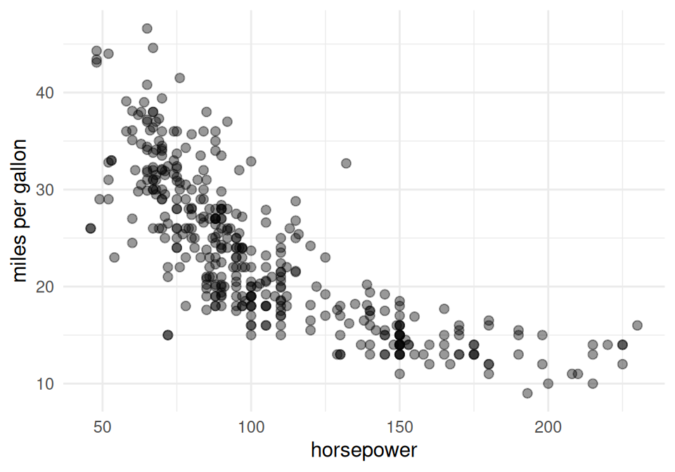
Example 19 (Correlation of horsepower and fuel economy) The Auto data record the horsepower and fuel economy (miles per gallon) of 392 car models sold between 1970 and 1982. They come from the StatLib library at Carnegie Mellon University and ship with the book An Introduction to Statistical Learning, in the Python package ISLP (ISLP.load_data("Auto")) and the R package ISLR2 (ISLR2::Auto). This site has a copy at data/auto.csv, and both code tabs below read that file.
Choose one car at random, each with the same probability, and let \(X\) be its horsepower and \(Y\) its miles per gallon. Then each expectation in the definitions of the variance and the covariance is an average over the cars in the data, and Definition 10 gives their correlation. The code below computes each part of the definition directly.
import numpy as np
import pandas as pd
auto = pd.read_csv("data/auto.csv")
x = auto["horsepower"].to_numpy(dtype=float)
y = auto["mpg"].to_numpy(dtype=float)
cov_xy = np.mean((x - x.mean()) * (y - y.mean()))
sd_x = np.sqrt(np.mean((x - x.mean()) ** 2))
sd_y = np.sqrt(np.mean((y - y.mean()) ** 2))
pd.Series({
"Cov(X, Y)": cov_xy,
"SD(X)": sd_x,
"SD(Y)": sd_y,
"Cor(X, Y)": cov_xy / (sd_x * sd_y),
})
#> Cov(X, Y) -233.261349
#> SD(X) 38.442033
#> SD(Y) 7.795046
#> Cor(X, Y) -0.778427
#> dtype: float64auto <- read.csv("data/auto.csv")
x <- auto$horsepower
y <- auto$mpg
cov_xy <- mean((x - mean(x)) * (y - mean(y)))
sd_x <- sqrt(mean((x - mean(x))^2))
sd_y <- sqrt(mean((y - mean(y))^2))
c(
"Cov(X, Y)" = cov_xy,
"SD(X)" = sd_x,
"SD(Y)" = sd_y,
"Cor(X, Y)" = cov_xy / (sd_x * sd_y)
)
#> Cov(X, Y) SD(X) SD(Y) Cor(X, Y)
#> -233.2613494 38.4420327 7.7950458 -0.7784268Figure 3 plots each car’s miles per gallon against its horsepower.
Show code
tibble::tibble(x, y) |>
ggplot2::ggplot(ggplot2::aes(x = x, y = y)) +
ggplot2::geom_point(alpha = 0.4, size = 2) +
ggplot2::labs(x = "horsepower", y = "miles per gallon") +
ggplot2::theme_minimal()The covariance is -233.3, in units of horsepower times miles per gallon. It is negative, so cars with more horsepower than average tend to have lower fuel economy than average. Dividing by the two standard deviations, 38.4 horsepower and 7.8 miles per gallon, removes the units and gives a correlation of -0.78, which lies between \(-1\) and \(1\) as Theorem 14 requires. The same value comes from R’s built-in cor(x, y), because the correlation computed from the data divides the covariance and both standard deviations by the same count, which cancels.
5MinuteAI explains variance and covariance and correlation in five minutes each, following the University of Washington’s CSE 312 [6].
6 Moments and moment generating functions
Definition 14 (Raw moment) The \(k\)-th raw moment of a random variable \(X\), for a positive integer \(k\) with \({\mathbb{E}\mathopen{}\left[\mathopen{}\left|X\right|\mathclose{}^k\right]\mathclose{}} < \infty\), is the expectation of \(X^k\):
\[{\mathbb{E}\mathopen{}\left[X^k\right]\mathclose{}}\]
Example 20 (Raw moments of a die roll) Let \(X\) be the number shown by one roll of a fair six-sided die, so that \(\mathbb{P}(X = x) = 1/6\) for each \(x \in {\mathopen{}\left\{1, 2, 3, 4, 5, 6\right\}\mathclose{}}\). The first raw moment is the expectation \({\mathbb{E}\mathopen{}\left[X\right]\mathclose{}}\), and the second is \({\mathbb{E}\mathopen{}\left[X^2\right]\mathclose{}}\):
\[ \begin{aligned} {\mathbb{E}\mathopen{}\left[X\right]\mathclose{}} &= \sum_{x=1}^{6} x \cdot\frac{1}{6} && \text{(definition of expectation)} \\ &= \frac{21}{6} && \text{(} 1 + 2 + 3 + 4 + 5 + 6 = 21 \text{)} \\ &= \frac{7}{2} && \text{(simplify)} \\ {\mathbb{E}\mathopen{}\left[X^2\right]\mathclose{}} &= \sum_{x=1}^{6} x^2 \cdot\frac{1}{6} && \text{(expectation of a function of a discrete random variable)} \\ &= \frac{91}{6} && \text{(} 1 + 4 + 9 + 16 + 25 + 36 = 91 \text{)} \end{aligned} \]
Definition 15 (Central moment) The \(k\)-th central moment of a random variable \(X\), for a positive integer \(k\) with \({\mathbb{E}\mathopen{}\left[\mathopen{}\left|X\right|\mathclose{}^k\right]\mathclose{}} < \infty\), is the expectation of the deviation from the mean raised to the power \(k\):
\[{\mathbb{E}\mathopen{}\left[[\mathbb{d}(X)]^k\right]\mathclose{}}\]
Example 21 (The third central moment of a Bernoulli random variable) Let \(X \sim \operatorname{Ber}(\pi)\), so \({\mathbb{E}\mathopen{}\left[X\right]\mathclose{}} = \pi\) and \(\mathbb{d}(X) = X - \pi\). The third central moment is:
\[ \begin{aligned} {\mathbb{E}\mathopen{}\left[[\mathbb{d}(X)]^3\right]\mathclose{}} &= \sum_{x \in {\mathopen{}\left\{0,1\right\}\mathclose{}}} (x - \pi)^3 \cdot\mathbb{P}(X = x) && \text{(expectation of a function of a discrete random variable)} \\ &= (0 - \pi)^3 (1 - \pi) + (1 - \pi)^3 \pi && \text{(substitute the Bernoulli probabilities)} \\ &= \pi(1 - \pi)\mathopen{}\left((1 - \pi)^2 - \pi^2\right)\mathclose{} && \text{(factor out } \pi(1 - \pi) \text{)} \\ &= \pi(1 - \pi)(1 - 2\pi) && \text{(difference of squares: } (1-\pi)^2 - \pi^2 = 1 - 2\pi\text{)} \end{aligned} \]
For a fair coin (\(\pi= 1/2\)), the third central moment is \(0\).
Theorem 15 (The second central moment is the variance) If \({\mathbb{E}\mathopen{}\left[X^2\right]\mathclose{}} < \infty\), then the second central moment of \(X\) is \({\operatorname{Var}\mathopen{}\left(X\right)\mathclose{}}\).
Proof. The second central moment is \({\mathbb{E}\mathopen{}\left[[\mathbb{d}(X)]^2\right]\mathclose{}}\) by Definition 15, which is \({\operatorname{Var}\mathopen{}\left(X\right)\mathclose{}}\) by Definition 3.
Example 22 (The variance of a die roll as a central moment) For the die roll \(X\) of Example 20, \({\mathbb{E}\mathopen{}\left[X\right]\mathclose{}} = 7/2\) and \({\mathbb{E}\mathopen{}\left[X^2\right]\mathclose{}} = 91/6\). By Theorem 15, the second central moment of \(X\) is the variance \({\operatorname{Var}\mathopen{}\left(X\right)\mathclose{}}\), which Theorem 2 gives as:
\[ \begin{aligned} {\operatorname{Var}\mathopen{}\left(X\right)\mathclose{}} &= {\mathbb{E}\mathopen{}\left[X^2\right]\mathclose{}} - {\mathopen{}\left({\mathbb{E}\mathopen{}\left[X\right]\mathclose{}}\right)\mathclose{}}^{2} && \text{(simplified expression for variance)} \\ &= \frac{91}{6} - \mathopen{}\left(\frac{7}{2}\right)\mathclose{}^2 && \text{(substitute the raw moments)} \\ &= \frac{182}{12} - \frac{147}{12} && \text{(common denominator)} \\ &= \frac{35}{12} && \text{(subtract)} \end{aligned} \]
Definition 16 (Moment generating function) The moment generating function of a random variable \(X\) is the function \(M_X\) of a real number \(t\) that gives the expectation of \(\text{e}^{tX}\), defined at every \(t\) with \({\mathbb{E}\mathopen{}\left[\text{e}^{tX}\right]\mathclose{}} < \infty\):
\[M_X(t) \stackrel{\text{def}}{=}{\mathbb{E}\mathopen{}\left[\text{e}^{tX}\right]\mathclose{}}\]
Example 23 (Moment generating function of a Bernoulli random variable) Let \(X \sim \operatorname{Ber}(\pi)\), so \(\mathbb{P}(X = 1) = \pi\) and \(\mathbb{P}(X = 0) = 1 - \pi\). For every \(t\):
\[ \begin{aligned} M_X(t) &= {\mathbb{E}\mathopen{}\left[\text{e}^{tX}\right]\mathclose{}} && \text{(definition of the moment generating function)} \\ &= \sum_{x \in {\mathopen{}\left\{0,1\right\}\mathclose{}}} \text{e}^{tx} \cdot\mathbb{P}(X = x) && \text{(expectation of a function of a discrete random variable)} \\ &= \text{e}^{0} \cdot(1 - \pi) + \text{e}^{t} \cdot\pi && \text{(substitute the Bernoulli probabilities)} \\ &= 1 - \pi+ \pi\,\text{e}^{t} && \text{(} \text{e}^{0} = 1 \text{)} \end{aligned} \]
Theorem 16 (Moments from the moment generating function) If \(M_X(t)\) is defined at every \(t\) in some open interval around \(0\), then for every positive integer \(k\), the \(k\)-th raw moment of \(X\) is the \(k\)-th derivative of \(M_X\) at \(0\):
\[{\mathbb{E}\mathopen{}\left[X^k\right]\mathclose{}} = M_X^{(k)}(0)\]
Proof. Let \(h > 0\) be such that \(M_X(t)\) is defined for every \(\mathopen{}\left|t\right|\mathclose{} < h\). For any such \(t\), the series of the exponential gives:
\[\text{e}^{tX} = \sum_{k=0}^{\infty} \frac{t^k X^k}{k!}\]
The absolute value of each summand is at most the matching summand of \(\text{e}^{\mathopen{}\left|tX\right|\mathclose{}}\). Also, \(\text{e}^{\mathopen{}\left|tX\right|\mathclose{}} \le \text{e}^{tX} + \text{e}^{-tX}\), and \(M_X(t)\) and \(M_X(-t)\) are both defined, so \({\mathbb{E}\mathopen{}\left[\text{e}^{\mathopen{}\left|tX\right|\mathclose{}}\right]\mathclose{}} < \infty\). This domination lets the expectation pass through the series, by the Fubini–Tonelli exchange:
\[ \begin{aligned} M_X(t) &= {\mathbb{E}\mathopen{}\left[\sum_{k=0}^{\infty} \frac{t^k X^k}{k!}\right]\mathclose{}} && \text{(power series of the exponential)} \\ &= \sum_{k=0}^{\infty} \frac{t^k}{k!}{\mathbb{E}\mathopen{}\left[X^k\right]\mathclose{}} && \text{(pass the expectation through the sum; linearity of expectation)} \end{aligned} \]
A Taylor series can be differentiated one summand at a time inside the open interval where it converges. The \(k\)-th derivative at \(0\) keeps only the summand with \(t^k\), and that summand’s coefficient is multiplied by \(k!\). So \(M_X^{(k)}(0) = k! \cdot\frac{{\mathbb{E}\mathopen{}\left[X^k\right]\mathclose{}}}{k!} = {\mathbb{E}\mathopen{}\left[X^k\right]\mathclose{}}\).
Example 24 (Moments of a Bernoulli random variable from its moment generating function) For \(X \sim \operatorname{Ber}(\pi)\), Example 23 gives \(M_X(t) = 1 - \pi+ \pi\,\text{e}^{t}\) for every \(t\), so \(M_X^{(k)}(t) = \pi\,\text{e}^{t}\) for every \(k \ge 1\). By Theorem 16, for every \(k \ge 1\):
\[ \begin{aligned} {\mathbb{E}\mathopen{}\left[X^k\right]\mathclose{}} &= M_X^{(k)}(0) && \text{(moments from the moment generating function)} \\ &= \pi\,\text{e}^{0} && \text{(} M_X^{(k)}(t) = \pi\,\text{e}^{t} \text{)} \\ &= \pi && \text{(} \text{e}^{0} = 1 \text{)} \end{aligned} \]
This agrees with the direct computation of \({\mathbb{E}\mathopen{}\left[X^2\right]\mathclose{}}\) for a Bernoulli variable on the expectation page.
Theorem 17 (Moment generating function of a sum of independent random variables) If \(X\) and \(Y\) are independent, and \(M_X(t)\) and \(M_Y(t)\) are defined at a number \(t\), then:
\[M_{X+Y}(t) = M_X(t)\,M_Y(t)\]
Proof. Functions of independent variables are independent, so \(\text{e}^{tX}\) and \(\text{e}^{tY}\) are independent. Independent variables \(A\) and \(B\) satisfy \({\mathbb{E}\mathopen{}\left[AB\right]\mathclose{}} = {\mathbb{E}\mathopen{}\left[A\right]\mathclose{}}\,{\mathbb{E}\mathopen{}\left[B\right]\mathclose{}}\), so:
\[ \begin{aligned} M_{X+Y}(t) &= {\mathbb{E}\mathopen{}\left[\text{e}^{t(X+Y)}\right]\mathclose{}} && \text{(definition of the moment generating function)} \\ &= {\mathbb{E}\mathopen{}\left[\text{e}^{tX}\,\text{e}^{tY}\right]\mathclose{}} && \text{(} \text{e}^{a+b} = \text{e}^{a}\,\text{e}^{b} \text{)} \\ &= {\mathbb{E}\mathopen{}\left[\text{e}^{tX}\right]\mathclose{}}\,{\mathbb{E}\mathopen{}\left[\text{e}^{tY}\right]\mathclose{}} && \text{(expectation of a product of independent variables)} \\ &= M_X(t)\,M_Y(t) && \text{(definition of the moment generating function)} \end{aligned} \]
Example 25 (Moment generating function of a binomial random variable) By the sum of Bernoulli variables, a binomial random variable \(S \sim {\operatorname{Bin}\mathopen{}\left(n, \pi\right)\mathclose{}}\) is a sum \(S = \sum_{i=1}^n X_i\) of \(n\) independent \(\operatorname{Ber}(\pi)\) variables. Each has moment generating function \(1 - \pi+ \pi\,\text{e}^{t}\) (Example 23). Applying Theorem 17 one summand at a time:
\[ \begin{aligned} M_S(t) &= \prod_{i=1}^{n} M_{X_i}(t) && \text{(moment generating function of a sum of independent random variables)} \\ &= \mathopen{}\left(1 - \pi+ \pi\,\text{e}^{t}\right)\mathclose{}^n && \text{(each factor is the Bernoulli moment generating function)} \end{aligned} \]
Definitions on this page
- Definition 1 (Deviation)
- Definition 2 (Deviation from a population or subpopulation mean (error, noise term))
- Definition 3 (Variance)
- Definition 4 (Conditional variance)
- Definition 5 (Homoskedasticity)
- Definition 6 (Heteroskedasticity)
- Definition 7 (Precision)
- Definition 8 (Standard deviation)
- Definition 9 (Covariance)
- Definition 10 (Correlation)
- Definition 11 (Uncorrelated random variables)
- Definition 12 (Conditional covariance)
- Definition 13 (Variance/covariance of a \(p \times 1\) random vector)
- Definition 14 (Raw moment)
- Definition 15 (Central moment)
- Definition 16 (Moment generating function)