Last modified: 2026-11-19
Source
The first section and the definition of a decision boundary moved here from Logistic Regression, whose Source note lists that page’s sources. The definition of a decision region moved here from Support Vector Machines.
Linear regression predicts a number. A great many questions are not about a number: whether a patient recovers, whether an email is spam, which of ten digits a scan shows.
Let the data be \(\mathcal{X} = \set{(\vx_1, y_1), \ldots, (\vx_n, y_n)}\) with \(\vx_i \in \reals^{\ninputvars}\) and \(y_i\) a label rather than a measurement. Two labels is binary classification; more than two is multi-class classification.
We could predict the label directly, with a classification rule that maps each feature vector to one of the classes. Predicting \(\Prf{Y = 1 \mid \vx}\) gives more information. A predicted class label names only a class; a predicted probability also measures how likely each class is, so whoever uses the prediction can choose how to act on it, for instance with a threshold that reflects the cost of each kind of error.
Watch
Hutchinson teaches classification and decision boundaries (6 min) [1]. The video site requires a login, which enrolled students find in the syllabus.
A classification rule splits the set of all feature vectors into pieces, one for each class that it predicts.
Definition 1 (Decision region)
Definition 1 (Decision region) The decision region of a class \(k\) under a classification rule \(c\) is the set of feature vectors that \(c\) assigns to \(k\):
\[ \setbuild{\vx}{c(\vx) = k}. \]
Example 1 (Decision regions of a blood-pressure rule)
Example 1 (Decision regions of a blood-pressure rule) A cohort study, the Western Collaborative Group Study [2], followed 3154 middle-aged men for coronary heart disease, and recorded each man’s systolic blood pressure \(\predvar\), in mmHg. Let the classification rule \(c\) predict heart disease (\(c(\predvar) = 1\)) when \(\predvar \ge 140\), and no heart disease (\(c(\predvar) = 0\)) otherwise. We chose the cutoff 140 mmHg by hand, as a round number in the upper part of the data; logistic regression instead fits a classifier to data. The decision region of class \(1\) is \(\setbuild{\predvar}{\predvar \ge 140}\), and the decision region of class \(0\) is \(\setbuild{\predvar}{\predvar < 140}\). 693 of the men are in the first region, and 2461 are in the second. Figure 1 shades the two regions over the men’s blood pressures, with one bar for each recorded pressure.
outcome_levels <- c("No heart disease", "Heart disease")
outcome <- ifelse(wcgs$chd == 1, "Heart disease", "No heart disease")
wcgs$outcome <- factor(outcome, outcome_levels)
sbp_range <- range(wcgs$sbp)
region_names <- c("Predicted no heart disease", "Predicted heart disease")
region_starts <- c(sbp_range[1] - 1, sbp_cutoff)
region_ends <- c(sbp_cutoff, sbp_range[2] + 1)
regions <- tibble::tibble(
xmin = region_starts,
xmax = region_ends,
region = region_names
)
region_fill <- c(
"Predicted no heart disease" = "#56B4E9",
"Predicted heart disease" = "#E69F00"
)
region_aes <- ggplot2::aes(
xmin = xmin, xmax = xmax, ymin = -Inf, ymax = Inf, fill = region
)
panels <- ggplot2::vars(outcome)
wcgs |>
ggplot2::ggplot() +
ggplot2::aes(x = sbp) +
ggplot2::geom_rect(
region_aes,
data = regions,
inherit.aes = FALSE,
alpha = 0.3
) +
ggplot2::geom_bar() +
ggplot2::geom_vline(xintercept = sbp_cutoff, linetype = "dashed") +
ggplot2::facet_wrap(panels, ncol = 1, scales = "free_y") +
ggplot2::scale_fill_manual(values = region_fill) +
ggplot2::labs(
x = "Systolic blood pressure (mmHg)",
y = "Number of men",
fill = "Decision region"
)Example 2 (The men who had heart disease are not a decision region)
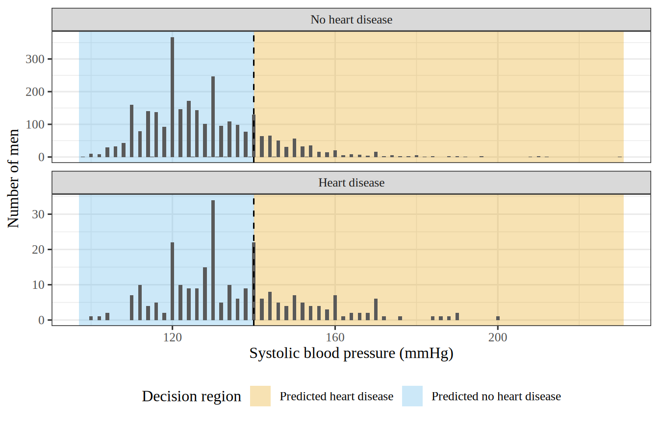
Example 2 (The men who had heart disease are not a decision region) In the Western Collaborative Group Study data of Example 1, 257 men had coronary heart disease. The set of their blood pressures is not the decision region of class \(1\) under the rule \(c\) of Example 1, because a decision region depends on what \(c\) predicts, not on the observed labels. Only 96 of those men are in the decision region of class \(1\); the other 161 had blood pressures below 140 mmHg, so \(c\) predicts no heart disease for them.
Definition 2 (Decision boundary)
Definition 2 (Decision boundary) The decision boundary of a classifier is the set of feature vectors that separates the decision regions where it predicts different classes.
Example 3 (Decision boundary of a blood-pressure rule)
Example 3 (Decision boundary of a blood-pressure rule) The rule \(c\) of Example 1 predicts heart disease when the systolic blood pressure \(\predvar\) is at least 140 mmHg. Its decision boundary is the single point \(\predvar = 140\), which lies between the decision region \(\setbuild{\predvar}{\predvar < 140}\) and the decision region \(\setbuild{\predvar}{\predvar \ge 140}\). It is the dashed line in Figure 1.
Example 4 (A cutoff that is not a decision boundary)
Example 4 (A cutoff that is not a decision boundary) The point \(\predvar = 120\) is not on the decision boundary of the rule \(c\) of Example 1. Blood pressures slightly below and slightly above 120 mmHg are both in the decision region of class \(0\), so the point does not separate two decision regions.
The error rate of a classification rule counts how often it misclassifies. Example 5 and Example 6 compute it for two rules on the men of the Western Collaborative Group Study.
Example 5 (Error rate of a blood-pressure rule)
Example 5 (Error rate of a blood-pressure rule) The rule \(c\) of Example 1 makes two kinds of mistake on the 3154 men. It predicts heart disease for 597 men who had none, and predicts no heart disease for 161 men who had it. Its error rate on these men is therefore
\[ \frac{758}{3154} \approx 0.240. \]
Example 6 (A rule that never predicts heart disease)
Example 6 (A rule that never predicts heart disease) A second rule \(c_0\) predicts no heart disease for every man, so \(c_0(\predvar) = 0\) whatever \(\predvar\) is. It is wrong only for the 257 men who had heart disease, so its error rate on the 3154 men is
\[ \frac{257}{3154} \approx 0.081. \]
This error rate is lower than that of the rule \(c\) in Example 5, even though \(c_0\) never finds a single case of heart disease. Heart disease is rare in these data, so the error rate alone favors a rule that ignores blood pressure. The Metrics page reports each kind of mistake separately.
Logistic Regression fits a classifier to data, instead of choosing its cutoff by hand. The Metrics page reports how often a classifier’s predictions are wrong.