Key distributions

Published

Last modified: 2026-11-13 06:54:40 (PST)

Remark

Remark. Some distributions are typically used for outcome models (Table 1); other distributions are typically used for test statistics (Table 2).

Table 1: Distributions typically used for outcome models

Distribution	Uses
Bernoulli	Binary outcomes
Binomial	Sums of Bernoulli outcomes
Poisson	Unbounded count outcomes
Geometric	Counts of non-events before an event occurs
Negative binomial	Mixtures of Poisson distributions, counts of non-events until a given number of events occurs
Normal (Gaussian)	Continuous outcomes without a more specific distribution
Multivariate normal	Vectors of continuous outcomes
Mixtures	Outcomes from a population of unobserved subpopulations
Exponential	Time to event outcomes
Gamma	Time to event outcomes
Weibull	Time to event outcomes
Log-normal	Time to event outcomes

Table 2: Distributions typically used for test statistics

Distribution	Uses
$\chi^2$	Regression comparisons (asymptotic), contingency table independence tests, goodness-of-fit tests
$F$	Gaussian model comparisons (exact)
$Z$ (standard normal)	Proportions, means, regression coefficients (asymptotic)
$t$ (Student’s)	Means, regression coefficients in Gaussian outcome models (exact)

1 The Bernoulli distribution

Example 1 (A coin flip)

Example 1 (A coin flip) The Bernoulli distribution describes a binary outcome. The indicator of heads on one flip of a fair coin is $\operatorname{Ber}(1/2)$. By the expectation of the Bernoulli distribution, $X \sim \operatorname{Ber}(\pi)$ has mean $\pi$, and by the variance of a Bernoulli random variable, it has variance $\pi(1 - \pi)$.

2 The binomial distribution

Definition 1 (Binomial distribution)

Definition 1 (Binomial distribution) A discrete random variable $X$ has the binomial distribution with number of trials $n \in {\mathopen{}\left\{1, 2, \dots\right\}\mathclose{}}$ and event probability $\pi\in [0, 1]$, written $X \sim {\operatorname{Bin}\mathopen{}\left(n, \pi\right)\mathclose{}}$ [1], if:

\[ \mathbb{P}(X = x) \stackrel{\text{def}}{=}\binom{n}{x} \pi^x (1 - \pi)^{n - x}, \quad x \in {\mathopen{}\left\{0, 1, \dots, n\right\}\mathclose{}} \tag{1}\]

where $\binom{n}{x} = \frac{n!}{x!\,(n - x)!}$ is the number of ways to choose $x$ of the $n$ trials.

Remark

Remark. Casella and Berger [2, Sec. 3.2] defines the binomial distribution the same way. With $n = 1$, Equation 1 is the Bernoulli PMF: ${\operatorname{Bin}\mathopen{}\left(1, \pi\right)\mathclose{}}$ and $\operatorname{Ber}(\pi)$ are the same distribution.

Example 2 (Two heads in three flips)

Example 2 (Two heads in three flips) Let $X \sim {\operatorname{Bin}\mathopen{}\left(3, 1/2\right)\mathclose{}}$ be the number of heads in three flips of a fair coin. By Equation 1:

\[ \begin{aligned} \mathbb{P}(X = 2) &= \binom{3}{2} \mathopen{}\left(\frac{1}{2}\right)\mathclose{}^2 \mathopen{}\left(1 - \frac{1}{2}\right)\mathclose{}^{3 - 2} && \text{(binomial PMF with } n = 3,\ \pi= 1/2,\ x = 2 \text{)} \\ &= \frac{3!}{2!\,1!} \mathopen{}\left(\frac{1}{2}\right)\mathclose{}^2 \mathopen{}\left(\frac{1}{2}\right)\mathclose{}^1 && \text{(definition of } \tbinom{3}{2} \text{; } 1 - 1/2 = 1/2 \text{)} \\ &= 3 \cdot\frac{1}{4} \cdot\frac{1}{2} && \text{(evaluate the factorials and powers)} \\ &= \frac{3}{8} && \text{(multiply)} \end{aligned} \]

The three outcomes with two heads are $HHT$, $HTH$, and $THH$, each with probability $1/8$.

Example 3 (Draws without replacement are not binomial)

Example 3 (Draws without replacement are not binomial) An urn holds two red balls and two blue balls. Draw two balls without replacement, and let $X$ be the number of red balls drawn. Each draw is red with probability $1/2$, but $X \not\sim {\operatorname{Bin}\mathopen{}\left(2, 1/2\right)\mathclose{}}$, because the draws are not independent:

\[ \begin{aligned} \mathbb{P}(X = 2) &= \mathbb{P}(\text{first red}) \cdot\mathbb{P}(\text{second red} \mid \text{first red}) && \text{(multiplication rule)} \\ &= \frac{2}{4} \cdot\frac{1}{3} && \text{(one red ball is left among three)} \\ &= \frac{1}{6} && \text{(multiply)} \end{aligned} \]

whereas, by Equation 1, a ${\operatorname{Bin}\mathopen{}\left(2, 1/2\right)\mathclose{}}$ random variable has

\[ \begin{aligned} \mathbb{P}(X = 2) &= \binom{2}{2} \mathopen{}\left(\frac{1}{2}\right)\mathclose{}^2 \mathopen{}\left(\frac{1}{2}\right)\mathclose{}^0 && \text{(binomial PMF with } n = 2,\ \pi= 1/2,\ x = 2 \text{)} \\ &= \frac{1}{4} && \text{(evaluate)} \end{aligned} \]

Theorem 1 (A sum of IID Bernoulli variables is binomial)

Theorem 1 (A sum of IID Bernoulli variables is binomial) If $X_1, \ldots, X_n$ are IID $\operatorname{Ber}(\pi)$ random variables, then their sum $S = \sum_{i=1}^nX_i$ has the ${\operatorname{Bin}\mathopen{}\left(n, \pi\right)\mathclose{}}$ distribution.

Proof

Proof. Each $X_i$ is $0$ or $1$, so $S$ takes values in ${\mathopen{}\left\{0, 1, \dots, n\right\}\mathclose{}}$. Let $x \in {\mathopen{}\left\{0, 1, \dots, n\right\}\mathclose{}}$ be a value of $S$, and let $A_x$ be the set of sequences $(s_1, \ldots, s_n) \in {\mathopen{}\left\{0, 1\right\}\mathclose{}}^n$ with exactly $x$ ones. The event ${\mathopen{}\left\{S = x\right\}\mathclose{}}$ is the disjoint union of the events ${\mathopen{}\left\{X_1 = s_1, \ldots, X_n = s_n\right\}\mathclose{}}$ over $(s_1, \ldots, s_n) \in A_x$. For one such sequence:

\[ \begin{aligned} \mathbb{P}(X_1 = s_1, \ldots, X_n = s_n) &= \prod_{i=1}^n \mathbb{P}(X_i = s_i) && \text{(independence)} \\ &= \prod_{i=1}^n \pi^{s_i} (1 - \pi)^{1 - s_i} && \text{(Bernoulli PMF)} \\ &= \pi^{\sum_{i=1}^ns_i} (1 - \pi)^{\sum_{i=1}^n(1 - s_i)} && \text{(collect exponents)} \\ &= \pi^x (1 - \pi)^{n - x} && \text{(} \textstyle\sum_{i=1}^ns_i = x \text{ for a sequence in } A_x \text{)} \end{aligned} \]

Choosing which $x$ of the $n$ positions hold the ones determines the sequence, so $A_x$ has $\binom{n}{x}$ elements. Therefore:

\[ \begin{aligned} \mathbb{P}(S = x) &= \sum_{(s_1, \ldots, s_n) \in A_x} \mathbb{P}(X_1 = s_1, \ldots, X_n = s_n) && \text{(additivity over disjoint events)} \\ &= \sum_{(s_1, \ldots, s_n) \in A_x} \pi^x (1 - \pi)^{n - x} && \text{(probability of one sequence)} \\ &= \binom{n}{x} \pi^x (1 - \pi)^{n - x} && \text{(} A_x \text{ has } \tbinom{n}{x} \text{ elements)} \end{aligned} \]

which is Equation 1.

Example 4 (Counting treatment responders)

Example 4 (Counting treatment responders) Suppose five patients each respond to a treatment with probability $0.2$, independently of one another, and let $X_i = 1$ if patient $i$ responds and $X_i = 0$ otherwise. By Theorem 1, the number of responders $S = \sum_{i=1}^5 X_i$ is ${\operatorname{Bin}\mathopen{}\left(5, 0.2\right)\mathclose{}}$, so the probability that nobody responds is:

\[ \begin{aligned} \mathbb{P}(S = 0) &= \binom{5}{0} (0.2)^0 (1 - 0.2)^{5 - 0} && \text{(binomial PMF with } n = 5,\ \pi= 0.2,\ x = 0 \text{)} \\ &= 1 \cdot 1 \cdot(0.8)^5 && \text{(} \tbinom{5}{0} = 1 \text{ and } (0.2)^0 = 1 \text{)} \\ &= 0.32768 && \text{(evaluate the power)} \end{aligned} \]

Theorem 2 (Mean and variance of the binomial distribution)

Theorem 2 (Mean and variance of the binomial distribution) If $X \sim {\operatorname{Bin}\mathopen{}\left(n, \pi\right)\mathclose{}}$, then:

${\mathbb{E}\mathopen{}\left[X\right]\mathclose{}} = n\pi$
${\operatorname{Var}\mathopen{}\left(X\right)\mathclose{}} = n\pi(1 - \pi)$

Proof

Proof. The mean and variance of $X$ depend only on its distribution, so by Theorem 1 we can compute them for $S = \sum_{i=1}^nX_i$, where $X_1, \ldots, X_n$ are IID $\operatorname{Ber}(\pi)$. For the mean, apply linearity of expectation $n - 1$ times, then the Bernoulli mean:

\[ \begin{aligned} {\mathbb{E}\mathopen{}\left[S\right]\mathclose{}} &= {\mathbb{E}\mathopen{}\left[\sum_{i=1}^nX_i\right]\mathclose{}} && \text{(definition of } S \text{)} \\ &= \sum_{i=1}^n{\mathbb{E}\mathopen{}\left[X_i\right]\mathclose{}} && \text{(linearity of expectation)} \\ &= \sum_{i=1}^n\pi && \text{(Bernoulli mean)} \\ &= n\pi && \text{(sum of } n \text{ copies of } \pi\text{)} \end{aligned} \]

For the variance, apply the variance of a linear combination with $a_1 = \cdots = a_n = 1$, then independent components give a diagonal variance matrix, then the Bernoulli variance:

\[ \begin{aligned} {\operatorname{Var}\mathopen{}\left(S\right)\mathclose{}} &= \sum_{i=1}^n\sum_{j=1}^n {\operatorname{Cov}\mathopen{}\left(X_i, X_j\right)\mathclose{}} && \text{(variance of a linear combination with } a_i = 1 \text{)} \\ &= \sum_{i=1}^n{\operatorname{Cov}\mathopen{}\left(X_i, X_i\right)\mathclose{}} && \text{(} {\operatorname{Cov}\mathopen{}\left(X_i, X_j\right)\mathclose{}} = 0 \text{ for } i \neq j \text{, by independence)} \\ &= \sum_{i=1}^n{\operatorname{Var}\mathopen{}\left(X_i\right)\mathclose{}} && \text{(} {\operatorname{Cov}\mathopen{}\left(X_i, X_i\right)\mathclose{}} = {\operatorname{Var}\mathopen{}\left(X_i\right)\mathclose{}} \text{)} \\ &= \sum_{i=1}^n\pi(1 - \pi) && \text{(Bernoulli variance)} \\ &= n\pi(1 - \pi) && \text{(sum of } n \text{ copies of } \pi(1 - \pi) \text{)} \end{aligned} \]

Example 5 (Expected number of responders)

Example 5 (Expected number of responders) In Example 4, $S \sim {\operatorname{Bin}\mathopen{}\left(5, 0.2\right)\mathclose{}}$. By Theorem 2:

\[ \begin{aligned} {\mathbb{E}\mathopen{}\left[S\right]\mathclose{}} &= 5 \cdot 0.2 && \text{(} n\pi\text{)} \\ &= 1 && \text{(multiply)} \\ {\operatorname{Var}\mathopen{}\left(S\right)\mathclose{}} &= 5 \cdot 0.2 \cdot(1 - 0.2) && \text{(} n\pi(1 - \pi) \text{)} \\ &= 0.8 && \text{(multiply)} \end{aligned} \]

On average, one of the five patients responds.

3 The Poisson distribution

Definition 2 (Poisson distribution)

Definition 2 (Poisson distribution) A random variable $Y$ has the Poisson distribution with mean parameter $\mu> 0$, written $Y \sim \operatorname{Pois}(\mu)$ [3], if:

\[\mathbb{P}(Y = y) \stackrel{\text{def}}{=}\frac{\mu^{y} \text{e}^{-\mu}}{y!} \, \text{1}_{y \in \mathbb{N}}, \quad y \in \mathbb{R} \tag{2}\]

where $\mathbb{N}= {\mathopen{}\left\{0, 1, 2, \dots\right\}\mathclose{}}$ is the set of non-negative integers. The indicator makes the mass $0$ outside $\mathbb{N}$, where $y!$ is undefined.

Remark

Remark. (see Figure 1)

Exercise 1

Exercise 1 What is the range of possible values for a Poisson distribution?

Solution 1

Solution 1. \[ \begin{aligned} \mathcal{R}(Y) &= {\mathopen{}\left\{0, 1, 2, \dots\right\}\mathclose{}} \\ &= \mathbb{N} \end{aligned} \]

Theorem 3 (CDF of Poisson distribution)

Theorem 3 (CDF of Poisson distribution) If $Y \sim \operatorname{Pois}(\mu)$, then for every real number $y$:

\[\mathbb{P}(Y \le y) = e^{-\mu} \sum_{j=0}^{\mathopen{}\left\lfloor y\right\rfloor\mathclose{}}\frac{\mu^j}{j!} \tag{3}\]

Proof

Proof. For $y < 0$, both sides are $0$ (the sum is empty). For any $y \ge 0$, the event $\{Y \le y\}$ is the disjoint union of events $\{Y = j\}$ for all non-negative integers $j \le \mathopen{}\left\lfloor y\right\rfloor\mathclose{}$. Applying the Poisson PMF (Equation 2) and factoring out the common term $e^{-\mu}$:

\[ \begin{aligned} \mathbb{P}(Y \le y) &= \sum_{j=0}^{\mathopen{}\left\lfloor y\right\rfloor\mathclose{}} \mathbb{P}(Y = j) && (\text{disjoint union of events } Y = j) \\ &= \sum_{j=0}^{\mathopen{}\left\lfloor y\right\rfloor\mathclose{}} \frac{\mu^j e^{-\mu}}{j!} && (\text{definition of Poisson PMF}) \\ &= e^{-\mu} \sum_{j=0}^{\mathopen{}\left\lfloor y\right\rfloor\mathclose{}} \frac{\mu^j}{j!} && (\text{factoring out } e^{-\mu} \text{ constant wrt } j) \end{aligned} \]

Example 6 (Computing Poisson cumulative probabilities)

Example 6 (Computing Poisson cumulative probabilities) For a Poisson random variable $X \sim \operatorname{Pois}(\mu= 2)$, the probability of observing at most 2 events is computed as:

\[ \begin{aligned} \mathbb{P}(X \le 2) &= e^{-2} \sum_{j=0}^{2} \frac{2^j}{j!} && (\text{apply CDF formula with } \mu= 2, y = 2) \\ &= e^{-2} \mathopen{}\left(\frac{2^0}{0!} + \frac{2^1}{1!} + \frac{2^2}{2!}\right)\mathclose{} && (\text{expand terms for } j = 0, 1, 2) \\ &= e^{-2} \mathopen{}\left(1 + 2 + 2\right)\mathclose{} && (\text{simplify factorials and powers}) \\ &= 5 e^{-2} \approx 0.677 && (\text{evaluate numerical value}) \end{aligned} \]

Remark

Remark. (see Figure 2)

Show code

pois_dists <-
  dplyr::tibble(mu = c(0.5, 1, 2, 5, 10, 20)) |>
  dplyr::reframe(.by = mu, x = 0:30) |>
  dplyr::mutate(
    `P(X = x)` = dpois(x, lambda = mu),
    `P(X <= x)` = ppois(x, lambda = mu),
    mu = factor(mu)
  )

plot0 <-
  pois_dists |>
  ggplot2::ggplot(
    ggplot2::aes(
      x = x,
      y = `P(X = x)`,
      fill = mu,
      col = mu
    )
  ) +
  ggplot2::theme(legend.position = "bottom") +
  ggplot2::labs(
    fill = latex2exp::TeX("$\\mu$"),
    col = latex2exp::TeX("$\\mu$"),
    y = latex2exp::TeX("$\\Pr_{\\mu}(X = x)$")
  )

plot1 <-
  plot0 +
  ggplot2::geom_segment(yend = 0) +
  ggplot2::facet_wrap(~mu)

print(plot1)

Figure 1: Poisson PMFs, by mean parameter $\mu$

Show code

plot2 <-
  plot0 +
  ggplot2::geom_step(alpha = 0.75) +
  ggplot2::aes(y = `P(X <= x)`) +
  ggplot2::labs(y = latex2exp::TeX("$\\Pr_{\\mu}(X \\leq x)$"))

print(plot2)

Exercise 2 (Poisson distribution functions)

Exercise 2 (Poisson distribution functions) Let $X \sim \operatorname{Pois}(\mu= 3.75)$.

Compute:

$\mathbb{P}(X = 4)$
$\mathbb{P}(X \le 7)$
$\mathbb{P}(X > 5)$

Solution

Solution.

$\mathbb{P}(X=4) = 0.1937803$
$\mathbb{P}(X\le 7) = 0.9623787$
$\mathbb{P}(X > 5) = 0.1771172$

Theorem 4 (Mean and variance of the Poisson distribution)

Theorem 4 (Mean and variance of the Poisson distribution) If $X \sim \operatorname{Pois}(\mu)$, then:

$\mathbb{E}[X] = \mu$
$\operatorname{Var}(X) = \mu$

Proof

Proof. Mean.

\[ \begin{aligned} \mathbb{E}[X] &= \sum_{x=0}^\infty x \cdot \mathbb{P}(X=x) && (\text{definition of expected value}) \\ &= 0 \cdot \mathbb{P}(X=0) + \sum_{x=1}^{\infty} x \cdot \mathbb{P}(X=x) && (\text{separate } x=0 \text{ term}) \\ &= \sum_{x=1}^{\infty} x \cdot \frac{\mu^x e^{-\mu}}{x!} && (\text{substitute Poisson PMF}) \\ &= \sum_{x=1}^{\infty} x \cdot \frac{\mu^x e^{-\mu}}{x \cdot (x-1)!} && (\text{definition of factorial } x!) \\ &= \sum_{x=1}^{\infty} \frac{\mu^x e^{-\mu}}{(x-1)!} && (\text{cancel factor of } x) \\ &= \mu\cdot \sum_{x=1}^{\infty} \frac{\mu^{x-1} e^{-\mu}}{(x-1)!} && (\text{factor out one power of } \mu) \\ &= \mu\cdot \sum_{y=0}^\infty \frac{\mu^y e^{-\mu}}{y!} && (\text{change index variable } y \stackrel{\text{def}}{=}x-1) \\ &= \mu\cdot 1 && (\text{PMF sums to 1 over state space}) \\ &= \mu&& (\text{simplify}) \end{aligned} \]

Variance. The same steps, canceling two factors instead of one, give ${\mathbb{E}\mathopen{}\left[X(X-1)\right]\mathclose{}}$:

\[ \begin{aligned} {\mathbb{E}\mathopen{}\left[X(X-1)\right]\mathclose{}} &= \sum_{x=2}^\infty x(x-1) \cdot \frac{\mu^x e^{-\mu}}{x!} && (\text{LOTUS; the } x = 0, 1 \text{ terms are } 0) \\ &= \sum_{x=2}^\infty \frac{\mu^x e^{-\mu}}{(x-2)!} && (\text{cancel } x(x-1) \text{ against } x!) \\ &= \mu^2 \cdot \sum_{y=0}^\infty \frac{\mu^y e^{-\mu}}{y!} && (\text{factor out } \mu^2 \text{; } y \stackrel{\text{def}}{=}x - 2) \\ &= \mu^2 && (\text{PMF sums to 1}) \end{aligned} \]

Then, by the simplified expression for variance and linearity of expectation:

\[ \begin{aligned} \operatorname{Var}(X) &= {\mathbb{E}\mathopen{}\left[X^2\right]\mathclose{}} - {\mathopen{}\left({\mathbb{E}\mathopen{}\left[X\right]\mathclose{}}\right)\mathclose{}}^{2} && (\text{simplified expression for variance}) \\ &= {\mathbb{E}\mathopen{}\left[X(X-1)\right]\mathclose{}} + {\mathbb{E}\mathopen{}\left[X\right]\mathclose{}} - {\mathopen{}\left({\mathbb{E}\mathopen{}\left[X\right]\mathclose{}}\right)\mathclose{}}^{2} && (X^2 = X(X-1) + X \text{; linearity}) \\ &= \mu^2 + \mu- \mu^2 && (\text{substitute}) \\ &= \mu&& (\text{simplify}) \end{aligned} \]

Theorem 5 (Ratio of consecutive Poisson probabilities, and the mode)

Theorem 5 (Ratio of consecutive Poisson probabilities, and the mode) If $X \sim \operatorname{Pois}(\mu)$, then:

$\mathbb{P}(X=x) = \frac{\mu}{x} \mathbb{P}(X = x-1)$ for $x \in {\mathopen{}\left\{1, 2, \dots\right\}\mathclose{}}$
For $x \in {\mathopen{}\left\{1, 2, \dots\right\}\mathclose{}}$ with $x < \mu$, $\mathbb{P}(X=x) > \mathbb{P}(X = x-1)$
For $x = \mu$ (possible only when $\mu$ is an integer), $\mathbb{P}(X=x) = \mathbb{P}(X = x-1)$
For $x \in {\mathopen{}\left\{1, 2, \dots\right\}\mathclose{}}$ with $x > \mu$, $\mathbb{P}(X=x) < \mathbb{P}(X = x-1)$
If $\mu$ is not an integer, $\arg \max_{x} \mathbb{P}(X=x) = \mathopen{}\left\lfloor\mu\right\rfloor\mathclose{}$; if $\mu$ is an integer, the maximum is attained at both $x = \mu- 1$ and $x = \mu$

Proof

Proof. Ratio of consecutive probabilities. For $x \in {\mathopen{}\left\{1, 2, \dots\right\}\mathclose{}}$:

\[ \begin{aligned} \frac{\mathbb{P}(X = x)}{\mathbb{P}(X = x - 1)} &= \frac{\mu^x e^{-\mu} / x!}{\mu^{x-1} e^{-\mu} / (x-1)!} && (\text{substitute Poisson PMF}) \\ &= \frac{\mu}{x} && (\text{cancel } \mu^{x-1} e^{-\mu} \text{ and } (x-1)!) \end{aligned} \]

This ratio is greater than, equal to, or less than 1 as $x$ is less than, equal to, or greater than $\mu$, which gives the three comparisons. So $\mathbb{P}(X = x)$ increases while $x < \mu$ and decreases once $x > \mu$. If $\mu$ is not an integer, the last increase is at $x = \mathopen{}\left\lfloor\mu\right\rfloor\mathclose{}$, which is therefore the unique mode. If $\mu$ is an integer, $\mathbb{P}(X = \mu) = \mathbb{P}(X = \mu- 1)$, and both are modes.

Example 7 (Mode of a Poisson distribution)

Example 7 (Mode of a Poisson distribution) For $X \sim \operatorname{Pois}(2.5)$, $\mathbb{P}(X = 2) = \frac{2.5}{2}\mathbb{P}(X = 1) > \mathbb{P}(X = 1)$ and $\mathbb{P}(X = 3) = \frac{2.5}{3}\mathbb{P}(X = 2) < \mathbb{P}(X = 2)$, so the mode is $\mathopen{}\left\lfloor 2.5\right\rfloor\mathclose{} = 2$. For $X \sim \operatorname{Pois}(2)$, $\mathbb{P}(X = 2) = \frac{2}{2}\mathbb{P}(X = 1)$, so $1$ and $2$ are both modes, each with probability $2 e^{-2} \approx 0.271$.

Definition 3 (Exposure magnitude)

Definition 3 (Exposure magnitude) For many count outcomes, there is some sense of an exposure magnitude, such as population size or duration of observation, which multiplicatively rescales the expected (mean) count.

Exercise 3

Exercise 3 What are some examples of exposure magnitudes?

Solution

Solution.

Table 3: Examples of exposure units

outcome	exposure units
disease incidence	number of individuals exposed; time at risk
car accidents	miles driven
worksite accidents	person-hours worked
population size	size of habitat

Remark

Remark. Exposure units are similar to the number of trials in a binomial distribution, but in non-binomial count outcomes, there can be more than one event per unit of exposure.

We can use $t$ to represent continuous-valued exposures/observation durations, and $n$ to represent discrete-valued exposures.

Definition 4 (Event rate)

Definition 4 (Event rate) For a count $Y$ observed over a fixed, known exposure magnitude $t > 0$, the event rate, denoted ${\lambda}$, is the mean of $Y$ divided by the exposure magnitude:

\[{\lambda}\stackrel{\text{def}}{=}\frac{{\mathbb{E}\mathopen{}\left[Y\right]\mathclose{}}}{t} \tag{4}\]

Remark

Remark. The event rate is a transformation of the mean: it removes the exposure magnitude from the mean, so counts observed over different exposures can be compared on one scale. Regression models for counts use the same decomposition, with the rate depending on covariates and the exposure magnitude known (see rme’s count-regression chapter).

Theorem 6 (Transformation function from event rate to mean)

Theorem 6 (Transformation function from event rate to mean) If a count $Y$ is observed over exposure magnitude $t > 0$ with event rate ${\lambda}$, then its mean $\mu\stackrel{\text{def}}{=}{\mathbb{E}\mathopen{}\left[Y\right]\mathclose{}}$ is:

\[\mu= {\lambda}\cdot t \tag{5}\]

Proof

Proof. By Definition 4:

\[ \begin{aligned} {\lambda}&\stackrel{\text{def}}{=}\frac{{\mathbb{E}\mathopen{}\left[Y\right]\mathclose{}}}{t} && (\text{definition of event rate}) \\ {\mathbb{E}\mathopen{}\left[Y\right]\mathclose{}} &= {\lambda}\cdot t && (\text{multiply both sides by } t > 0) \\ \mu&= {\lambda}\cdot t && (\mu\stackrel{\text{def}}{=}{\mathbb{E}\mathopen{}\left[Y\right]\mathclose{}}) \end{aligned} \]

Example 8 (Calculating expected counts from event rates)

Example 8 (Calculating expected counts from event rates) Suppose a city records a disease event rate of ${\lambda}= 0.05$ cases per person-year. For a subpopulation with an exposure magnitude of $t = 100$ person-years, the expected count of cases is, by Theorem 6:

\[ \begin{aligned} \mu&= {\lambda}\cdot t && (\text{transformation from event rate to mean}) \\ &= 0.05 \times 100 && (\text{substitute } {\lambda}= 0.05 \text{ and } t = 100) \\ &= 5 \text{ cases} && (\text{evaluate expected count}) \end{aligned} \]

Theorem 7 (No exposure means no expected events)

Theorem 7 (No exposure means no expected events) For each exposure magnitude $t \ge 0$, let $Y_t$ be the count observed over exposure $t$. If the mean count is proportional to the exposure magnitude, ${\mathbb{E}\mathopen{}\left[Y_t\right]\mathclose{}} = {\lambda}\cdot t$ for all $t \ge 0$ with one finite rate ${\lambda}$, then there are no expected events without exposure:

\[{\mathbb{E}\mathopen{}\left[Y_0\right]\mathclose{}} = 0\]

Proof

Proof. \[ \begin{aligned} {\mathbb{E}\mathopen{}\left[Y_0\right]\mathclose{}} &= {\lambda}\cdot 0 && (\text{evaluate } {\mathbb{E}\mathopen{}\left[Y_t\right]\mathclose{}} = {\lambda}t \text{ at } t = 0) \\ &= 0 && (\text{multiplication by zero; } {\lambda}\text{ is finite}) \end{aligned} \]

Remark

Remark. The hypothesis carries the content here. Definition 4 alone cannot give ${\mathbb{E}\mathopen{}\left[Y_0\right]\mathclose{}} = 0$, since ${\lambda}= {\mathbb{E}\mathopen{}\left[Y\right]\mathclose{}}/t$ is undefined at $t = 0$; the result holds for a model that assumes one rate ${\lambda}$ shared across exposure magnitudes, including $t = 0$.

Example 9 (Zero exposure time)

Example 9 (Zero exposure time) If a subject is observed for $t = 0$ person-years, no follow-up time has elapsed, so under a constant-rate model the expected number of incident events is ${\mathbb{E}\mathopen{}\left[Y_0\right]\mathclose{}} = 0$.

Important

A mean proportional to exposure, ${\mathbb{E}\mathopen{}\left[Y_t\right]\mathclose{}} = {\lambda}t$, has no term that stays nonzero at $t = 0$: a model of this form says that with no exposure, no events are expected. A mean with an added constant, such as ${\mathbb{E}\mathopen{}\left[Y_t\right]\mathclose{}} = c + {\lambda}t$ with $c > 0$, would expect $c$ events even with no exposure. Regression models for counts keep the proportional form when they add covariates (see rme’s count-regression chapter).

Theorem 8 (Exposure is additive on the log scale)

Theorem 8 (Exposure is additive on the log scale) If $\mu= {\lambda}\cdot t$ with ${\lambda}> 0$ and $t > 0$, then:

\[\log{\mu} = \log{{\lambda}} + \log{t}\]

Proof

Proof. \[ \begin{aligned} \log{\mu} &= \log({\lambda}\cdot t) && (\text{substitute } \mu= {\lambda}\cdot t) \\ &= \log{{\lambda}} + \log{t} && (\text{logarithm product rule}) \end{aligned} \]

Example 10 (Log-linear representation of expected counts)

Example 10 (Log-linear representation of expected counts) If a clinic sees an event rate of ${\lambda}= 0.02$ events/day and $t = 30$ days of observation:

\[ \begin{aligned} \log{\mu} &= \log(0.02) + \log(30) && (\text{apply log-scale formula}) \\ &= -3.912 + 3.401 && (\text{evaluate natural logarithms}) \\ &= -0.511 && (\text{sum terms}) \end{aligned} \]

Exponentiating yields $\mu= {\operatorname{exp}\mathopen{}\left\{-0.511\right\}\mathclose{}} \approx 0.60$ expected events.

Definition 5 (Offset)

Definition 5 (Offset) In a model whose linear component contains a term with no unknown coefficient, that term is called an offset: it shifts the linear component by a known amount. In a count model with exposure magnitude $t$, the offset is the known term $\log{t}$ in the log-scale decomposition of the mean (8),

\[\log{\mu} = \log{{\lambda}} + \log{t}.\]

Remark

Remark. The offset needs no covariates: with a single exposure $t$ and an unknown rate ${\lambda}$, $\log{t}$ is already an offset. Regression models for counts keep the same term and add covariate terms beside it (see rme’s count-regression chapter).

Example 11 (The offset for a clinic’s event count)

Example 11 (The offset for a clinic’s event count) In Example 10, the clinic was observed for $t = 30$ days, so the offset is $\log{30} \approx 3.401$. Only $\log{{\lambda}}$ is unknown before the data are seen; the offset is fixed by the length of observation. A clinic observed for $t = 60$ days has offset $\log{60} \approx 4.094$, which raises $\log{\mu}$ by $\log{2} \approx 0.693$ at the same event rate.

Theorem 9 (Sum of independent Poisson random variables)

Theorem 9 (Sum of independent Poisson random variables) If $X$ and $Y$ are independent Poisson random variables with means $\mu_X$ and $\mu_Y$, their sum, $Z=X+Y$, is also a Poisson random variable, with mean $\mu_Z = \mu_X + \mu_Y$.

Proof

Proof. The event $\{Z = z\}$ is the disjoint union of the events $\{X = k, Y = z - k\}$ for $k = 0, 1, \ldots, z$ (since $X$ and $Y$ are non-negative integers), so:

\[ \begin{aligned} \mathbb{P}(Z = z) &= \sum_{k=0}^z \mathbb{P}(X = k,\, Y = z - k) && (\text{countable additivity}) \\ &= \sum_{k=0}^z \mathbb{P}(X = k) \mathbb{P}(Y = z - k) && (\text{independence}) \\ &= \sum_{k=0}^z \frac{\mu_X^k e^{-\mu_X}}{k!} \frac{\mu_Y^{z-k} e^{-\mu_Y}}{(z-k)!} && (\text{substitute Poisson PMFs}) \\ &= e^{-(\mu_X + \mu_Y)} \sum_{k=0}^z \frac{\mu_X^k \mu_Y^{z-k}}{k!(z-k)!} && (\text{factor out } e^{-\mu_X} e^{-\mu_Y}) \\ &= \frac{e^{-(\mu_X + \mu_Y)}}{z!} \sum_{k=0}^z \frac{z!}{k!(z-k)!} \mu_X^k \mu_Y^{z-k} && (\text{multiply and divide by } z!) \\ &= \frac{e^{-(\mu_X + \mu_Y)}}{z!} (\mu_X + \mu_Y)^z && (\text{binomial theorem}) \end{aligned} \]

This probability expression matches the PMF of a $\operatorname{Pois}(\mu_X + \mu_Y)$ random variable (see also https://web.stanford.edu/class/archive/cs/cs109/cs109.1206/lectureNotes/LN12_independent_rvs.pdf, Example 3).

Example 12 (Aggregating independent region counts)

Example 12 (Aggregating independent region counts) Suppose Region A records $X \sim \operatorname{Pois}(\mu_X = 12)$ cases and Region B records $Y \sim \operatorname{Pois}(\mu_Y = 18)$ cases independently. By Theorem 9, the combined total count $Z = X + Y$ follows a Poisson distribution:

\[ \begin{aligned} Z &\sim \operatorname{Pois}(\mu_X + \mu_Y) && (\text{sum of independent Poissons}) \\ &= \operatorname{Pois}(12 + 18) && (\text{substitute region means}) \\ &= \operatorname{Pois}(30) && (\text{evaluate sum}) \end{aligned} \]

4 The Negative-Binomial distribution

Definition 6 (Negative binomial distribution)

Definition 6 (Negative binomial distribution) A random variable $Y$ has the negative binomial distribution with mean $\mu> 0$ and overdispersion parameter $\rho> 0$, written $Y \sim \operatorname{NegBin}(\mu, \rho)$ [4], if, for $y \in {\mathopen{}\left\{0, 1, 2, \dots\right\}\mathclose{}}$:

\[ \mathbb{P}(Y=y) \stackrel{\text{def}}{=}\frac{\mu^y}{y!} \cdot \frac{\Gamma(\rho+ y)}{\Gamma(\rho) \cdot (\rho+ \mu)^y} \cdot \mathopen{}\left(1+\frac{\mu}{\rho}\right)\mathclose{}^{-\rho} \]

where $\Gamma$ is the gamma function, which satisfies $\Gamma(x) = (x-1)!$ for positive integers $x$.

Theorem 10 (The negative binomial converges to the Poisson)

Theorem 10 (The negative binomial converges to the Poisson) Let the population mean be $\mu> 0$, and let $Y_\rho\sim \operatorname{NegBin}(\mu, \rho)$. Then for each $y \in {\mathopen{}\left\{0, 1, 2, \dots\right\}\mathclose{}}$, as $\rho\rightarrow \infty$, the negative binomial PMF converges to the Poisson PMF (Equation 2):

\[\lim_{\rho\rightarrow \infty} \mathbb{P}(Y_\rho= y) = \frac{\mu^{y} e^{-\mu}}{y!}\]

Proof

Proof. Choose a value $y$ of $Y_\rho$. In Definition 6, the first factor $\mu^y / y!$ does not depend on $\rho$. For the second factor, $\Gamma(\rho+ y) = \Gamma(\rho) \prod_{k=0}^{y-1} (\rho+ k)$, by applying $\Gamma(x + 1) = x\,\Gamma(x)$ $y$ times (for $y = 0$, the product is empty and equals 1), so:

\[ \begin{aligned} \frac{\Gamma(\rho+ y)}{\Gamma(\rho) \cdot (\rho+ \mu)^y} &= \frac{\Gamma(\rho) \prod_{k=0}^{y-1} (\rho+ k)}{\Gamma(\rho) \cdot (\rho+ \mu)^y} && (\Gamma(x + 1) = x\,\Gamma(x) \text{, applied } y \text{ times}) \\ &= \prod_{k=0}^{y-1} \frac{\rho+ k}{\rho+ \mu} && (\text{cancel } \Gamma(\rho) \text{; one factor of } \rho+ \mu\text{ per } k) \\ &= \prod_{k=0}^{y-1} \frac{1 + k/\rho}{1 + \mu/\rho} && (\text{divide each numerator and denominator by } \rho) \\ &\rightarrow \prod_{k=0}^{y-1} \frac{1 + 0}{1 + 0} && (k/\rho\rightarrow 0 \text{ and } \mu/\rho\rightarrow 0 \text{; finitely many factors}) \\ &= 1 && (\text{simplify}) \end{aligned} \]

For the third factor, write $x \stackrel{\text{def}}{=}\mu/\rho$, so $x \rightarrow 0$ as $\rho\rightarrow \infty$, and $\rho= \mu/x$:

\[ \begin{aligned} \log\mathopen{}\left(\mathopen{}\left(1 + \frac{\mu}{\rho}\right)\mathclose{}^{-\rho}\right)\mathclose{} &= -\rho\log\mathopen{}\left(1 + \frac{\mu}{\rho}\right)\mathclose{} && (\text{log of a power}) \\ &= -\mu\cdot \frac{\log(1 + x)}{x} && (\text{substitute } \rho= \mu/x) \\ &\rightarrow -\mu\cdot 1 && (\textstyle\lim_{x \rightarrow 0} \log(1 + x)/x = 1 \text{, the derivative of } \log(1 + x) \text{ at } x = 0) \\ &= -\mu && (\text{simplify}) \end{aligned} \]

so, since the exponential function is continuous, $\mathopen{}\left(1 + \mu/\rho\right)\mathclose{}^{-\rho} \rightarrow {\operatorname{exp}\mathopen{}\left\{-\mu\right\}\mathclose{}}$. Each of the three factors has a limit, so their product does too:

\[ \begin{aligned} \lim_{\rho\rightarrow \infty} \mathbb{P}(Y_\rho= y) &= \frac{\mu^y}{y!} \cdot 1 \cdot {\operatorname{exp}\mathopen{}\left\{-\mu\right\}\mathclose{}} && (\text{limit of a product of convergent factors}) \\ &= \frac{\mu^{y} e^{-\mu}}{y!} && (\text{rearrange}) \end{aligned} \]

which is the $\operatorname{Pois}(\mu)$ PMF.

Theorem 11 (Mean and variance of the negative binomial distribution)

Theorem 11 (Mean and variance of the negative binomial distribution) If $Y \sim \operatorname{NegBin}(\mu, \rho)$, then:

$\mathbb{E}[Y] = \mu$
${\operatorname{Var}\mathopen{}\left(Y\right)\mathclose{}} = \mu+ \frac{\mu^2}{\rho} > \mu$

Proof

Proof. The negative binomial distribution is a gamma mixture of Poisson distributions: if $\Lambda$ has the gamma density $g({\lambda}) = \frac{(\rho/\mu)^\rho}{\Gamma(\rho)} {\lambda}^{\rho- 1} e^{-\rho{\lambda}/\mu}$ for ${\lambda}> 0$, which has mean $\mu$ and variance $\mu^2/\rho$ [2], and $Y \mid \Lambda= {\lambda}\sim \operatorname{Pois}({\lambda})$, then $Y \sim \operatorname{NegBin}(\mu, \rho)$. To check this, integrate the joint density over ${\lambda}$:

\[ \begin{aligned} \mathbb{P}(Y = y) &= \int_0^\infty \frac{{\lambda}^y e^{-{\lambda}}}{y!} \cdot\frac{(\rho/\mu)^\rho}{\Gamma(\rho)} {\lambda}^{\rho- 1} e^{-\rho{\lambda}/\mu}\,d{\lambda} && (\text{marginalize over } \Lambda) \\ &= \frac{(\rho/\mu)^\rho}{y!\,\Gamma(\rho)} \int_0^\infty {\lambda}^{y + \rho- 1} e^{-{\lambda}(1 + \rho/\mu)}\,d{\lambda} && (\text{collect powers of } {\lambda}\text{ and exponents}) \\ &= \frac{(\rho/\mu)^\rho}{y!\,\Gamma(\rho)} \cdot\frac{\Gamma(y + \rho)}{(1 + \rho/\mu)^{y + \rho}} && (\textstyle\int_0^\infty {\lambda}^{a-1} e^{-b{\lambda}}\,d{\lambda}= \Gamma(a)/b^a) \\ &= \frac{\Gamma(y + \rho)}{y!\,\Gamma(\rho)} \mathopen{}\left(\frac{\rho}{\mu}\right)\mathclose{}^\rho\mathopen{}\left(\frac{\mu}{\mu+ \rho}\right)\mathclose{}^{y + \rho} && (1 + \rho/\mu= (\mu+ \rho)/\mu) \\ &= \frac{\Gamma(y + \rho)}{y!\,\Gamma(\rho)} \mathopen{}\left(\frac{\rho}{\mu+ \rho}\right)\mathclose{}^{\rho} \mathopen{}\left(\frac{\mu}{\mu+ \rho}\right)\mathclose{}^{y} && (\text{combine the } \mu^\rho\text{ factors}) \\ &= \frac{\mu^y}{y!} \cdot\frac{\Gamma(\rho+ y)}{\Gamma(\rho)\,(\rho+ \mu)^y} \cdot\mathopen{}\left(1 + \frac{\mu}{\rho}\right)\mathclose{}^{-\rho} && (\text{rearrange into the form of the definition}) \end{aligned} \]

Then, by the law of iterated expectations and the law of total variance, using

\[ \begin{aligned} {\mathbb{E}\mathopen{}\left[Y \mid \Lambda\right]\mathclose{}} &= \operatorname{Var}(Y \mid \Lambda) \\ &= \Lambda \end{aligned} \]

(Theorem 4):

\[ \begin{aligned} \mathbb{E}[Y] &= {\mathbb{E}\mathopen{}\left[{\mathbb{E}\mathopen{}\left[Y \mid \Lambda\right]\mathclose{}}\right]\mathclose{}} && (\text{law of iterated expectations}) \\ &= {\mathbb{E}\mathopen{}\left[\Lambda\right]\mathclose{}} && ({\mathbb{E}\mathopen{}\left[Y \mid \Lambda\right]\mathclose{}} = \Lambda) \\ &= \mu && (\text{mean of the gamma distribution}) \\ {\operatorname{Var}\mathopen{}\left(Y\right)\mathclose{}} &= {\mathbb{E}\mathopen{}\left[{\operatorname{Var}\mathopen{}\left(Y \mid \Lambda\right)\mathclose{}}\right]\mathclose{}} + {\operatorname{Var}\mathopen{}\left({\mathbb{E}\mathopen{}\left[Y \mid \Lambda\right]\mathclose{}}\right)\mathclose{}} && (\text{law of total variance}) \\ &= {\mathbb{E}\mathopen{}\left[\Lambda\right]\mathclose{}} + {\operatorname{Var}\mathopen{}\left(\Lambda\right)\mathclose{}} && ({\operatorname{Var}\mathopen{}\left(Y \mid \Lambda\right)\mathclose{}} = \Lambda\text{ and } {\mathbb{E}\mathopen{}\left[Y \mid \Lambda\right]\mathclose{}} = \Lambda) \\ &= \mu+ \frac{\mu^2}{\rho} && (\text{mean and variance of the gamma distribution}) \end{aligned} \]

and $\mu^2/\rho> 0$ gives ${\operatorname{Var}\mathopen{}\left(Y\right)\mathclose{}} > \mu$.

Example 13 (Overdispersion relative to the Poisson)

Example 13 (Overdispersion relative to the Poisson) With $\mu= 4$ and $\rho= 2$,

\[ \begin{aligned} {\operatorname{Var}\mathopen{}\left(Y\right)\mathclose{}} &= 4 + 16/2 \\ &= 12, \end{aligned} \]

three times the variance of a $\operatorname{Pois}(4)$ count with the same mean.

5 The Laplace distribution

Definition 7 (Laplace distribution)

Definition 7 (Laplace distribution) A random variable $Y$ has the Laplace distribution with location parameter $\mu\in \mathbb{R}$ and scale parameter $b > 0$, written $Y \sim {\operatorname{Laplace}\mathopen{}\left(\mu, b\right)\mathclose{}}$ [5], if $Y$ is continuous with density:

\[\mathbb{p}(Y=y) \stackrel{\text{def}}{=}\frac{1}{2b} \text{e}^{-\frac{\mathopen{}\left|y - \mu\right|\mathclose{}}{b}}, \quad y \in \mathbb{R} \tag{6}\]

Remark

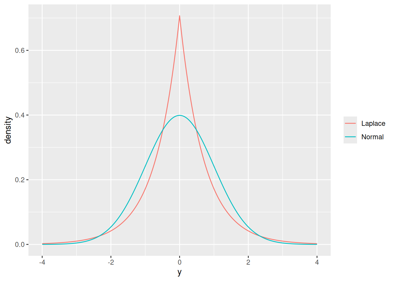
Remark. The normal density has the squared distance $(y - \mu)^2$ in its exponent. The Laplace density has the absolute distance $\mathopen{}\left|y - \mu\right|\mathclose{}$ instead. Both densities are symmetric about $\mu$, but the Laplace density has a sharp peak at $\mu$ and decays more slowly in the tails.

Example 14 (Laplace density values)

Example 14 (Laplace density values) Let $Y \sim {\operatorname{Laplace}\mathopen{}\left(3, 2\right)\mathclose{}}$, so $\mu= 3$ and $b = 2$ (Definition 7). At the location, $\mathopen{}\left|y - \mu\right|\mathclose{} = 0$, so the density is $\frac{1}{2b}$. At a point $y = 5$, the distance is

\[ \begin{aligned} \mathopen{}\left|5 - 3\right|\mathclose{} &= 2 \\ &= b, \end{aligned} \]

so the density is $\frac{1}{2b}\text{e}^{-1}$. Here are both values:

b <- 2
c(
  at_mu = 1 / (2 * b),
  at_mu_plus_2 = exp(-1) / (2 * b)
) |>
  round(3)
#>        at_mu at_mu_plus_2 
#>        0.250        0.092

The density at $\mu+ b$ is the density at $\mu$ times $\text{e}^{-1}$, and the same holds at $\mu- b$, because the density depends only on the distance from $\mu$.

Theorem 12 (Mean and variance of the Laplace distribution)

Theorem 12 (Mean and variance of the Laplace distribution) If $Y \sim {\operatorname{Laplace}\mathopen{}\left(\mu, b\right)\mathclose{}}$ (Definition 7), then

\[{\mathbb{E}\mathopen{}\left[Y\right]\mathclose{}} = \mu\quad \text{and} \quad {\operatorname{Var}\mathopen{}\left(Y\right)\mathclose{}} = 2b^2. \tag{7}\]

Proof

Proof. Write $U = Y - \mu$. By Equation 6, $U$ has density $\frac{1}{2b}\text{e}^{-\mathopen{}\left|u\right|\mathclose{}/b}$, which is symmetric about $0$.

For the mean, the integrand $u \cdot \frac{1}{2b}\text{e}^{-\mathopen{}\left|u\right|\mathclose{}/b}$ is an odd function, so its integral over $\mathbb{R}$ is $0$. Therefore ${\mathbb{E}\mathopen{}\left[U\right]\mathclose{}} = 0$, and

\[ \begin{aligned} {\mathbb{E}\mathopen{}\left[Y\right]\mathclose{}} &= \mu+ {\mathbb{E}\mathopen{}\left[U\right]\mathclose{}} \\ &= \mu. \end{aligned} \]

For the variance,

\[ \begin{aligned} {\operatorname{Var}\mathopen{}\left(Y\right)\mathclose{}} &= {\operatorname{Var}\mathopen{}\left(U\right)\mathclose{}} \\ &= {\mathbb{E}\mathopen{}\left[U^2\right]\mathclose{}} \end{aligned} \]

because ${\mathbb{E}\mathopen{}\left[U\right]\mathclose{}} = 0$. The integrand $u^2 \cdot \frac{1}{2b}\text{e}^{-\mathopen{}\left|u\right|\mathclose{}/b}$ is even, so

\[ \begin{aligned} {\mathbb{E}\mathopen{}\left[U^2\right]\mathclose{}} &= 2 \int_0^\infty u^2 \frac{1}{2b} \text{e}^{-u/b} \, du && \text{(even integrand)} \\ &= \frac{1}{b} \int_0^\infty u^2 \text{e}^{-u/b} \, du && \text{(multiplying the constants)} \\ &= \frac{1}{b} \mathopen{}\left(2b \int_0^\infty u \text{e}^{-u/b} \, du\right)\mathclose{} && \text{(integration by parts; the boundary terms are $0$)} \\ &= \frac{1}{b} \mathopen{}\left(2b \cdot b^2\right)\mathclose{} && \text{(integration by parts again; the boundary terms are $0$)} \\ &= 2b^2. && \text{(multiplying the constants)} \end{aligned} \]

Example 15 (Laplace and normal tails with the same mean and variance)

Example 15 (Laplace and normal tails with the same mean and variance) A Laplace variable $Y \sim {\operatorname{Laplace}\mathopen{}\left(0, b\right)\mathclose{}}$ has variance $2b^2$ (Theorem 12). Choosing $b = 1/\sqrt{2}$ gives variance $1$, the same mean and variance as a standard normal. Figure 3 compares the two densities. The Laplace density is higher at the center and in the far tails, and lower in between.

Show code

b <- 1 / sqrt(2)
grid <- seq(-4, 4, length.out = 801)
dlaplace <- function(y, mu = 0, b = 1) exp(-abs(y - mu) / b) / (2 * b)
densities <- tibble::tibble(
  y = rep(grid, times = 2),
  distribution = rep(c("Laplace", "Normal"), each = length(grid)),
  density = c(dlaplace(grid, b = b), dnorm(grid))
)
ggplot2::ggplot(densities) +
  ggplot2::aes(x = y, y = density, colour = distribution) +
  ggplot2::geom_line() +
  ggplot2::labs(colour = NULL)

Two symmetric curves over y from minus 4 to 4. The standard normal is a smooth bell. The Laplace curve with the same variance peaks higher at 0 with a sharp point, falls below the normal curve at moderate distances, and stays above it in the far tails. — Figure 3: Laplace and standard normal densities with the same mean (0) and variance (1)

The probability of landing more than $3$ standard deviations from the mean shows the difference in the tails. For the Laplace distribution, $\mathbb{P}(\mathopen{}\left|Y\right|\mathclose{} > t) = \text{e}^{-t/b}$, because each tail has probability $\frac{1}{2}\text{e}^{-t/b}$ by integrating Equation 6.

t <- 3
c(
  Laplace = exp(-t / b),
  Normal = 2 * pnorm(-t)
)
#>     Laplace      Normal 
#> 0.014369596 0.002699796

The Laplace distribution puts about 5.3 times as much probability beyond $3$ standard deviations as the normal distribution does.

6 The gamma distribution

Definition 8 (Gamma function)

Definition 8 (Gamma function) The gamma function $\Gamma$ is defined for each $s > 0$ by:

\[\Gamma(s) \stackrel{\text{def}}{=}\int_0^\infty u^{s - 1} \text{e}^{-u} \, du\]

Definition 9 (Gamma distribution)

Definition 9 (Gamma distribution) A non-negative random variable $T$ has the gamma distribution with shape $\alpha> 0$ and rate ${\lambda}> 0$, written $T \sim {\operatorname{Gam}\mathopen{}\left(\alpha, {\lambda}\right)\mathclose{}}$, if $T$ is continuous with density:

\[ f(t) \stackrel{\text{def}}{=}\begin{cases} \frac{{\lambda}^{\alpha}}{\Gamma(\alpha)} \, t^{\alpha- 1} \text{e}^{-{\lambda}t}, & t > 0 \\ 0, & t \le 0 \end{cases} \]

where $\Gamma$ is the gamma function.

Example 16 (Gamma density with shape 2)

Example 16 (Gamma density with shape 2) If $T \sim {\operatorname{Gam}\mathopen{}\left(2, {\lambda}\right)\mathclose{}}$, then $\Gamma(2) = 1$, so the density is:

\[ f(t) = {\lambda}^2 \, t \, \text{e}^{-{\lambda}t}, \quad t > 0 \]

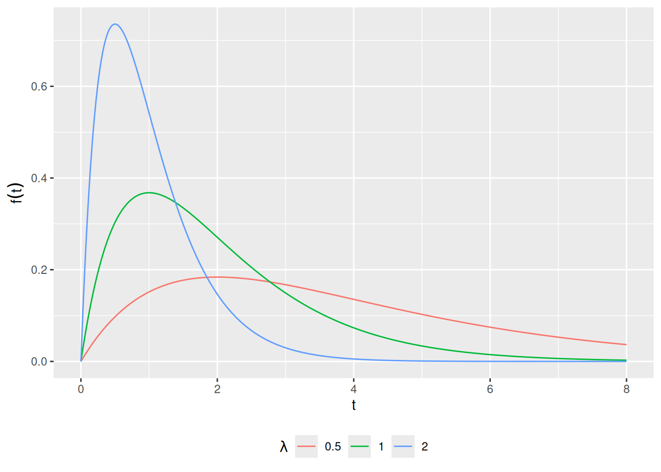
The density is $0$ at $t = 0$, rises to a peak at $t = 1/{\lambda}$, and then decays (Figure 4).

Show code

rates <- c(0.5, 1, 2)
t_grid <- seq(0, 8, length.out = 400)
rate_label <- latex2exp::TeX("$\\lambda$")
density_label <- latex2exp::TeX("$f(t)$")

gamma_densities <-
  dplyr::tibble(rate = rates) |>
  dplyr::reframe(.by = rate, t = t_grid) |>
  dplyr::mutate(
    density = dgamma(t, shape = 2, rate = rate),
    rate = factor(rate)
  )

gamma_plot <-
  gamma_densities |>
  ggplot2::ggplot() +
  ggplot2::aes(x = t, y = density, col = rate) +
  ggplot2::geom_line() +
  ggplot2::labs(col = rate_label, y = density_label) +
  ggplot2::theme(legend.position = "bottom")

print(gamma_plot)

Gamma densities with shape 2 rise from zero, peak, then decay. — Figure 4: Gamma densities with shape 2, by rate ${\lambda}$

Theorem 13 (Moments of the gamma distribution)

Theorem 13 (Moments of the gamma distribution) If $T \sim {\operatorname{Gam}\mathopen{}\left(\alpha, {\lambda}\right)\mathclose{}}$, then for every integer $k \ge 0$:

\[{\mathbb{E}\mathopen{}\left[T^k\right]\mathclose{}} = \frac{\Gamma(\alpha+ k)}{\Gamma(\alpha) \, {\lambda}^k}\]

Proof

Proof. The substitution below reduces the expectation to the gamma function:

\[ \begin{aligned} {\mathbb{E}\mathopen{}\left[T^k\right]\mathclose{}} &= \int_0^\infty t^k \, \frac{{\lambda}^{\alpha}}{\Gamma(\alpha)} \, t^{\alpha- 1} \text{e}^{-{\lambda}t} \, dt && (\text{definition of expectation, with the gamma density}) \\ &= \frac{{\lambda}^{\alpha}}{\Gamma(\alpha)} \int_0^\infty t^{\alpha+ k - 1} \text{e}^{-{\lambda}t} \, dt && (t^k \cdot t^{\alpha- 1} = t^{\alpha+ k - 1}) \\ &= \frac{{\lambda}^{\alpha}}{\Gamma(\alpha)} \cdot \frac{1}{{\lambda}^{\alpha+ k}} \int_0^\infty u^{\alpha+ k - 1} \text{e}^{-u} \, du && (\text{substitute } u = {\lambda}t) \\ &= \frac{{\lambda}^{\alpha}}{\Gamma(\alpha)} \cdot \frac{\Gamma(\alpha+ k)}{{\lambda}^{\alpha+ k}} && (\text{definition of } \Gamma) \\ &= \frac{\Gamma(\alpha+ k)}{\Gamma(\alpha) \, {\lambda}^k} && ({\lambda}^{\alpha} / {\lambda}^{\alpha+ k} = {\lambda}^{-k}) \end{aligned} \]

Corollary 1 (Mean of the gamma distribution)

Corollary 1 (Mean of the gamma distribution) If $T \sim {\operatorname{Gam}\mathopen{}\left(\alpha, {\lambda}\right)\mathclose{}}$, then ${\mathbb{E}\mathopen{}\left[T\right]\mathclose{}} = \alpha/ {\lambda}$.

Proof

Proof. By Theorem 13 with $k = 1$:

\[ \begin{aligned} {\mathbb{E}\mathopen{}\left[T\right]\mathclose{}} &= \frac{\Gamma(\alpha+ 1)}{\Gamma(\alpha) \, {\lambda}} && (\text{moment formula with } k = 1) \\ &= \frac{\alpha\, \Gamma(\alpha)}{\Gamma(\alpha) \, {\lambda}} && (\Gamma(\alpha+ 1) = \alpha\, \Gamma(\alpha)) \\ &= \frac{\alpha}{{\lambda}} && (\text{cancel } \Gamma(\alpha)) \end{aligned} \]

Corollary 2 (Variance of the gamma distribution)

Corollary 2 (Variance of the gamma distribution) If $T \sim {\operatorname{Gam}\mathopen{}\left(\alpha, {\lambda}\right)\mathclose{}}$, then ${\operatorname{Var}\mathopen{}\left(T\right)\mathclose{}} = \alpha/ {\lambda}^2$.

Proof

Proof. First, the second moment, by Theorem 13 with $k = 2$:

\[ \begin{aligned} {\mathbb{E}\mathopen{}\left[T^2\right]\mathclose{}} &= \frac{\Gamma(\alpha+ 2)}{\Gamma(\alpha) \, {\lambda}^2} && (\text{moment formula with } k = 2) \\ &= \frac{(\alpha+ 1) \, \Gamma(\alpha+ 1)}{\Gamma(\alpha) \, {\lambda}^2} && (\Gamma(\alpha+ 2) = (\alpha+ 1) \, \Gamma(\alpha+ 1)) \\ &= \frac{(\alpha+ 1) \, \alpha\, \Gamma(\alpha)}{\Gamma(\alpha) \, {\lambda}^2} && (\Gamma(\alpha+ 1) = \alpha\, \Gamma(\alpha)) \\ &= \frac{\alpha(\alpha+ 1)}{{\lambda}^2} && (\text{cancel } \Gamma(\alpha)) \end{aligned} \]

Then, by the simplified expression for variance and Corollary 1:

\[ \begin{aligned} {\operatorname{Var}\mathopen{}\left(T\right)\mathclose{}} &= {\mathbb{E}\mathopen{}\left[T^2\right]\mathclose{}} - {\mathopen{}\left({\mathbb{E}\mathopen{}\left[T\right]\mathclose{}}\right)\mathclose{}}^{2} && (\text{simplified expression for variance}) \\ &= \frac{\alpha(\alpha+ 1)}{{\lambda}^2} - \frac{\alpha^2}{{\lambda}^2} && (\text{mean of the gamma distribution}) \\ &= \frac{\alpha^2 + \alpha- \alpha^2}{{\lambda}^2} && (\text{expand } \alpha(\alpha+ 1) \text{ and combine fractions}) \\ &= \frac{\alpha}{{\lambda}^2} && (\alpha^2 - \alpha^2 = 0) \end{aligned} \]

Corollary 3 (The gamma distribution with shape 1 is the exponential)

Corollary 3 (The gamma distribution with shape 1 is the exponential) If $T \sim {\operatorname{Gam}\mathopen{}\left(1, {\lambda}\right)\mathclose{}}$, then $T$ has the exponential distribution with rate ${\lambda}$.

Proof

Proof. For $t > 0$:

\[ \begin{aligned} f(t) &= \frac{{\lambda}^{1}}{\Gamma(1)} \, t^{1 - 1} \text{e}^{-{\lambda}t} && (\text{gamma density with } \alpha= 1) \\ &= {\lambda}\, t^{0} \text{e}^{-{\lambda}t} && (\Gamma(1) = 1 \text{ and } 1 - 1 = 0) \\ &= {\lambda}\text{e}^{-{\lambda}t} && (t^0 = 1) \end{aligned} \]

and $f(t) = 0$ for $t \le 0$. This density is the exponential density with rate ${\lambda}$.

7 Weibull distribution

Definition 10 (Weibull distribution)

Definition 10 (Weibull distribution) A non-negative random variable $T$ has the Weibull distribution with shape $\alpha> 0$ and rate ${\lambda}> 0$ [6] if its survival function is:

\[\mathbb{S}(t) \stackrel{\text{def}}{=}\text{e}^{-{\lambda}t^\alpha}, \quad t \ge 0\]

Theorem 14 (Weibull density and hazard)

Theorem 14 (Weibull density and hazard) If $T$ has the Weibull distribution with shape $\alpha$ and rate ${\lambda}$, then for $t > 0$:

\[ \begin{aligned} f(t) &= \alpha{\lambda}t^{\alpha-1}\text{e}^{-{\lambda}t^\alpha}\\ \mathbb{h}(t) &= \alpha{\lambda}t^{\alpha-1} \end{aligned} \]

Proof

Proof. The CDF of $T$ is $F(t) = 1 - \mathbb{S}(t)$ (survival function and CDF), which is $0$ for $t < 0$ and $1 - \text{e}^{-{\lambda}t^\alpha}$ for $t \ge 0$. This $F$ is continuous everywhere, with a continuous derivative everywhere except possibly $t = 0$, so

\[ \begin{aligned} f &= F' \\ &= -\mathbb{S}' \end{aligned} \]

is a density of $T$ (a piecewise-smooth CDF has its derivative as a density). This density is continuous at every $t > 0$, so there the hazard is $f(t)/\mathbb{S}(t)$ (hazard equals density over survival):

\[ \begin{aligned} f(t) &= -\frac{d}{dt}\text{e}^{-{\lambda}t^\alpha} && (f = -\mathbb{S}') \\ &= \alpha{\lambda}t^{\alpha-1}\text{e}^{-{\lambda}t^\alpha} && (\text{chain rule}) \\ \mathbb{h}(t) &= \frac{\alpha{\lambda}t^{\alpha-1}\text{e}^{-{\lambda}t^\alpha}}{\text{e}^{-{\lambda}t^\alpha}} && (\text{hazard is density over survival}) \\ &= \alpha{\lambda}t^{\alpha-1} && (\text{cancel}) \end{aligned} \]

Remark

Remark. The hazard is written $\mathbb{h}(t)$ here, rather than ${\lambda}(t)$, because the Weibull rate parameter is also called ${\lambda}$.

Theorem 15 (Weibull mean)

Theorem 15 (Weibull mean) If $T$ has the Weibull distribution with shape $\alpha$ and rate ${\lambda}$, then:

\[{\mathbb{E}\mathopen{}\left[T\right]\mathclose{}} = \Gamma(1+1/\alpha)\cdot {\lambda}^{-1/\alpha}\]

Proof

Proof. For the mean, use the survival-function formula for the mean and substitute $u = {\lambda}t^\alpha$, so that $t = (u/{\lambda})^{1/\alpha}$ and $dt = \frac{1}{\alpha}{\lambda}^{-1/\alpha} u^{1/\alpha- 1}\,du$:

\[ \begin{aligned} {\mathbb{E}\mathopen{}\left[T\right]\mathclose{}} &= \int_0^\infty \text{e}^{-{\lambda}t^\alpha}\,dt && (\text{expectation via the survival function}) \\ &= \frac{1}{\alpha}{\lambda}^{-1/\alpha} \int_0^\infty u^{1/\alpha- 1} \text{e}^{-u}\,du && (\text{substitute } u = {\lambda}t^\alpha) \\ &= \frac{1}{\alpha}{\lambda}^{-1/\alpha}\,\Gamma(1/\alpha) && (\text{definition of the gamma function}) \\ &= \Gamma(1 + 1/\alpha)\,{\lambda}^{-1/\alpha} && (\Gamma(1 + a) = a\,\Gamma(a)) \end{aligned} \]

Corollary 4 (The Weibull with shape 1 is the exponential)

Corollary 4 (The Weibull with shape 1 is the exponential) If $T$ has the Weibull distribution with shape $\alpha= 1$ and rate ${\lambda}$, then $T$ has the exponential distribution with rate ${\lambda}$.

Proof

Proof. By Theorem 14 with $\alpha= 1$, for $t > 0$:

\[ \begin{aligned} f(t) &= \alpha{\lambda}t^{\alpha-1}\text{e}^{-{\lambda}t^\alpha} && (\text{Weibull density}) \\ &= 1 \cdot {\lambda}t^{0}\text{e}^{-{\lambda}t^1} && (\text{substitute } \alpha= 1) \\ &= {\lambda}\text{e}^{-{\lambda}t} && (t^0 = 1 \text{ and } t^1 = t) \end{aligned} \]

and $f(t) = 0$ for $t < 0$, since $T$ is non-negative. This density matches the exponential density at every $t \ne 0$. Changing a density at the single point $t = 0$ does not change its integral over any set, so $T$ has the exponential distribution with rate ${\lambda}$.

Corollary 5 (The Weibull shape sets the direction of the hazard)

Corollary 5 (The Weibull shape sets the direction of the hazard) If $T$ has the Weibull distribution with shape $\alpha$ and rate ${\lambda}$, then on $t > 0$ its hazard $\mathbb{h}(t)$ is:

strictly increasing if $\alpha> 1$
constant if $\alpha= 1$
strictly decreasing if $\alpha< 1$

Proof

Proof. By Theorem 14, $\mathbb{h}(t) = \alpha{\lambda}t^{\alpha-1}$ for $t > 0$, so:

\[ \begin{aligned} \frac{d}{dt}\mathbb{h}(t) &= \frac{d}{dt} \alpha{\lambda}t^{\alpha-1} && (\text{Weibull hazard}) \\ &= \alpha(\alpha- 1){\lambda}t^{\alpha-2} && (\text{power rule}) \end{aligned} \]

For $t > 0$, the factors $\alpha$, ${\lambda}$, and $t^{\alpha-2}$ are all positive, so $\frac{d}{dt}\mathbb{h}(t)$ has the sign of $\alpha- 1$: positive for $\alpha> 1$, zero for $\alpha= 1$, and negative for $\alpha< 1$. A function with a positive (negative) derivative on an interval is strictly increasing (decreasing) there, and one with a zero derivative is constant.

Remark

Remark. The exponential distribution’s hazard is constant, so the Weibull’s choice of an increasing, constant, or decreasing hazard (Corollary 5) provides more flexibility than the exponential.

Example 17 (Exponential as a special case)

Example 17 (Exponential as a special case) With $\alpha= 1$, Theorem 14 gives $\mathbb{h}(t) = {\lambda}$ and

\[ \begin{aligned} {\mathbb{E}\mathopen{}\left[T\right]\mathclose{}} &= \Gamma(2){\lambda}^{-1} \\ &= 1/{\lambda}, \end{aligned} \]

matching the exponential distribution’s constant hazard and mean. With $\alpha= 2$ and ${\lambda}= 1$, $\mathbb{h}(t) = 2t$ increases with $t$, and

\[ \begin{aligned} {\mathbb{E}\mathopen{}\left[T\right]\mathclose{}} &= \Gamma(3/2) \\ &= \sqrt{\pi}/2 \\ &\approx 0.886. \end{aligned} \]

8 The multivariate normal distribution

Definition 11 (Multivariate normal distribution (multivariate Gaussian distribution))

Definition 11 (Multivariate normal distribution (multivariate Gaussian distribution)) A $p \times 1$ random vector $\mathord{\smash[b]{\underset{\raise.3ex\hbox{$\scriptstyle\sim$}}{X}}\vphantom{X}}= {(X_1, \ldots, X_p)}^{\top}$ has the multivariate normal distribution (or multivariate Gaussian distribution) with mean parameter $\mathord{\smash[b]{\underset{\raise.3ex\hbox{$\scriptstyle\sim$}}{\mu}}\vphantom{\mu}} \in \mathbb{R}^p$ and variance parameter $\mathbf{\Sigma}$, a $p \times p$ positive definite matrix, written $\mathord{\smash[b]{\underset{\raise.3ex\hbox{$\scriptstyle\sim$}}{X}}\vphantom{X}}\sim \operatorname{N}_p\mathopen{}\left(\mathord{\smash[b]{\underset{\raise.3ex\hbox{$\scriptstyle\sim$}}{\mu}}\vphantom{\mu}}, \mathbf{\Sigma}\right)\mathclose{}$, if $\mathord{\smash[b]{\underset{\raise.3ex\hbox{$\scriptstyle\sim$}}{X}}\vphantom{X}}$ has joint density:

\[ \mathbb{p}(\mathord{\smash[b]{\underset{\raise.3ex\hbox{$\scriptstyle\sim$}}{X}}\vphantom{X}}= \mathord{\smash[b]{\underset{\raise.3ex\hbox{$\scriptstyle\sim$}}{x}}\vphantom{x}}) \stackrel{\text{def}}{=} \frac{1}{(2\pi)^{p/2} \det(\mathbf{\Sigma})^{1/2}} \text{e}^{-\frac{1}{2} {(\mathord{\smash[b]{\underset{\raise.3ex\hbox{$\scriptstyle\sim$}}{x}}\vphantom{x}}- \mathord{\smash[b]{\underset{\raise.3ex\hbox{$\scriptstyle\sim$}}{\mu}}\vphantom{\mu}})}^{\top} \mathbf{\Sigma}^{-1} (\mathord{\smash[b]{\underset{\raise.3ex\hbox{$\scriptstyle\sim$}}{x}}\vphantom{x}}- \mathord{\smash[b]{\underset{\raise.3ex\hbox{$\scriptstyle\sim$}}{\mu}}\vphantom{\mu}})}, \quad \mathord{\smash[b]{\underset{\raise.3ex\hbox{$\scriptstyle\sim$}}{x}}\vphantom{x}}\in \mathbb{R}^p \]

where $\det(\mathbf{\Sigma})$ is the determinant of $\mathbf{\Sigma}$ and $\mathbf{\Sigma}^{-1}$ is its inverse.

Example 18 (A bivariate Gaussian density)

Example 18 (A bivariate Gaussian density) Let $p = 2$, $\mathord{\smash[b]{\underset{\raise.3ex\hbox{$\scriptstyle\sim$}}{\mu}}\vphantom{\mu}} = \mathord{\smash[b]{\underset{\raise.3ex\hbox{$\scriptstyle\sim$}}{0}}\vphantom{0}}$, and $\mathbf{\Sigma} = \begin{pmatrix}1 & 0.8 \\ 0.8 & 1\end{pmatrix}$. Then $\det(\mathbf{\Sigma}) = 1 - 0.8^2 = 0.36$, so the density of $\mathord{\smash[b]{\underset{\raise.3ex\hbox{$\scriptstyle\sim$}}{X}}\vphantom{X}}\sim \operatorname{N}_2\mathopen{}\left(\mathord{\smash[b]{\underset{\raise.3ex\hbox{$\scriptstyle\sim$}}{0}}\vphantom{0}}, \mathbf{\Sigma}\right)\mathclose{}$ (multivariate Gaussian) at the mean, which is also its peak, is:

\[ \begin{aligned} {\mathbb{p}\mathopen{}\left(\mathord{\smash[b]{\underset{\raise.3ex\hbox{$\scriptstyle\sim$}}{0}}\vphantom{0}}\right)\mathclose{}} &= \frac{1}{2\pi \cdot 0.36^{1/2}} \text{e}^{0} && \text{(substitute into the multivariate normal density)} \\ &= \frac{1}{0.6 \cdot 2\pi} && \text{(simplify)} \end{aligned} \]

which is about 0.265. The density is a bell-shaped surface over the $(x_1, x_2)$ plane (Figure 5). Because $\mathbf{\Sigma}_{12} = 0.8 > 0$, the surface is stretched along the line $x_2 = x_1$.

Show code

viewof mbMean1 = Inputs.range([-2, 2], {value: 0, step: 0.1, label: "mean of X1"})
viewof mbMean2 = Inputs.range([-2, 2], {value: 0, step: 0.1, label: "mean of X2"})
viewof mbVar1 = Inputs.range([0.2, 3], {value: 1, step: 0.05, label: "variance of X1"})
viewof mbVar2 = Inputs.range([0.2, 3], {value: 1, step: 0.05, label: "variance of X2"})
viewof mbCor = Inputs.range([-0.95, 0.95], {value: 0.8, step: 0.05, label: "correlation"})

Show code

mbCov = mbCor * Math.sqrt(mbVar1 * mbVar2)
mbPeak = 1 / (2 * Math.PI * Math.sqrt(mbVar1 * mbVar2 - mbCov * mbCov))
md`Covariance: ${mbCov.toFixed(3)}. Density at the mean: ${mbPeak.toFixed(3)}.`

Show code

// One div that every redraw reuses, so a rotated view stays rotated.
mbDiv = html`<div role="img" aria-label="Surface plot of a bivariate Gaussian density over x1 and x2, redrawn for the means, variances and correlation chosen with the sliders. At the starting values it is a single bell-shaped peak of height about 0.265 at the origin, stretched along the line x2 = x1." style="width:100%;height:450px"></div>`

Show code

{
  // The density over the grid; row j holds x2 = mbGrid[j], as plotly expects.
  const det = mbVar1 * mbVar2 - mbCov * mbCov;
  const z = mbGrid.map((x2) => mbGrid.map((x1) => {
    const d1 = x1 - mbMean1;
    const d2 = x2 - mbMean2;
    const quad = (mbVar2 * d1 * d1 - 2 * mbCov * d1 * d2 + mbVar1 * d2 * d2) / det;
    return mbPeak * Math.exp(-quad / 2);
  }));
  const surface = {
    type: "surface", x: mbGrid, y: mbGrid, z: z,
    colorscale: [[0, "#CCE0F0"], [1, "#0072B2"]],
    showscale: false, opacity: 0.9
  };
  const layout = {
    // A constant uirevision keeps the reader's camera angle across redraws.
    uirevision: "keep",
    margin: {l: 0, r: 0, t: 0, b: 0},
    scene: {
      aspectmode: "cube",
      xaxis: {title: {text: "x1"}},
      yaxis: {title: {text: "x2"}},
      zaxis: {title: {text: "density"}},
      camera: {eye: {x: 1.6, y: -1.6, z: 0.9}}
    }
  };
  mbPlotly.react(mbDiv, [surface], layout);
}

Figure 5: The density of $\operatorname{N}_2\mathopen{}\left(\mathord{\smash[b]{\underset{\raise.3ex\hbox{$\scriptstyle\sim$}}{0}}\vphantom{0}}, \mathbf{\Sigma}\right)\mathclose{}$ in the example, with variances $1$ and covariance $0.8$. Its horizontal slices are ellipses stretched along $x_2 = x_1$.

Remark

Remark. A joint density of $p$ random variables is the $p$-variable analogue of a joint density of two: a non-negative function on $\mathbb{R}^p$ whose integral over any region $A \subseteq \mathbb{R}^p$ is $\Pr(\mathord{\smash[b]{\underset{\raise.3ex\hbox{$\scriptstyle\sim$}}{X}}\vphantom{X}}\in A)$.

The density is well defined because $\mathbf{\Sigma}$ is positive definite:

$\mathbf{\Sigma}^{-1}$ exists (positive definite matrices have positive definite inverses), and
$\det(\mathbf{\Sigma}) > 0$ (positive definite matrices have positive determinants), so its square root is a positive number.

Theorem 16 (The multivariate normal density integrates to 1)

Theorem 16 (The multivariate normal density integrates to 1) If $\mathord{\smash[b]{\underset{\raise.3ex\hbox{$\scriptstyle\sim$}}{X}}\vphantom{X}}\sim \operatorname{N}_p\mathopen{}\left(\mathord{\smash[b]{\underset{\raise.3ex\hbox{$\scriptstyle\sim$}}{\mu}}\vphantom{\mu}}, \mathbf{\Sigma}\right)\mathclose{}$ (Definition 11), then the density in Definition 11 integrates to 1 over $\mathbb{R}^p$.

Theorem 17 (The mean and variance of the multivariate normal distribution)

Theorem 17 (The mean and variance of the multivariate normal distribution) If $\mathord{\smash[b]{\underset{\raise.3ex\hbox{$\scriptstyle\sim$}}{X}}\vphantom{X}}\sim \operatorname{N}_p\mathopen{}\left(\mathord{\smash[b]{\underset{\raise.3ex\hbox{$\scriptstyle\sim$}}{\mu}}\vphantom{\mu}}, \mathbf{\Sigma}\right)\mathclose{}$ (Definition 11), then $\mathbb{E}\mathord{\smash[b]{\underset{\raise.3ex\hbox{$\scriptstyle\sim$}}{X}}\vphantom{X}}= \mathord{\smash[b]{\underset{\raise.3ex\hbox{$\scriptstyle\sim$}}{\mu}}\vphantom{\mu}}$ (the expectation of a random vector), and ${\operatorname{Var}\mathopen{}\left(\mathord{\smash[b]{\underset{\raise.3ex\hbox{$\scriptstyle\sim$}}{X}}\vphantom{X}}\right)\mathclose{}} = \mathbf{\Sigma}$ (the variance of a random vector).

Remark

Remark. The proof changes variables in a $p$-dimensional integral, which these notes do not develop; see [7]. As with the univariate normal distribution, these facts are where the parameters’ names come from. They also show why $\mathbf{\Sigma}$ must at least be positive semidefinite; requiring it to be positive definite rules out cases like a variance matrix that is not positive definite, which has no joint density.

Example 19 (The univariate normal is the case $p = 1$)

Example 19 (The univariate normal is the case $p = 1$) With $p = 1$, $\mathord{\smash[b]{\underset{\raise.3ex\hbox{$\scriptstyle\sim$}}{\mu}}\vphantom{\mu}} = (\mu)$, and $\mathbf{\Sigma} = (\sigma^2)$ for $\sigma^2> 0$, $\det(\mathbf{\Sigma}) = \sigma^2$ (determinant, $p = 1$) and $\mathbf{\Sigma}^{-1} = (1/\sigma^2)$, so:

\[ \begin{aligned} \mathbb{p}(\mathord{\smash[b]{\underset{\raise.3ex\hbox{$\scriptstyle\sim$}}{X}}\vphantom{X}}= \mathord{\smash[b]{\underset{\raise.3ex\hbox{$\scriptstyle\sim$}}{x}}\vphantom{x}}) &= \frac{1}{(2\pi)^{1/2} (\sigma^2)^{1/2}} \text{e}^{-\frac{1}{2} (x - \mu) \frac{1}{\sigma^2} (x - \mu)} && \text{(substitute into the multivariate normal density)} \\ &= \frac{1}{\sigma\sqrt{2\pi}} \text{e}^{-\frac{(x - \mu)^2}{2\sigma^2}} && \text{(simplify)} \end{aligned} \]

which is the normal density ${\operatorname{N}\mathopen{}\left(\mu, \sigma^2\right)\mathclose{}}$.

Lemma 1 (The quadratic form in the multivariate normal density is non-negative)

Lemma 1 (The quadratic form in the multivariate normal density is non-negative) If $\mathbf{\Sigma}$ is a $p \times p$ positive definite matrix and $\mathord{\smash[b]{\underset{\raise.3ex\hbox{$\scriptstyle\sim$}}{x}}\vphantom{x}}, \mathord{\smash[b]{\underset{\raise.3ex\hbox{$\scriptstyle\sim$}}{\mu}}\vphantom{\mu}} \in \mathbb{R}^p$, then

\[{(\mathord{\smash[b]{\underset{\raise.3ex\hbox{$\scriptstyle\sim$}}{x}}\vphantom{x}}- \mathord{\smash[b]{\underset{\raise.3ex\hbox{$\scriptstyle\sim$}}{\mu}}\vphantom{\mu}})}^{\top} \mathbf{\Sigma}^{-1} (\mathord{\smash[b]{\underset{\raise.3ex\hbox{$\scriptstyle\sim$}}{x}}\vphantom{x}}- \mathord{\smash[b]{\underset{\raise.3ex\hbox{$\scriptstyle\sim$}}{\mu}}\vphantom{\mu}}) \ge 0,\]

with equality if and only if $\mathord{\smash[b]{\underset{\raise.3ex\hbox{$\scriptstyle\sim$}}{x}}\vphantom{x}}= \mathord{\smash[b]{\underset{\raise.3ex\hbox{$\scriptstyle\sim$}}{\mu}}\vphantom{\mu}}$.

Proof

Proof. $\mathbf{\Sigma}^{-1}$ is positive definite (positive definite inverse). If $\mathord{\smash[b]{\underset{\raise.3ex\hbox{$\scriptstyle\sim$}}{x}}\vphantom{x}}\neq \mathord{\smash[b]{\underset{\raise.3ex\hbox{$\scriptstyle\sim$}}{\mu}}\vphantom{\mu}}$, then $\mathord{\smash[b]{\underset{\raise.3ex\hbox{$\scriptstyle\sim$}}{x}}\vphantom{x}}- \mathord{\smash[b]{\underset{\raise.3ex\hbox{$\scriptstyle\sim$}}{\mu}}\vphantom{\mu}} \neq \mathord{\smash[b]{\underset{\raise.3ex\hbox{$\scriptstyle\sim$}}{0}}\vphantom{0}}$, so the quadratic form is positive by the definition of positive definite. If $\mathord{\smash[b]{\underset{\raise.3ex\hbox{$\scriptstyle\sim$}}{x}}\vphantom{x}}= \mathord{\smash[b]{\underset{\raise.3ex\hbox{$\scriptstyle\sim$}}{\mu}}\vphantom{\mu}}$, then $\mathord{\smash[b]{\underset{\raise.3ex\hbox{$\scriptstyle\sim$}}{x}}\vphantom{x}}- \mathord{\smash[b]{\underset{\raise.3ex\hbox{$\scriptstyle\sim$}}{\mu}}\vphantom{\mu}} = \mathord{\smash[b]{\underset{\raise.3ex\hbox{$\scriptstyle\sim$}}{0}}\vphantom{0}}$, and the quadratic form is $0$.

Definition 12 (Mahalanobis distance)

Definition 12 (Mahalanobis distance) For a $p \times p$ positive definite matrix $\mathbf{\Sigma}$ and $\mathord{\smash[b]{\underset{\raise.3ex\hbox{$\scriptstyle\sim$}}{x}}\vphantom{x}}, \mathord{\smash[b]{\underset{\raise.3ex\hbox{$\scriptstyle\sim$}}{\mu}}\vphantom{\mu}} \in \mathbb{R}^p$, the Mahalanobis distance from $\mathord{\smash[b]{\underset{\raise.3ex\hbox{$\scriptstyle\sim$}}{x}}\vphantom{x}}$ to $\mathord{\smash[b]{\underset{\raise.3ex\hbox{$\scriptstyle\sim$}}{\mu}}\vphantom{\mu}}$ with respect to $\mathbf{\Sigma}$ is:

\[ \Delta(\mathord{\smash[b]{\underset{\raise.3ex\hbox{$\scriptstyle\sim$}}{x}}\vphantom{x}}) \stackrel{\text{def}}{=}\sqrt{{(\mathord{\smash[b]{\underset{\raise.3ex\hbox{$\scriptstyle\sim$}}{x}}\vphantom{x}}- \mathord{\smash[b]{\underset{\raise.3ex\hbox{$\scriptstyle\sim$}}{\mu}}\vphantom{\mu}})}^{\top} \mathbf{\Sigma}^{-1} (\mathord{\smash[b]{\underset{\raise.3ex\hbox{$\scriptstyle\sim$}}{x}}\vphantom{x}}- \mathord{\smash[b]{\underset{\raise.3ex\hbox{$\scriptstyle\sim$}}{\mu}}\vphantom{\mu}})} \]

Remark

Remark. The square root is defined by Lemma 1. See also [8].

Corollary 6 (The multivariate normal density decreases with Mahalanobis distance)

Corollary 6 (The multivariate normal density decreases with Mahalanobis distance) If $\mathord{\smash[b]{\underset{\raise.3ex\hbox{$\scriptstyle\sim$}}{X}}\vphantom{X}}\sim \operatorname{N}_p\mathopen{}\left(\mathord{\smash[b]{\underset{\raise.3ex\hbox{$\scriptstyle\sim$}}{\mu}}\vphantom{\mu}}, \mathbf{\Sigma}\right)\mathclose{}$, then:

where $\Delta$ is the Mahalanobis distance to $\mathord{\smash[b]{\underset{\raise.3ex\hbox{$\scriptstyle\sim$}}{\mu}}\vphantom{\mu}}$ with respect to $\mathbf{\Sigma}$ (Definition 12). So the density is highest at $\mathord{\smash[b]{\underset{\raise.3ex\hbox{$\scriptstyle\sim$}}{x}}\vphantom{x}}= \mathord{\smash[b]{\underset{\raise.3ex\hbox{$\scriptstyle\sim$}}{\mu}}\vphantom{\mu}}$, decreases as $\Delta(\mathord{\smash[b]{\underset{\raise.3ex\hbox{$\scriptstyle\sim$}}{x}}\vphantom{x}})$ increases, and is the same at every $\mathord{\smash[b]{\underset{\raise.3ex\hbox{$\scriptstyle\sim$}}{x}}\vphantom{x}}$ with the same $\Delta(\mathord{\smash[b]{\underset{\raise.3ex\hbox{$\scriptstyle\sim$}}{x}}\vphantom{x}})$.

Proof

Proof. Substitute Definition 12 into Definition 11. The function $\delta\mapsto \text{e}^{-\delta^2/2}$ decreases on $\delta\ge 0$, and by Lemma 1, $\Delta(\mathord{\smash[b]{\underset{\raise.3ex\hbox{$\scriptstyle\sim$}}{x}}\vphantom{x}}) = 0$ only at $\mathord{\smash[b]{\underset{\raise.3ex\hbox{$\scriptstyle\sim$}}{x}}\vphantom{x}}= \mathord{\smash[b]{\underset{\raise.3ex\hbox{$\scriptstyle\sim$}}{\mu}}\vphantom{\mu}}$.

Example 20 (Mahalanobis distance for diagonal variance matrices)

Example 20 (Mahalanobis distance for diagonal variance matrices) If $\mathbf{\Sigma}$ is diagonal with diagonal elements $\sigma^2_1, \ldots, \sigma^2_p$, all positive, then $\mathbf{\Sigma}^{-1}$ is diagonal with diagonal elements $1/\sigma^2_1, \ldots, 1/\sigma^2_p$ (multiplying the two gives $\mathbf{I}_p$; matrix inverse), so:

\[ \Delta(\mathord{\smash[b]{\underset{\raise.3ex\hbox{$\scriptstyle\sim$}}{x}}\vphantom{x}})^2 = \sum_{i=1}^p\frac{(x_i - \mu_i)^2}{\sigma^2_i} \]

Two special cases:

If $\mathbf{\Sigma} = \mathbf{I}_p$, then $\Delta(\mathord{\smash[b]{\underset{\raise.3ex\hbox{$\scriptstyle\sim$}}{x}}\vphantom{x}})^2 = \sum_{i=1}^p(x_i - \mu_i)^2$, so the Mahalanobis distance is the ordinary (Euclidean) distance.
If $\mathbf{\Sigma} = \sigma^2\mathbf{I}_p$, then $\Delta(\mathord{\smash[b]{\underset{\raise.3ex\hbox{$\scriptstyle\sim$}}{x}}\vphantom{x}})$ is the Euclidean distance divided by $\sigma$.

In general, each coordinate’s difference is measured in units of that coordinate’s standard deviation.

Theorem 18 (A multivariate normal vector with diagonal variance has independent normal components)

Theorem 18 (A multivariate normal vector with diagonal variance has independent normal components) If $\mathord{\smash[b]{\underset{\raise.3ex\hbox{$\scriptstyle\sim$}}{X}}\vphantom{X}}\sim \operatorname{N}_p\mathopen{}\left(\mathord{\smash[b]{\underset{\raise.3ex\hbox{$\scriptstyle\sim$}}{\mu}}\vphantom{\mu}}, \mathbf{\Sigma}\right)\mathclose{}$ and $\mathbf{\Sigma}$ is diagonal with diagonal elements $\sigma^2_1, \ldots, \sigma^2_p$, then:

the joint density of $\mathord{\smash[b]{\underset{\raise.3ex\hbox{$\scriptstyle\sim$}}{X}}\vphantom{X}}$ is the product of the normal densities ${\operatorname{N}\mathopen{}\left(\mu_i, \sigma^2_i\right)\mathclose{}}$, $i = 1, \ldots, p$,
each $X_i \sim {\operatorname{N}\mathopen{}\left(\mu_i, \sigma^2_i\right)\mathclose{}}$, and
$X_1, \ldots, X_p$ are independent.

Proof

Proof. By the determinant of a diagonal matrix, $\det(\mathbf{\Sigma}) = \prod_{i=1}^p \sigma^2_i$, so $\det(\mathbf{\Sigma})^{1/2} = \prod_{i=1}^p \sigma_i$. Using Example 20 for the quadratic form:

\[ \begin{aligned} \mathbb{p}(\mathord{\smash[b]{\underset{\raise.3ex\hbox{$\scriptstyle\sim$}}{X}}\vphantom{X}}= \mathord{\smash[b]{\underset{\raise.3ex\hbox{$\scriptstyle\sim$}}{x}}\vphantom{x}}) &= \frac{1}{(2\pi)^{p/2} \prod_{i=1}^p \sigma_i} \text{e}^{-\frac{1}{2} \sum_{i=1}^p\frac{(x_i - \mu_i)^2}{\sigma^2_i}} && \text{(substitute)} \\ &= \prod_{i=1}^p \frac{1}{\sigma_i \sqrt{2\pi}} \text{e}^{-\frac{(x_i - \mu_i)^2}{2\sigma^2_i}} && \text{(} \text{e}^{a + b} = \text{e}^{a}\text{e}^{b} \text{)} \end{aligned} \]

which is the product of the ${\operatorname{N}\mathopen{}\left(\mu_i, \sigma^2_i\right)\mathclose{}}$ densities. Integrating out every coordinate except $x_i$, each other factor integrates to 1 (the normal density integrates to 1), leaving the ${\operatorname{N}\mathopen{}\left(\mu_i, \sigma^2_i\right)\mathclose{}}$ density as the density of $X_i$ (marginal density from a joint density, with $p$ variables). So the joint density is the product of the marginal densities, and the components are independent by the factorization theorem for densities, extended to $p$ variables as its remark describes.

Corollary 7 (For a multivariate normal vector, uncorrelated components are independent)

Corollary 7 (For a multivariate normal vector, uncorrelated components are independent) If $\mathord{\smash[b]{\underset{\raise.3ex\hbox{$\scriptstyle\sim$}}{X}}\vphantom{X}}\sim \operatorname{N}_p\mathopen{}\left(\mathord{\smash[b]{\underset{\raise.3ex\hbox{$\scriptstyle\sim$}}{\mu}}\vphantom{\mu}}, \mathbf{\Sigma}\right)\mathclose{}$, then $X_1, \ldots, X_p$ are independent if and only if $\mathbf{\Sigma}$ is diagonal, that is, if and only if ${\operatorname{Cov}\mathopen{}\left(X_i, X_j\right)\mathclose{}} = 0$ for every $i \neq j$.

Proof

Proof. By Theorem 17, ${\operatorname{Var}\mathopen{}\left(\mathord{\smash[b]{\underset{\raise.3ex\hbox{$\scriptstyle\sim$}}{X}}\vphantom{X}}\right)\mathclose{}} = \mathbf{\Sigma}$, whose $(i,j)$-th element is ${\operatorname{Cov}\mathopen{}\left(X_i, X_j\right)\mathclose{}}$ (elements of the variance matrix). If $\mathbf{\Sigma}$ is diagonal, the components are independent by Theorem 18. If the components are independent, then:

each pair $X_i, X_j$ with $i \neq j$ is independent,
each $X_i$ is continuous, with the density left after integrating out the other coordinates of the joint density (marginal density from a joint density, with $p$ variables), and
${\mathbb{E}\mathopen{}\left[X_i^2\right]\mathclose{}} < \infty$, because ${\operatorname{Var}\mathopen{}\left(X_i\right)\mathclose{}}$, the $(i,i)$-th element of $\mathbf{\Sigma}$, is defined, and a variance is defined only when ${\mathbb{E}\mathopen{}\left[X_i^2\right]\mathclose{}} < \infty$.

So $\mathbf{\Sigma}$ is diagonal by independent components give a diagonal variance matrix.

Remark

Remark. In general, uncorrelated random variables need not be independent (an example). Corollary 7 needs the whole vector to be multivariate normal: two random variables that are each normal and uncorrelated can still be dependent (https://en.wikipedia.org/wiki/Normally_distributed_and_uncorrelated_does_not_imply_independent).

Theorem 19 (The conditional distribution of a block of a multivariate Gaussian vector)

Theorem 19 (The conditional distribution of a block of a multivariate Gaussian vector) Let $\mathord{\smash[b]{\underset{\raise.3ex\hbox{$\scriptstyle\sim$}}{X}}\vphantom{X}}$ have the multivariate normal distribution $\operatorname{N}_p\mathopen{}\left(\mathord{\smash[b]{\underset{\raise.3ex\hbox{$\scriptstyle\sim$}}{\mu}}\vphantom{\mu}}, \mathbf{\Sigma}\right)\mathclose{}$, cut into $\mathord{\smash[b]{\underset{\raise.3ex\hbox{$\scriptstyle\sim$}}{X}}\vphantom{X}}= \begin{bmatrix} \mathord{\smash[b]{\underset{\raise.3ex\hbox{$\scriptstyle\sim$}}{X}}\vphantom{X}}_1 \\ \mathord{\smash[b]{\underset{\raise.3ex\hbox{$\scriptstyle\sim$}}{X}}\vphantom{X}}_2 \end{bmatrix}$ with $k$ and $m$ elements, and cut $\mathord{\smash[b]{\underset{\raise.3ex\hbox{$\scriptstyle\sim$}}{\mu}}\vphantom{\mu}}$ and $\mathbf{\Sigma}$ to match:

\[ \mathord{\smash[b]{\underset{\raise.3ex\hbox{$\scriptstyle\sim$}}{\mu}}\vphantom{\mu}} = \begin{bmatrix} \mathord{\smash[b]{\underset{\raise.3ex\hbox{$\scriptstyle\sim$}}{\mu}}\vphantom{\mu}}_1 \\ \mathord{\smash[b]{\underset{\raise.3ex\hbox{$\scriptstyle\sim$}}{\mu}}\vphantom{\mu}}_2 \end{bmatrix}, \quad \mathbf{\Sigma} = \begin{bmatrix} \mathbf{\Sigma}_{11} & \mathbf{\Sigma}_{12} \\ \mathbf{\Sigma}_{21} & \mathbf{\Sigma}_{22} \end{bmatrix}. \]

Let $\mathbf{S} = \mathbf{\Sigma}_{22} - \mathbf{\Sigma}_{21}{\mathopen{}\left(\mathbf{\Sigma}_{11}\right)\mathclose{}}^{-1}\mathbf{\Sigma}_{12}$. Then, given $\mathord{\smash[b]{\underset{\raise.3ex\hbox{$\scriptstyle\sim$}}{X}}\vphantom{X}}_1 = \mathord{\smash[b]{\underset{\raise.3ex\hbox{$\scriptstyle\sim$}}{x}}\vphantom{x}}_1$,

\[ \mathord{\smash[b]{\underset{\raise.3ex\hbox{$\scriptstyle\sim$}}{X}}\vphantom{X}}_2 \mid \mathord{\smash[b]{\underset{\raise.3ex\hbox{$\scriptstyle\sim$}}{X}}\vphantom{X}}_1 = \mathord{\smash[b]{\underset{\raise.3ex\hbox{$\scriptstyle\sim$}}{x}}\vphantom{x}}_1 \sim \operatorname{N}_m\mathopen{}\left( \mathord{\smash[b]{\underset{\raise.3ex\hbox{$\scriptstyle\sim$}}{\mu}}\vphantom{\mu}}_2 + \mathbf{\Sigma}_{21}{\mathopen{}\left(\mathbf{\Sigma}_{11}\right)\mathclose{}}^{-1}(\mathord{\smash[b]{\underset{\raise.3ex\hbox{$\scriptstyle\sim$}}{x}}\vphantom{x}}_1 - \mathord{\smash[b]{\underset{\raise.3ex\hbox{$\scriptstyle\sim$}}{\mu}}\vphantom{\mu}}_1), \mathbf{S}\right)\mathclose{}. \]

Proof

Proof. $\mathbf{\Sigma}$ is positive definite, so by the inverse of a positive definite block matrix, $\mathbf{S}$ is positive definite, and ${\mathopen{}\left(\mathbf{\Sigma}\right)\mathclose{}}^{-1}$ has blocks $\mathbf{\Omega}_{ij}$ with

\[ \mathbf{\Omega}_{22} = {\mathopen{}\left(\mathbf{S}\right)\mathclose{}}^{-1}, \quad \mathbf{\Omega}_{21} = -{\mathopen{}\left(\mathbf{S}\right)\mathclose{}}^{-1}\mathbf{\Sigma}_{21}{\mathopen{}\left(\mathbf{\Sigma}_{11}\right)\mathclose{}}^{-1}. \]

Write $\mathord{\smash[b]{\underset{\raise.3ex\hbox{$\scriptstyle\sim$}}{d}}\vphantom{d}}_1 = \mathord{\smash[b]{\underset{\raise.3ex\hbox{$\scriptstyle\sim$}}{x}}\vphantom{x}}_1 - \mathord{\smash[b]{\underset{\raise.3ex\hbox{$\scriptstyle\sim$}}{\mu}}\vphantom{\mu}}_1$ and $\mathord{\smash[b]{\underset{\raise.3ex\hbox{$\scriptstyle\sim$}}{d}}\vphantom{d}}_2 = \mathord{\smash[b]{\underset{\raise.3ex\hbox{$\scriptstyle\sim$}}{x}}\vphantom{x}}_2 - \mathord{\smash[b]{\underset{\raise.3ex\hbox{$\scriptstyle\sim$}}{\mu}}\vphantom{\mu}}_2$. The conditional density of $\mathord{\smash[b]{\underset{\raise.3ex\hbox{$\scriptstyle\sim$}}{X}}\vphantom{X}}_2$ given $\mathord{\smash[b]{\underset{\raise.3ex\hbox{$\scriptstyle\sim$}}{X}}\vphantom{X}}_1 = \mathord{\smash[b]{\underset{\raise.3ex\hbox{$\scriptstyle\sim$}}{x}}\vphantom{x}}_1$ is the joint density divided by the marginal density of $\mathord{\smash[b]{\underset{\raise.3ex\hbox{$\scriptstyle\sim$}}{x}}\vphantom{x}}_1$, and the marginal density does not depend on $\mathord{\smash[b]{\underset{\raise.3ex\hbox{$\scriptstyle\sim$}}{x}}\vphantom{x}}_2$. So as a function of $\mathord{\smash[b]{\underset{\raise.3ex\hbox{$\scriptstyle\sim$}}{x}}\vphantom{x}}_2$, the conditional density equals the joint density times a factor that does not change with $\mathord{\smash[b]{\underset{\raise.3ex\hbox{$\scriptstyle\sim$}}{x}}\vphantom{x}}_2$, and the joint density is a factor that does not change with $\mathord{\smash[b]{\underset{\raise.3ex\hbox{$\scriptstyle\sim$}}{x}}\vphantom{x}}_2$ times $e$ raised to

\[ \begin{aligned} -\frac{1}{2}\mathopen{}\left( {\mathord{\smash[b]{\underset{\raise.3ex\hbox{$\scriptstyle\sim$}}{d}}\vphantom{d}}_1}^{\top}\mathbf{\Omega}_{11}\mathord{\smash[b]{\underset{\raise.3ex\hbox{$\scriptstyle\sim$}}{d}}\vphantom{d}}_1 + 2{\mathord{\smash[b]{\underset{\raise.3ex\hbox{$\scriptstyle\sim$}}{d}}\vphantom{d}}_2}^{\top}\mathbf{\Omega}_{21}\mathord{\smash[b]{\underset{\raise.3ex\hbox{$\scriptstyle\sim$}}{d}}\vphantom{d}}_1 + {\mathord{\smash[b]{\underset{\raise.3ex\hbox{$\scriptstyle\sim$}}{d}}\vphantom{d}}_2}^{\top}\mathbf{\Omega}_{22}\mathord{\smash[b]{\underset{\raise.3ex\hbox{$\scriptstyle\sim$}}{d}}\vphantom{d}}_2\right)\mathclose{}. \end{aligned} \]

The first summand does not involve $\mathord{\smash[b]{\underset{\raise.3ex\hbox{$\scriptstyle\sim$}}{x}}\vphantom{x}}_2$, so its contribution to the joint density is a factor that does not change with $\mathord{\smash[b]{\underset{\raise.3ex\hbox{$\scriptstyle\sim$}}{x}}\vphantom{x}}_2$. Substituting $\mathbf{\Omega}_{21}$ and $\mathbf{\Omega}_{22}$ into the other two summands:

\[ \begin{aligned} 2{\mathord{\smash[b]{\underset{\raise.3ex\hbox{$\scriptstyle\sim$}}{d}}\vphantom{d}}_2}^{\top}\mathbf{\Omega}_{21}\mathord{\smash[b]{\underset{\raise.3ex\hbox{$\scriptstyle\sim$}}{d}}\vphantom{d}}_1 + {\mathord{\smash[b]{\underset{\raise.3ex\hbox{$\scriptstyle\sim$}}{d}}\vphantom{d}}_2}^{\top}\mathbf{\Omega}_{22}\mathord{\smash[b]{\underset{\raise.3ex\hbox{$\scriptstyle\sim$}}{d}}\vphantom{d}}_2 &= {\mathord{\smash[b]{\underset{\raise.3ex\hbox{$\scriptstyle\sim$}}{d}}\vphantom{d}}_2}^{\top}{\mathopen{}\left(\mathbf{S}\right)\mathclose{}}^{-1}\mathord{\smash[b]{\underset{\raise.3ex\hbox{$\scriptstyle\sim$}}{d}}\vphantom{d}}_2 - 2{\mathord{\smash[b]{\underset{\raise.3ex\hbox{$\scriptstyle\sim$}}{d}}\vphantom{d}}_2}^{\top}{\mathopen{}\left(\mathbf{S}\right)\mathclose{}}^{-1}\mathbf{\Sigma}_{21}{\mathopen{}\left(\mathbf{\Sigma}_{11}\right)\mathclose{}}^{-1}\mathord{\smash[b]{\underset{\raise.3ex\hbox{$\scriptstyle\sim$}}{d}}\vphantom{d}}_1 && \text{(substitute)} \\ &= {\mathopen{}\left(\mathord{\smash[b]{\underset{\raise.3ex\hbox{$\scriptstyle\sim$}}{d}}\vphantom{d}}_2 - \mathord{\smash[b]{\underset{\raise.3ex\hbox{$\scriptstyle\sim$}}{c}}\vphantom{c}}\right)\mathclose{}}^{\top}{\mathopen{}\left(\mathbf{S}\right)\mathclose{}}^{-1}\mathopen{}\left(\mathord{\smash[b]{\underset{\raise.3ex\hbox{$\scriptstyle\sim$}}{d}}\vphantom{d}}_2 - \mathord{\smash[b]{\underset{\raise.3ex\hbox{$\scriptstyle\sim$}}{c}}\vphantom{c}}\right)\mathclose{} - {\mathord{\smash[b]{\underset{\raise.3ex\hbox{$\scriptstyle\sim$}}{c}}\vphantom{c}}}^{\top}{\mathopen{}\left(\mathbf{S}\right)\mathclose{}}^{-1}\mathord{\smash[b]{\underset{\raise.3ex\hbox{$\scriptstyle\sim$}}{c}}\vphantom{c}} && \text{(complete the square, with } \mathord{\smash[b]{\underset{\raise.3ex\hbox{$\scriptstyle\sim$}}{c}}\vphantom{c}} = \mathbf{\Sigma}_{21}{\mathopen{}\left(\mathbf{\Sigma}_{11}\right)\mathclose{}}^{-1}\mathord{\smash[b]{\underset{\raise.3ex\hbox{$\scriptstyle\sim$}}{d}}\vphantom{d}}_1 \text{)} \end{aligned} \]

The last summand does not involve $\mathord{\smash[b]{\underset{\raise.3ex\hbox{$\scriptstyle\sim$}}{x}}\vphantom{x}}_2$ either. Since $\mathord{\smash[b]{\underset{\raise.3ex\hbox{$\scriptstyle\sim$}}{d}}\vphantom{d}}_2 - \mathord{\smash[b]{\underset{\raise.3ex\hbox{$\scriptstyle\sim$}}{c}}\vphantom{c}} = \mathord{\smash[b]{\underset{\raise.3ex\hbox{$\scriptstyle\sim$}}{x}}\vphantom{x}}_2 - \mathopen{}\left(\mathord{\smash[b]{\underset{\raise.3ex\hbox{$\scriptstyle\sim$}}{\mu}}\vphantom{\mu}}_2 + \mathord{\smash[b]{\underset{\raise.3ex\hbox{$\scriptstyle\sim$}}{c}}\vphantom{c}}\right)\mathclose{}$, the conditional density of $\mathord{\smash[b]{\underset{\raise.3ex\hbox{$\scriptstyle\sim$}}{X}}\vphantom{X}}_2$ equals a factor that does not change with $\mathord{\smash[b]{\underset{\raise.3ex\hbox{$\scriptstyle\sim$}}{x}}\vphantom{x}}_2$, times

\[ \text{e}^{-\frac{1}{2} {\mathopen{}\left(\mathord{\smash[b]{\underset{\raise.3ex\hbox{$\scriptstyle\sim$}}{x}}\vphantom{x}}_2 - \mathopen{}\left(\mathord{\smash[b]{\underset{\raise.3ex\hbox{$\scriptstyle\sim$}}{\mu}}\vphantom{\mu}}_2 + \mathord{\smash[b]{\underset{\raise.3ex\hbox{$\scriptstyle\sim$}}{c}}\vphantom{c}}\right)\mathclose{}\right)\mathclose{}}^{\top} {\mathopen{}\left(\mathbf{S}\right)\mathclose{}}^{-1} \mathopen{}\left(\mathord{\smash[b]{\underset{\raise.3ex\hbox{$\scriptstyle\sim$}}{x}}\vphantom{x}}_2 - \mathopen{}\left(\mathord{\smash[b]{\underset{\raise.3ex\hbox{$\scriptstyle\sim$}}{\mu}}\vphantom{\mu}}_2 + \mathord{\smash[b]{\underset{\raise.3ex\hbox{$\scriptstyle\sim$}}{c}}\vphantom{c}}\right)\mathclose{}\right)\mathclose{}}, \]

which has the form of the $\operatorname{N}_m\mathopen{}\left(\mathord{\smash[b]{\underset{\raise.3ex\hbox{$\scriptstyle\sim$}}{\mu}}\vphantom{\mu}}_2 + \mathord{\smash[b]{\underset{\raise.3ex\hbox{$\scriptstyle\sim$}}{c}}\vphantom{c}}, \mathbf{S}\right)\mathclose{}$ density. A conditional density integrates to 1, so the factor that does not change with $\mathord{\smash[b]{\underset{\raise.3ex\hbox{$\scriptstyle\sim$}}{x}}\vphantom{x}}_2$ must be the normalizing factor of that density.

Example 21 (The conditional distribution of one element of a bivariate Gaussian vector)

Example 21 (The conditional distribution of one element of a bivariate Gaussian vector)

Let $\mathord{\smash[b]{\underset{\raise.3ex\hbox{$\scriptstyle\sim$}}{X}}\vphantom{X}}= {(X_1, X_2)}^{\top} \sim \operatorname{N}_2\mathopen{}\left(\mathbf{0}, \begin{pmatrix}1 & \rho \\ \rho & 1\end{pmatrix}\right)\mathclose{}$ with $\mathopen{}\left|\rho\right|\mathclose{} < 1$. Here $\mathbf{\Sigma}_{11} = [1]$, $\mathbf{\Sigma}_{21} = [\rho]$ and $\mathbf{\Sigma}_{22} = [1]$, so $\mathbf{S} = [1 - \rho^2]$. By Theorem 19:

\[ X_2 \mid X_1 = x_1 \sim {\operatorname{N}\mathopen{}\left(\rho x_1, 1 - \rho^2\right)\mathclose{}}. \]

At $\rho = 0$ the conditional law of $X_2$ is ${\operatorname{N}\mathopen{}\left(0, 1\right)\mathclose{}}$ for every $x_1$, which is the marginal distribution of $X_2$, as it must be for independent elements (Theorem 18).

Theorem 20 (The marginal distribution of a subvector of a multivariate Gaussian vector)

Theorem 20 (The marginal distribution of a subvector of a multivariate Gaussian vector) Let $\mathord{\smash[b]{\underset{\raise.3ex\hbox{$\scriptstyle\sim$}}{X}}\vphantom{X}}\sim \operatorname{N}_p\mathopen{}\left(\mathord{\smash[b]{\underset{\raise.3ex\hbox{$\scriptstyle\sim$}}{\mu}}\vphantom{\mu}}, \mathbf{\Sigma}\right)\mathclose{}$, and let $\mathord{\smash[b]{\underset{\raise.3ex\hbox{$\scriptstyle\sim$}}{X}}\vphantom{X}}_J$ be the subvector of $k$ elements of $\mathord{\smash[b]{\underset{\raise.3ex\hbox{$\scriptstyle\sim$}}{X}}\vphantom{X}}$ whose indices are in $J$. Then $\mathord{\smash[b]{\underset{\raise.3ex\hbox{$\scriptstyle\sim$}}{X}}\vphantom{X}}_J \sim \operatorname{N}_k\mathopen{}\left(\mathord{\smash[b]{\underset{\raise.3ex\hbox{$\scriptstyle\sim$}}{\mu}}\vphantom{\mu}}_J, \mathbf{\Sigma}_{JJ}\right)\mathclose{}$, where $\mathord{\smash[b]{\underset{\raise.3ex\hbox{$\scriptstyle\sim$}}{\mu}}\vphantom{\mu}}_J$ holds the elements of $\mathord{\smash[b]{\underset{\raise.3ex\hbox{$\scriptstyle\sim$}}{\mu}}\vphantom{\mu}}$ with indices in $J$, and $\mathbf{\Sigma}_{JJ}$ holds the rows and columns of $\mathbf{\Sigma}$ with indices in $J$.

Proof

Proof. Reordering the elements of $\mathord{\smash[b]{\underset{\raise.3ex\hbox{$\scriptstyle\sim$}}{X}}\vphantom{X}}$ reorders the rows and columns of $\mathbf{\Sigma}$ in the same way, so we may take $\mathord{\smash[b]{\underset{\raise.3ex\hbox{$\scriptstyle\sim$}}{X}}\vphantom{X}}_J$ to be the first $k$ elements. Cut $\mathord{\smash[b]{\underset{\raise.3ex\hbox{$\scriptstyle\sim$}}{X}}\vphantom{X}}$, $\mathord{\smash[b]{\underset{\raise.3ex\hbox{$\scriptstyle\sim$}}{\mu}}\vphantom{\mu}}$ and $\mathbf{\Sigma}$ into blocks as in Theorem 19, with $\mathord{\smash[b]{\underset{\raise.3ex\hbox{$\scriptstyle\sim$}}{X}}\vphantom{X}}_1 = \mathord{\smash[b]{\underset{\raise.3ex\hbox{$\scriptstyle\sim$}}{X}}\vphantom{X}}_J$ and $m = p - k$ elements in $\mathord{\smash[b]{\underset{\raise.3ex\hbox{$\scriptstyle\sim$}}{X}}\vphantom{X}}_2$, and let $\mathbf{S} = \mathbf{\Sigma}_{22} - \mathbf{\Sigma}_{21}{\mathopen{}\left(\mathbf{\Sigma}_{11}\right)\mathclose{}}^{-1}\mathbf{\Sigma}_{12}$. Write $\mathbf{\Omega} = {\mathopen{}\left(\mathbf{\Sigma}\right)\mathclose{}}^{-1}$ with blocks $\mathbf{\Omega}_{ij}$. By the inverse of a positive definite block matrix,

The first block row of $\mathbf{\Sigma}\mathbf{\Omega} = \mathbf{I}$ gives $\mathbf{\Sigma}_{11}\mathbf{\Omega}_{11} + \mathbf{\Sigma}_{12}\mathbf{\Omega}_{21} = \mathbf{I}$, so, using $\mathbf{\Sigma}_{12} = {\mathbf{\Sigma}_{21}}^{\top}$,

\[ \mathbf{\Omega}_{11} = {\mathopen{}\left(\mathbf{\Sigma}_{11}\right)\mathclose{}}^{-1} - {\mathopen{}\left(\mathbf{\Sigma}_{11}\right)\mathclose{}}^{-1}\mathbf{\Sigma}_{12}\mathbf{\Omega}_{21} = {\mathopen{}\left(\mathbf{\Sigma}_{11}\right)\mathclose{}}^{-1} + {\mathopen{}\left(\mathbf{\Sigma}_{11}\right)\mathclose{}}^{-1}\mathbf{\Sigma}_{12}{\mathopen{}\left(\mathbf{S}\right)\mathclose{}}^{-1}\mathbf{\Sigma}_{21}{\mathopen{}\left(\mathbf{\Sigma}_{11}\right)\mathclose{}}^{-1}. \]

\[ \begin{aligned} &{\mathord{\smash[b]{\underset{\raise.3ex\hbox{$\scriptstyle\sim$}}{d}}\vphantom{d}}_1}^{\top}\mathbf{\Omega}_{11}\mathord{\smash[b]{\underset{\raise.3ex\hbox{$\scriptstyle\sim$}}{d}}\vphantom{d}}_1 + 2{\mathord{\smash[b]{\underset{\raise.3ex\hbox{$\scriptstyle\sim$}}{d}}\vphantom{d}}_2}^{\top}\mathbf{\Omega}_{21}\mathord{\smash[b]{\underset{\raise.3ex\hbox{$\scriptstyle\sim$}}{d}}\vphantom{d}}_1 + {\mathord{\smash[b]{\underset{\raise.3ex\hbox{$\scriptstyle\sim$}}{d}}\vphantom{d}}_2}^{\top}\mathbf{\Omega}_{22}\mathord{\smash[b]{\underset{\raise.3ex\hbox{$\scriptstyle\sim$}}{d}}\vphantom{d}}_2 \\ &= {\mathord{\smash[b]{\underset{\raise.3ex\hbox{$\scriptstyle\sim$}}{d}}\vphantom{d}}_1}^{\top}{\mathopen{}\left(\mathbf{\Sigma}_{11}\right)\mathclose{}}^{-1}\mathord{\smash[b]{\underset{\raise.3ex\hbox{$\scriptstyle\sim$}}{d}}\vphantom{d}}_1 + {\mathord{\smash[b]{\underset{\raise.3ex\hbox{$\scriptstyle\sim$}}{c}}\vphantom{c}}}^{\top}{\mathopen{}\left(\mathbf{S}\right)\mathclose{}}^{-1}\mathord{\smash[b]{\underset{\raise.3ex\hbox{$\scriptstyle\sim$}}{c}}\vphantom{c}} - 2{\mathord{\smash[b]{\underset{\raise.3ex\hbox{$\scriptstyle\sim$}}{d}}\vphantom{d}}_2}^{\top}{\mathopen{}\left(\mathbf{S}\right)\mathclose{}}^{-1}\mathord{\smash[b]{\underset{\raise.3ex\hbox{$\scriptstyle\sim$}}{c}}\vphantom{c}} + {\mathord{\smash[b]{\underset{\raise.3ex\hbox{$\scriptstyle\sim$}}{d}}\vphantom{d}}_2}^{\top}{\mathopen{}\left(\mathbf{S}\right)\mathclose{}}^{-1}\mathord{\smash[b]{\underset{\raise.3ex\hbox{$\scriptstyle\sim$}}{d}}\vphantom{d}}_2 && \text{(substitute } \mathbf{\Omega}_{11}\text{, } \mathbf{\Omega}_{21}\text{, } \mathbf{\Omega}_{22} \text{)} \\ &= {\mathord{\smash[b]{\underset{\raise.3ex\hbox{$\scriptstyle\sim$}}{d}}\vphantom{d}}_1}^{\top}{\mathopen{}\left(\mathbf{\Sigma}_{11}\right)\mathclose{}}^{-1}\mathord{\smash[b]{\underset{\raise.3ex\hbox{$\scriptstyle\sim$}}{d}}\vphantom{d}}_1 + {\mathopen{}\left(\mathord{\smash[b]{\underset{\raise.3ex\hbox{$\scriptstyle\sim$}}{d}}\vphantom{d}}_2 - \mathord{\smash[b]{\underset{\raise.3ex\hbox{$\scriptstyle\sim$}}{c}}\vphantom{c}}\right)\mathclose{}}^{\top}{\mathopen{}\left(\mathbf{S}\right)\mathclose{}}^{-1}\mathopen{}\left(\mathord{\smash[b]{\underset{\raise.3ex\hbox{$\scriptstyle\sim$}}{d}}\vphantom{d}}_2 - \mathord{\smash[b]{\underset{\raise.3ex\hbox{$\scriptstyle\sim$}}{c}}\vphantom{c}}\right)\mathclose{}. && \text{(complete the square)} \end{aligned} \]

The marginal density of $\mathord{\smash[b]{\underset{\raise.3ex\hbox{$\scriptstyle\sim$}}{X}}\vphantom{X}}_1$ is the joint density integrated over $\mathord{\smash[b]{\underset{\raise.3ex\hbox{$\scriptstyle\sim$}}{x}}\vphantom{x}}_2$. The first summand does not involve $\mathord{\smash[b]{\underset{\raise.3ex\hbox{$\scriptstyle\sim$}}{x}}\vphantom{x}}_2$, and $\mathbf{S}$ is positive definite, so by Theorem 16 integrating the factor from the second summand over $\mathord{\smash[b]{\underset{\raise.3ex\hbox{$\scriptstyle\sim$}}{x}}\vphantom{x}}_2$ gives a number that does not depend on $\mathord{\smash[b]{\underset{\raise.3ex\hbox{$\scriptstyle\sim$}}{x}}\vphantom{x}}_1$. So the marginal density of $\mathord{\smash[b]{\underset{\raise.3ex\hbox{$\scriptstyle\sim$}}{X}}\vphantom{X}}_1$ equals a factor free of $\mathord{\smash[b]{\underset{\raise.3ex\hbox{$\scriptstyle\sim$}}{x}}\vphantom{x}}_1$ times

\[ \text{e}^{-\frac{1}{2}{\mathord{\smash[b]{\underset{\raise.3ex\hbox{$\scriptstyle\sim$}}{d}}\vphantom{d}}_1}^{\top}{\mathopen{}\left(\mathbf{\Sigma}_{11}\right)\mathclose{}}^{-1}\mathord{\smash[b]{\underset{\raise.3ex\hbox{$\scriptstyle\sim$}}{d}}\vphantom{d}}_1}, \]

which has the form of the $\operatorname{N}_k\mathopen{}\left(\mathord{\smash[b]{\underset{\raise.3ex\hbox{$\scriptstyle\sim$}}{\mu}}\vphantom{\mu}}_1, \mathbf{\Sigma}_{11}\right)\mathclose{}$ density. A marginal density integrates to 1, so that factor must be the normalizing factor of that density.

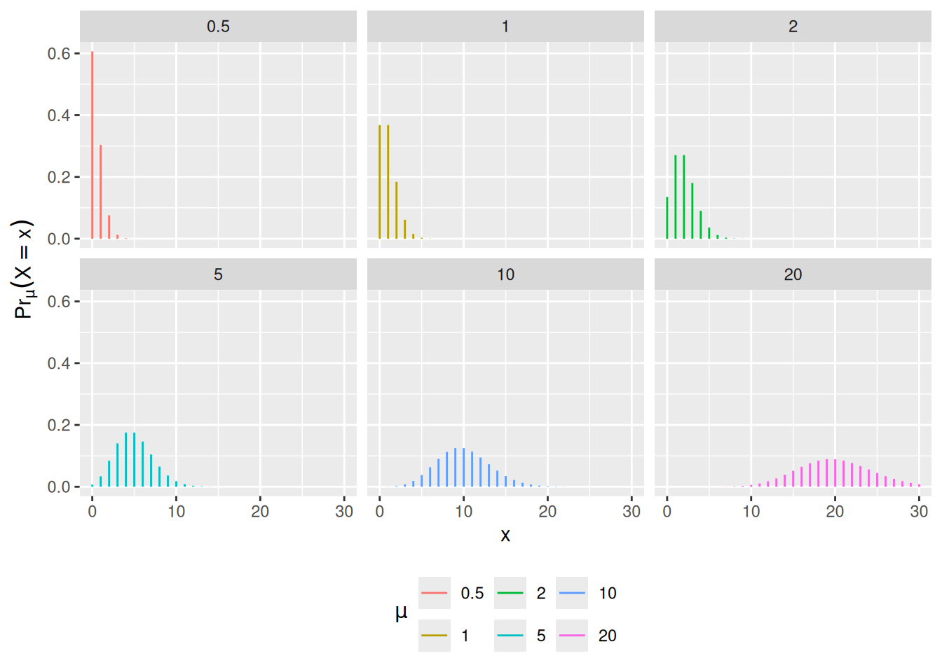
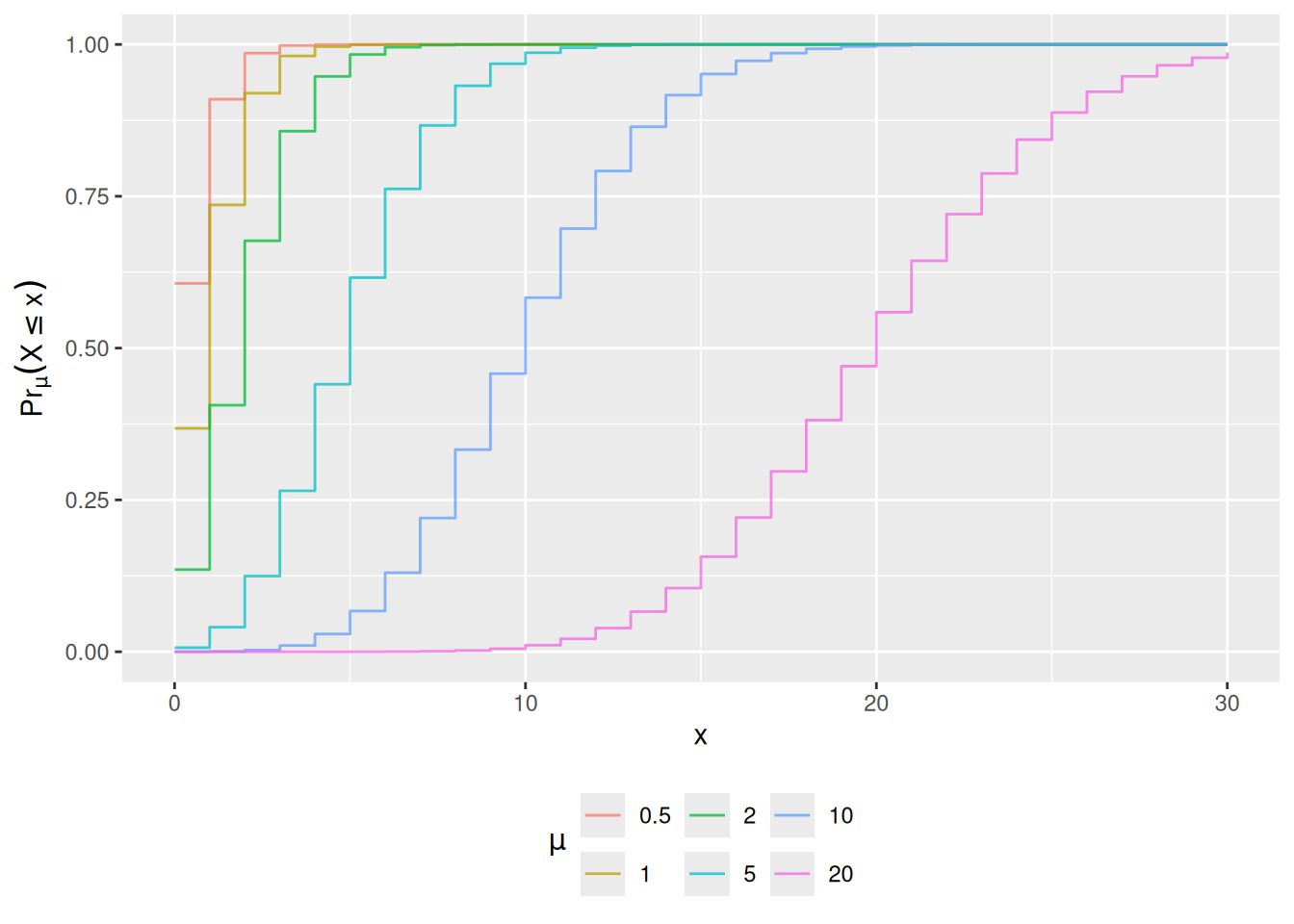
Example 22 (The marginal distribution of the two end elements of a chain of three Gaussian variables)

Example 22 (The marginal distribution of the two end elements of a chain of three Gaussian variables)

Let $\mathord{\smash[b]{\underset{\raise.3ex\hbox{$\scriptstyle\sim$}}{X}}\vphantom{X}}= {(X_1, X_2, X_3)}^{\top}$ be the Gaussian vector of Example 26, with ${\mathbb{E}\mathopen{}\left[\mathord{\smash[b]{\underset{\raise.3ex\hbox{$\scriptstyle\sim$}}{X}}\vphantom{X}}\right]\mathclose{}} = \mathbf{0}$ and

\[ {\operatorname{Var}\mathopen{}\left(\mathord{\smash[b]{\underset{\raise.3ex\hbox{$\scriptstyle\sim$}}{X}}\vphantom{X}}\right)\mathclose{}} = \frac{1}{4} \begin{pmatrix}3 & 2 & 1 \\ 2 & 4 & 2 \\ 1 & 2 & 3\end{pmatrix}. \]

Take $J = \{1, 3\}$. By Theorem 20, keeping the entries in positions 1 and 3,

\[ {(X_1, X_3)}^{\top} \sim \operatorname{N}_2\mathopen{}\left(\mathbf{0}, \frac{1}{4}\begin{pmatrix}3 & 1 \\ 1 & 3\end{pmatrix}\right)\mathclose{}. \]

So $X_1$ and $X_3$ each have variance $3/4$ and covariance $1/4$, and they are not independent, although they are conditionally independent given $X_2$.

Definition 13 (Conditional precision)

Definition 13 (Conditional precision) Let $\mathord{\smash[b]{\underset{\raise.3ex\hbox{$\scriptstyle\sim$}}{X}}\vphantom{X}}$ be a $p \times 1$ multivariate Gaussian vector, and let $\mathord{\smash[b]{\underset{\raise.3ex\hbox{$\scriptstyle\sim$}}{X}}\vphantom{X}}_{-i}$ be $\mathord{\smash[b]{\underset{\raise.3ex\hbox{$\scriptstyle\sim$}}{X}}\vphantom{X}}$ without its $i$th element. The conditional precision of $X_i$ given $\mathord{\smash[b]{\underset{\raise.3ex\hbox{$\scriptstyle\sim$}}{X}}\vphantom{X}}_{-i} = \mathord{\smash[b]{\underset{\raise.3ex\hbox{$\scriptstyle\sim$}}{x}}\vphantom{x}}_{-i}$ is the precision computed from the conditional variance of $X_i$ given $\mathord{\smash[b]{\underset{\raise.3ex\hbox{$\scriptstyle\sim$}}{X}}\vphantom{X}}_{-i} = \mathord{\smash[b]{\underset{\raise.3ex\hbox{$\scriptstyle\sim$}}{x}}\vphantom{x}}_{-i}$:

\[ \tau\mathopen{}\left(X_i \mid \mathord{\smash[b]{\underset{\raise.3ex\hbox{$\scriptstyle\sim$}}{X}}\vphantom{X}}_{-i} = \mathord{\smash[b]{\underset{\raise.3ex\hbox{$\scriptstyle\sim$}}{x}}\vphantom{x}}_{-i}\right)\mathclose{} \stackrel{\text{def}}{=}{\mathopen{}\left({{\operatorname{Var}\mathopen{}\left(X_i \mid\mathord{\smash[b]{\underset{\raise.3ex\hbox{$\scriptstyle\sim$}}{X}}\vphantom{X}}_{-i} = \mathord{\smash[b]{\underset{\raise.3ex\hbox{$\scriptstyle\sim$}}{x}}\vphantom{x}}_{-i}\right)\mathclose{}}}\right)\mathclose{}}^{-1}. \]

Example 23 (The conditional precision of one element of a bivariate Gaussian vector)

Example 23 (The conditional precision of one element of a bivariate Gaussian vector)

Let $\mathord{\smash[b]{\underset{\raise.3ex\hbox{$\scriptstyle\sim$}}{X}}\vphantom{X}}= {(X_1, X_2)}^{\top} \sim \operatorname{N}_2\mathopen{}\left(\mathbf{0}, \begin{pmatrix}1 & \rho \\ \rho & 1\end{pmatrix}\right)\mathclose{}$ with $\mathopen{}\left|\rho\right|\mathclose{} < 1$. By Example 21, $X_1$ given $X_2 = x_2$ has variance $1 - \rho^2$, so the conditional precision of $X_1$ given $X_2 = x_2$ is

\[ \frac{1}{1 - \rho^2}. \]

Definition 14 (Coprecision)

Definition 14 (Coprecision) Let $\mathord{\smash[b]{\underset{\raise.3ex\hbox{$\scriptstyle\sim$}}{X}}\vphantom{X}}$ be a $p \times 1$ multivariate Gaussian vector with $p \ge 2$, let $i \ne j$, and let $\mathord{\smash[b]{\underset{\raise.3ex\hbox{$\scriptstyle\sim$}}{X}}\vphantom{X}}_{-ij}$ be $\mathord{\smash[b]{\underset{\raise.3ex\hbox{$\scriptstyle\sim$}}{X}}\vphantom{X}}$ without its $i$th and $j$th elements. The coprecision of $X_i$ and $X_j$ given $\mathord{\smash[b]{\underset{\raise.3ex\hbox{$\scriptstyle\sim$}}{X}}\vphantom{X}}_{-ij} = \mathord{\smash[b]{\underset{\raise.3ex\hbox{$\scriptstyle\sim$}}{x}}\vphantom{x}}_{-ij}$ is defined through their conditional covariance and their conditional variances as

\[ \frac{-{{\operatorname{Cov}\mathopen{}\left(X_i, X_j \mid\mathord{\smash[b]{\underset{\raise.3ex\hbox{$\scriptstyle\sim$}}{X}}\vphantom{X}}_{-ij} = \mathord{\smash[b]{\underset{\raise.3ex\hbox{$\scriptstyle\sim$}}{x}}\vphantom{x}}_{-ij}\right)\mathclose{}}}} {{{\operatorname{Var}\mathopen{}\left(X_i \mid\mathord{\smash[b]{\underset{\raise.3ex\hbox{$\scriptstyle\sim$}}{X}}\vphantom{X}}_{-ij} = \mathord{\smash[b]{\underset{\raise.3ex\hbox{$\scriptstyle\sim$}}{x}}\vphantom{x}}_{-ij}\right)\mathclose{}}}{{\operatorname{Var}\mathopen{}\left(X_j \mid\mathord{\smash[b]{\underset{\raise.3ex\hbox{$\scriptstyle\sim$}}{X}}\vphantom{X}}_{-ij} = \mathord{\smash[b]{\underset{\raise.3ex\hbox{$\scriptstyle\sim$}}{x}}\vphantom{x}}_{-ij}\right)\mathclose{}}} - \mathopen{}\left({{\operatorname{Cov}\mathopen{}\left(X_i, X_j \mid\mathord{\smash[b]{\underset{\raise.3ex\hbox{$\scriptstyle\sim$}}{X}}\vphantom{X}}_{-ij} = \mathord{\smash[b]{\underset{\raise.3ex\hbox{$\scriptstyle\sim$}}{x}}\vphantom{x}}_{-ij}\right)\mathclose{}}}\right)\mathclose{}^2}. \]

Example 24 (The coprecision of a bivariate Gaussian vector)

Example 24 (The coprecision of a bivariate Gaussian vector)

Let $\mathord{\smash[b]{\underset{\raise.3ex\hbox{$\scriptstyle\sim$}}{X}}\vphantom{X}}= {(X_1, X_2)}^{\top} \sim \operatorname{N}_2\mathopen{}\left(\mathbf{0}, \begin{pmatrix}1 & \rho \\ \rho & 1\end{pmatrix}\right)\mathclose{}$ with $\mathopen{}\left|\rho\right|\mathclose{} < 1$. With no other elements to condition on, the conditional variances of $X_1$ and $X_2$ are both 1 and their conditional covariance is $\rho$, so the coprecision of $X_1$ and $X_2$ is

\[ \frac{-\rho}{1 \cdot 1 - \rho^2} = \frac{-\rho}{1 - \rho^2}. \]

Definition 15 (Precision matrix)

Definition 15 (Precision matrix) Let $\mathord{\smash[b]{\underset{\raise.3ex\hbox{$\scriptstyle\sim$}}{X}}\vphantom{X}}$ be a $p \times 1$ multivariate Gaussian vector. The precision matrix $\tau(\mathord{\smash[b]{\underset{\raise.3ex\hbox{$\scriptstyle\sim$}}{X}}\vphantom{X}})$ of $\mathord{\smash[b]{\underset{\raise.3ex\hbox{$\scriptstyle\sim$}}{X}}\vphantom{X}}$ is the $p \times p$ matrix whose $i$th diagonal element is the conditional precision of $X_i$ given $\mathord{\smash[b]{\underset{\raise.3ex\hbox{$\scriptstyle\sim$}}{X}}\vphantom{X}}_{-i}$, and whose $(i, j)$ element, for $i \ne j$, is the coprecision of $X_i$ and $X_j$ given $\mathord{\smash[b]{\underset{\raise.3ex\hbox{$\scriptstyle\sim$}}{X}}\vphantom{X}}_{-ij}$.

Theorem 21 (The precision matrix is the inverse of the variance matrix)

Theorem 21 (The precision matrix is the inverse of the variance matrix) If $\mathord{\smash[b]{\underset{\raise.3ex\hbox{$\scriptstyle\sim$}}{X}}\vphantom{X}}$ has the multivariate normal distribution $\operatorname{N}_p\mathopen{}\left(\mathord{\smash[b]{\underset{\raise.3ex\hbox{$\scriptstyle\sim$}}{\mu}}\vphantom{\mu}}, \mathbf{\Sigma}\right)\mathclose{}$, then $\tau(\mathord{\smash[b]{\underset{\raise.3ex\hbox{$\scriptstyle\sim$}}{X}}\vphantom{X}}) = {\mathopen{}\left(\mathbf{\Sigma}\right)\mathclose{}}^{-1}$.

Proof

Proof. Let $\mathbf{\Omega} = {\mathopen{}\left(\mathbf{\Sigma}\right)\mathclose{}}^{-1}$. Reordering the elements of $\mathord{\smash[b]{\underset{\raise.3ex\hbox{$\scriptstyle\sim$}}{X}}\vphantom{X}}$ reorders the rows and columns of $\mathbf{\Sigma}$ and of $\mathbf{\Omega}$ in the same way, so for each $i$ and $j$ we may take $X_i$ and $X_j$ to be the last two elements.

Cut $\mathbf{\Sigma}$ into blocks with the first $p - 2$ elements in the first block. By the inverse of a positive definite block matrix, the last $2 \times 2$ block of $\mathbf{\Omega}$ is ${\mathopen{}\left(\mathbf{S}\right)\mathclose{}}^{-1}$, where $\mathbf{S}$ is the Schur complement of the first block of $\mathbf{\Sigma}$. By Theorem 19, $\mathbf{S}$ is the variance matrix of ${(X_i, X_j)}^{\top}$ given $\mathord{\smash[b]{\underset{\raise.3ex\hbox{$\scriptstyle\sim$}}{X}}\vphantom{X}}_{-ij} = \mathord{\smash[b]{\underset{\raise.3ex\hbox{$\scriptstyle\sim$}}{x}}\vphantom{x}}_{-ij}$, so the diagonal elements $v_i$ and $v_j$ of $\mathbf{S}$ are the conditional variances of $X_i$ and $X_j$, and its off-diagonal element $c_{ij}$ is their conditional covariance. The inverse of a $2 \times 2$ matrix gives the off-diagonal element of $\mathbf{\Omega}$:

\[ \begin{aligned} \mathbf{\Omega}_{ij} &= \mathopen{}\left({\mathopen{}\left(\mathbf{S}\right)\mathclose{}}^{-1}\right)\mathclose{}_{12} && \text{(last block of } \mathbf{\Omega} \text{)} \\ &= \frac{-c_{ij}}{v_i v_j - c_{ij}^2} && \text{(inverse of a } 2 \times 2 \text{ matrix)} \end{aligned} \]

which is the coprecision of $X_i$ and $X_j$.

Taking $X_i$ alone as the last element, the last $1 \times 1$ block of $\mathbf{\Omega}$ is ${\mathopen{}\left(\mathbf{S}\right)\mathclose{}}^{-1}$, where by Theorem 19 $\mathbf{S}$ is the conditional variance of $X_i$ given $\mathord{\smash[b]{\underset{\raise.3ex\hbox{$\scriptstyle\sim$}}{X}}\vphantom{X}}_{-i} = \mathord{\smash[b]{\underset{\raise.3ex\hbox{$\scriptstyle\sim$}}{x}}\vphantom{x}}_{-i}$. So $\mathbf{\Omega}_{ii}$ is the inverse of that conditional variance, which is the conditional precision of $X_i$.

Example 25 (The precision matrix of a bivariate Gaussian vector)

Example 25 (The precision matrix of a bivariate Gaussian vector)

Let $\mathord{\smash[b]{\underset{\raise.3ex\hbox{$\scriptstyle\sim$}}{X}}\vphantom{X}}= {(X_1, X_2)}^{\top} \sim \operatorname{N}_2\mathopen{}\left(\mathbf{0}, \begin{pmatrix}1 & \rho \\ \rho & 1\end{pmatrix}\right)\mathclose{}$ with $\mathopen{}\left|\rho\right|\mathclose{} < 1$. By Example 23 and Example 24, the conditional precision of each element is $1 / (1 - \rho^2)$, and the coprecision of $X_1$ and $X_2$ is $-\rho / (1 - \rho^2)$, so

\[ \tau(\mathord{\smash[b]{\underset{\raise.3ex\hbox{$\scriptstyle\sim$}}{X}}\vphantom{X}}) = \frac{1}{1 - \rho^2} \begin{pmatrix}1 & -\rho \\ -\rho & 1\end{pmatrix}. \]

This matrix is the inverse of $\begin{pmatrix}1 & \rho \\ \rho & 1\end{pmatrix}$, as the precision matrix is the inverse of the variance matrix says, because

\[ \begin{aligned} \begin{pmatrix}1 & \rho \\ \rho & 1\end{pmatrix} \cdot \frac{1}{1 - \rho^2} \begin{pmatrix}1 & -\rho \\ -\rho & 1\end{pmatrix} &= \frac{1}{1 - \rho^2} \begin{pmatrix}1 - \rho^2 & -\rho + \rho \\ \rho - \rho & -\rho^2 + 1\end{pmatrix} \\ &= \mathbf{I}_2. \end{aligned} \]

The off-diagonal entries have the opposite sign of $\rho$. Each diagonal entry, $1 / (1 - \rho^2)$, is at least the precision $1 / {\operatorname{Var}\mathopen{}\left(X_1\right)\mathclose{}} = 1$ of $X_1$ alone, and it grows indefinitely as $\mathopen{}\left|\rho\right|\mathclose{} \to 1$. If $\rho = 0$, then $\tau(\mathord{\smash[b]{\underset{\raise.3ex\hbox{$\scriptstyle\sim$}}{X}}\vphantom{X}})$ is the identity matrix, which is diagonal like ${\operatorname{Var}\mathopen{}\left(\mathord{\smash[b]{\underset{\raise.3ex\hbox{$\scriptstyle\sim$}}{X}}\vphantom{X}}\right)\mathclose{}}$ (compare independent components give a diagonal variance matrix).

Theorem 22 (A zero off-diagonal element of the precision matrix means conditional independence)

Theorem 22 (A zero off-diagonal element of the precision matrix means conditional independence) Let $\mathord{\smash[b]{\underset{\raise.3ex\hbox{$\scriptstyle\sim$}}{X}}\vphantom{X}}\sim \operatorname{N}_p\mathopen{}\left(\mathord{\smash[b]{\underset{\raise.3ex\hbox{$\scriptstyle\sim$}}{\mu}}\vphantom{\mu}}, \mathbf{\Sigma}\right)\mathclose{}$ with $p \ge 2$, and let $i \ne j$. The $(i, j)$ element of the precision matrix $\tau(\mathord{\smash[b]{\underset{\raise.3ex\hbox{$\scriptstyle\sim$}}{X}}\vphantom{X}})$ is zero if and only if $X_i$ and $X_j$ are conditionally independent given the continuous random vector $\mathord{\smash[b]{\underset{\raise.3ex\hbox{$\scriptstyle\sim$}}{X}}\vphantom{X}}_{-ij}$, that is, $\mathord{\smash[b]{\underset{\raise.3ex\hbox{$\scriptstyle\sim$}}{X}}\vphantom{X}}$ without its $i$th and $j$th elements.

Proof

Proof. By Theorem 21, the $(i, j)$ element of $\tau(\mathord{\smash[b]{\underset{\raise.3ex\hbox{$\scriptstyle\sim$}}{X}}\vphantom{X}})$ is the coprecision of $X_i$ and $X_j$ given $\mathord{\smash[b]{\underset{\raise.3ex\hbox{$\scriptstyle\sim$}}{X}}\vphantom{X}}_{-ij} = \mathord{\smash[b]{\underset{\raise.3ex\hbox{$\scriptstyle\sim$}}{x}}\vphantom{x}}_{-ij}$. Write $v_i$ and $v_j$ for the conditional variances of $X_i$ and $X_j$ given $\mathord{\smash[b]{\underset{\raise.3ex\hbox{$\scriptstyle\sim$}}{X}}\vphantom{X}}_{-ij} = \mathord{\smash[b]{\underset{\raise.3ex\hbox{$\scriptstyle\sim$}}{x}}\vphantom{x}}_{-ij}$, and $c_{ij}$ for their conditional covariance. By Theorem 19, given $\mathord{\smash[b]{\underset{\raise.3ex\hbox{$\scriptstyle\sim$}}{X}}\vphantom{X}}_{-ij} = \mathord{\smash[b]{\underset{\raise.3ex\hbox{$\scriptstyle\sim$}}{x}}\vphantom{x}}_{-ij}$, ${(X_i, X_j)}^{\top}$ has a bivariate Gaussian distribution whose variance matrix $\mathbf{S}$ is positive definite, with diagonal elements $v_i$ and $v_j$ and off-diagonal element $c_{ij}$, and $\mathbf{S}$ does not depend on $\mathord{\smash[b]{\underset{\raise.3ex\hbox{$\scriptstyle\sim$}}{x}}\vphantom{x}}_{-ij}$. A positive definite matrix has a positive determinant, so $v_i v_j - c_{ij}^2 > 0$, and the coprecision $-c_{ij} / (v_i v_j - c_{ij}^2)$ is zero exactly when $c_{ij} = 0$.

If $c_{ij} = 0$, then $\mathbf{S}$ is diagonal, so by Corollary 7 $X_i$ and $X_j$ are independent given $\mathord{\smash[b]{\underset{\raise.3ex\hbox{$\scriptstyle\sim$}}{X}}\vphantom{X}}_{-ij} = \mathord{\smash[b]{\underset{\raise.3ex\hbox{$\scriptstyle\sim$}}{x}}\vphantom{x}}_{-ij}$, for every $\mathord{\smash[b]{\underset{\raise.3ex\hbox{$\scriptstyle\sim$}}{x}}\vphantom{x}}_{-ij}$. That is, the conditional density of ${(X_i, X_j)}^{\top}$ equals the conditional density of $X_i$ times the conditional density of $X_j$, which is the factorization in the definition of conditional independence. Conversely, if $X_i$ and $X_j$ are conditionally independent, then they are independent given each $\mathord{\smash[b]{\underset{\raise.3ex\hbox{$\scriptstyle\sim$}}{X}}\vphantom{X}}_{-ij} = \mathord{\smash[b]{\underset{\raise.3ex\hbox{$\scriptstyle\sim$}}{x}}\vphantom{x}}_{-ij}$, so by Corollary 7 $c_{ij} = 0$.

Example 26 (A chain of three Gaussian variables)

Example 26 (A chain of three Gaussian variables)

Let $\mathord{\smash[b]{\underset{\raise.3ex\hbox{$\scriptstyle\sim$}}{X}}\vphantom{X}}= {(X_1, X_2, X_3)}^{\top}$ have ${\mathbb{E}\mathopen{}\left[\mathord{\smash[b]{\underset{\raise.3ex\hbox{$\scriptstyle\sim$}}{X}}\vphantom{X}}\right]\mathclose{}} = \mathbf{0}$ and precision matrix

\[ \tau(\mathord{\smash[b]{\underset{\raise.3ex\hbox{$\scriptstyle\sim$}}{X}}\vphantom{X}}) = \begin{pmatrix}2 & -1 & 0 \\ -1 & 2 & -1 \\ 0 & -1 & 2\end{pmatrix}. \]

By Theorem 21, the variance matrix is the inverse of this matrix,

which one can check by multiplying the two matrices to get $\mathbf{I}_3$. So ${\operatorname{Cov}\mathopen{}\left(X_1, X_3\right)\mathclose{}} = 1/4 \ne 0$, and $X_1$ and $X_3$ are not independent. But the $(1, 3)$ element of the precision matrix is 0, so by Theorem 22, $X_1$ and $X_3$ are conditionally independent given $X_2$: once $X_2$ is known, $X_1$ carries no further information about $X_3$.

Theorem 23 (A zero off-diagonal element of the variance matrix means independence)

Theorem 23 (A zero off-diagonal element of the variance matrix means independence) Let $\mathord{\smash[b]{\underset{\raise.3ex\hbox{$\scriptstyle\sim$}}{X}}\vphantom{X}}\sim \operatorname{N}_p\mathopen{}\left(\mathord{\smash[b]{\underset{\raise.3ex\hbox{$\scriptstyle\sim$}}{\mu}}\vphantom{\mu}}, \mathbf{\Sigma}\right)\mathclose{}$ with $p \ge 2$, and let $i \ne j$. The $(i, j)$ element of $\mathbf{\Sigma}$ is zero if and only if $X_i$ and $X_j$ are independent.

Proof

Proof. By Theorem 20, ${(X_i, X_j)}^{\top}$ has a bivariate Gaussian distribution, whose variance matrix has off-diagonal element ${\operatorname{Cov}\mathopen{}\left(X_i, X_j\right)\mathclose{}}$, which by the elements of the variance matrix is the $(i, j)$ element of $\mathbf{\Sigma}$. By Corollary 7 with $p = 2$, $X_i$ and $X_j$ are independent if and only if this element is zero.

Example 27 (Independent but not conditionally independent Gaussian variables)

Example 27 (Independent but not conditionally independent Gaussian variables)

Let $\mathord{\smash[b]{\underset{\raise.3ex\hbox{$\scriptstyle\sim$}}{X}}\vphantom{X}}= {(X_1, X_2, X_3)}^{\top}$ be a Gaussian vector with ${\mathbb{E}\mathopen{}\left[\mathord{\smash[b]{\underset{\raise.3ex\hbox{$\scriptstyle\sim$}}{X}}\vphantom{X}}\right]\mathclose{}} = \mathbf{0}$ and

\[ {\operatorname{Var}\mathopen{}\left(\mathord{\smash[b]{\underset{\raise.3ex\hbox{$\scriptstyle\sim$}}{X}}\vphantom{X}}\right)\mathclose{}} = \begin{pmatrix}1 & 0 & 1/2 \\ 0 & 1 & 1/2 \\ 1/2 & 1/2 & 1\end{pmatrix}. \]

The $(1, 2)$ element is 0, so by Theorem 23, $X_1$ and $X_2$ are independent. By Theorem 21, the precision matrix is the inverse of this matrix,

\[ \tau(\mathord{\smash[b]{\underset{\raise.3ex\hbox{$\scriptstyle\sim$}}{X}}\vphantom{X}}) = \begin{pmatrix}3/2 & 1/2 & -1 \\ 1/2 & 3/2 & -1 \\ -1 & -1 & 2\end{pmatrix}, \]

which one can check by multiplying the two matrices to get $\mathbf{I}_3$. Its $(1, 2)$ element is $1/2 \ne 0$, so by Theorem 22, $X_1$ and $X_2$ are not conditionally independent given $X_3$. So a zero in the variance matrix does not give a zero in the precision matrix. Example 26 shows the reverse case: a zero in the precision matrix, with a nonzero covariance.

Definition 16 (Partial correlation)

Definition 16 (Partial correlation) Let $\mathord{\smash[b]{\underset{\raise.3ex\hbox{$\scriptstyle\sim$}}{X}}\vphantom{X}}$ be a $p \times 1$ multivariate Gaussian vector with $p \ge 2$, let $i \ne j$, and let $\mathord{\smash[b]{\underset{\raise.3ex\hbox{$\scriptstyle\sim$}}{X}}\vphantom{X}}_{-ij}$ be $\mathord{\smash[b]{\underset{\raise.3ex\hbox{$\scriptstyle\sim$}}{X}}\vphantom{X}}$ without its $i$th and $j$th elements. The partial correlation of $X_i$ and $X_j$ given $\mathord{\smash[b]{\underset{\raise.3ex\hbox{$\scriptstyle\sim$}}{X}}\vphantom{X}}_{-ij}$ is their conditional covariance given $\mathord{\smash[b]{\underset{\raise.3ex\hbox{$\scriptstyle\sim$}}{X}}\vphantom{X}}_{-ij} = \mathord{\smash[b]{\underset{\raise.3ex\hbox{$\scriptstyle\sim$}}{x}}\vphantom{x}}_{-ij}$ for a fixed value $\mathord{\smash[b]{\underset{\raise.3ex\hbox{$\scriptstyle\sim$}}{x}}\vphantom{x}}_{-ij}$, divided by the square root of the conditional variance of $X_i$ times that of $X_j$:

\[ \frac{{{\operatorname{Cov}\mathopen{}\left(X_i, X_j \mid\mathord{\smash[b]{\underset{\raise.3ex\hbox{$\scriptstyle\sim$}}{X}}\vphantom{X}}_{-ij} = \mathord{\smash[b]{\underset{\raise.3ex\hbox{$\scriptstyle\sim$}}{x}}\vphantom{x}}_{-ij}\right)\mathclose{}}}} {\sqrt{{{\operatorname{Var}\mathopen{}\left(X_i \mid\mathord{\smash[b]{\underset{\raise.3ex\hbox{$\scriptstyle\sim$}}{X}}\vphantom{X}}_{-ij} = \mathord{\smash[b]{\underset{\raise.3ex\hbox{$\scriptstyle\sim$}}{x}}\vphantom{x}}_{-ij}\right)\mathclose{}}}{{\operatorname{Var}\mathopen{}\left(X_j \mid\mathord{\smash[b]{\underset{\raise.3ex\hbox{$\scriptstyle\sim$}}{X}}\vphantom{X}}_{-ij} = \mathord{\smash[b]{\underset{\raise.3ex\hbox{$\scriptstyle\sim$}}{x}}\vphantom{x}}_{-ij}\right)\mathclose{}}}}}. \]

Theorem 24 (The partial correlation from the precision matrix)

Theorem 24 (The partial correlation from the precision matrix) Let $\mathord{\smash[b]{\underset{\raise.3ex\hbox{$\scriptstyle\sim$}}{X}}\vphantom{X}}\sim \operatorname{N}_p\mathopen{}\left(\mathord{\smash[b]{\underset{\raise.3ex\hbox{$\scriptstyle\sim$}}{\mu}}\vphantom{\mu}}, \mathbf{\Sigma}\right)\mathclose{}$ with $p \ge 2$, and let $i \ne j$. Then the partial correlation of $X_i$ and $X_j$ given $\mathord{\smash[b]{\underset{\raise.3ex\hbox{$\scriptstyle\sim$}}{X}}\vphantom{X}}_{-ij}$ is

\[ \frac{-\tau(\mathord{\smash[b]{\underset{\raise.3ex\hbox{$\scriptstyle\sim$}}{X}}\vphantom{X}})_{ij}}{\sqrt{\tau(\mathord{\smash[b]{\underset{\raise.3ex\hbox{$\scriptstyle\sim$}}{X}}\vphantom{X}})_{ii}\tau(\mathord{\smash[b]{\underset{\raise.3ex\hbox{$\scriptstyle\sim$}}{X}}\vphantom{X}})_{jj}}}, \]

where $\tau(\mathord{\smash[b]{\underset{\raise.3ex\hbox{$\scriptstyle\sim$}}{X}}\vphantom{X}})$ is the precision matrix of $\mathord{\smash[b]{\underset{\raise.3ex\hbox{$\scriptstyle\sim$}}{X}}\vphantom{X}}$.

Proof

Proof. Reordering the elements of $\mathord{\smash[b]{\underset{\raise.3ex\hbox{$\scriptstyle\sim$}}{X}}\vphantom{X}}$ reorders the rows and columns of $\mathbf{\Sigma}$ and of $\tau(\mathord{\smash[b]{\underset{\raise.3ex\hbox{$\scriptstyle\sim$}}{X}}\vphantom{X}})$ in the same way, so we may take $X_i$ and $X_j$ to be the last two elements. Cut $\mathbf{\Sigma}$ into blocks with the first $p - 2$ elements in the first block. By Theorem 21, $\tau(\mathord{\smash[b]{\underset{\raise.3ex\hbox{$\scriptstyle\sim$}}{X}}\vphantom{X}}) = {\mathopen{}\left(\mathbf{\Sigma}\right)\mathclose{}}^{-1}$, and by the inverse of a positive definite block matrix, the last $2 \times 2$ block of $\tau(\mathord{\smash[b]{\underset{\raise.3ex\hbox{$\scriptstyle\sim$}}{X}}\vphantom{X}})$ is ${\mathopen{}\left(\mathbf{S}\right)\mathclose{}}^{-1}$, where $\mathbf{S}$ is the Schur complement of the first block of $\mathbf{\Sigma}$. By Theorem 19, $\mathbf{S}$ is the variance matrix of ${(X_i, X_j)}^{\top}$ given $\mathord{\smash[b]{\underset{\raise.3ex\hbox{$\scriptstyle\sim$}}{X}}\vphantom{X}}_{-ij} = \mathord{\smash[b]{\underset{\raise.3ex\hbox{$\scriptstyle\sim$}}{x}}\vphantom{x}}_{-ij}$, so its diagonal elements $v_i$ and $v_j$ are the conditional variances of $X_i$ and $X_j$, and its off-diagonal element $c_{ij}$ is their conditional covariance. Let $d = v_i v_j - c_{ij}^2$, the determinant of $\mathbf{S}$. The inverse of a $2 \times 2$ matrix gives

\[ {\mathopen{}\left(\mathbf{S}\right)\mathclose{}}^{-1} = \frac{1}{d}\begin{pmatrix}v_j & -c_{ij} \\ -c_{ij} & v_i\end{pmatrix}, \]

so $\tau(\mathord{\smash[b]{\underset{\raise.3ex\hbox{$\scriptstyle\sim$}}{X}}\vphantom{X}})_{ii} = v_j / d$, $\tau(\mathord{\smash[b]{\underset{\raise.3ex\hbox{$\scriptstyle\sim$}}{X}}\vphantom{X}})_{jj} = v_i / d$ and $\tau(\mathord{\smash[b]{\underset{\raise.3ex\hbox{$\scriptstyle\sim$}}{X}}\vphantom{X}})_{ij} = -c_{ij} / d$. Since $\mathbf{S}$ is positive definite, $d > 0$, so

\[ \begin{aligned} \frac{-\tau(\mathord{\smash[b]{\underset{\raise.3ex\hbox{$\scriptstyle\sim$}}{X}}\vphantom{X}})_{ij}}{\sqrt{\tau(\mathord{\smash[b]{\underset{\raise.3ex\hbox{$\scriptstyle\sim$}}{X}}\vphantom{X}})_{ii}\tau(\mathord{\smash[b]{\underset{\raise.3ex\hbox{$\scriptstyle\sim$}}{X}}\vphantom{X}})_{jj}}} &= \frac{c_{ij} / d}{\sqrt{v_i v_j} / d} && \text{(substitute)} \\ &= \frac{c_{ij}}{\sqrt{v_i v_j}}, && \text{(cancel } d > 0 \text{)} \end{aligned} \]

which is the partial correlation of $X_i$ and $X_j$.

Example 28 (The partial correlations of a chain of three Gaussian variables)

Example 28 (The partial correlations of a chain of three Gaussian variables)

Let $\mathord{\smash[b]{\underset{\raise.3ex\hbox{$\scriptstyle\sim$}}{X}}\vphantom{X}}= {(X_1, X_2, X_3)}^{\top}$ be the Gaussian vector of Example 26, with

\[ \tau(\mathord{\smash[b]{\underset{\raise.3ex\hbox{$\scriptstyle\sim$}}{X}}\vphantom{X}}) = \begin{pmatrix}2 & -1 & 0 \\ -1 & 2 & -1 \\ 0 & -1 & 2\end{pmatrix}. \]

By Theorem 24, the partial correlation of $X_1$ and $X_2$ given $X_3$ is

\[ \frac{-\tau(\mathord{\smash[b]{\underset{\raise.3ex\hbox{$\scriptstyle\sim$}}{X}}\vphantom{X}})_{12}}{\sqrt{\tau(\mathord{\smash[b]{\underset{\raise.3ex\hbox{$\scriptstyle\sim$}}{X}}\vphantom{X}})_{11}\tau(\mathord{\smash[b]{\underset{\raise.3ex\hbox{$\scriptstyle\sim$}}{X}}\vphantom{X}})_{22}}} = \frac{1}{\sqrt{2 \cdot 2}} = \frac{1}{2}, \]

and the partial correlation of $X_1$ and $X_3$ given $X_2$ is $-0 / \sqrt{2 \cdot 2} = 0$, as Theorem 22 says for a zero element, although their correlation is not zero.

Theorem 25 (The conditional mean of one element from the precision matrix)

Theorem 25 (The conditional mean of one element from the precision matrix) Let $\mathord{\smash[b]{\underset{\raise.3ex\hbox{$\scriptstyle\sim$}}{X}}\vphantom{X}}\sim \operatorname{N}_p\mathopen{}\left(\mathord{\smash[b]{\underset{\raise.3ex\hbox{$\scriptstyle\sim$}}{\mu}}\vphantom{\mu}}, \mathbf{\Sigma}\right)\mathclose{}$ with $p \ge 2$, let $\mathord{\smash[b]{\underset{\raise.3ex\hbox{$\scriptstyle\sim$}}{X}}\vphantom{X}}_{-i}$ be $\mathord{\smash[b]{\underset{\raise.3ex\hbox{$\scriptstyle\sim$}}{X}}\vphantom{X}}$ without its $i$th element, and let $\mathord{\smash[b]{\underset{\raise.3ex\hbox{$\scriptstyle\sim$}}{x}}\vphantom{x}}_{-i}$ be a fixed value of $\mathord{\smash[b]{\underset{\raise.3ex\hbox{$\scriptstyle\sim$}}{X}}\vphantom{X}}_{-i}$. Then

\[ {{\mathbb{E}\mathopen{}\left[X_i \mid\mathord{\smash[b]{\underset{\raise.3ex\hbox{$\scriptstyle\sim$}}{X}}\vphantom{X}}_{-i} = \mathord{\smash[b]{\underset{\raise.3ex\hbox{$\scriptstyle\sim$}}{x}}\vphantom{x}}_{-i}\right]\mathclose{}}} = \mu_i - \sum_{j \ne i} \frac{\tau(\mathord{\smash[b]{\underset{\raise.3ex\hbox{$\scriptstyle\sim$}}{X}}\vphantom{X}})_{ij}}{\tau(\mathord{\smash[b]{\underset{\raise.3ex\hbox{$\scriptstyle\sim$}}{X}}\vphantom{X}})_{ii}} \mathopen{}\left(x_j - \mu_j\right)\mathclose{}, \]

and ${{\operatorname{Var}\mathopen{}\left(X_i \mid\mathord{\smash[b]{\underset{\raise.3ex\hbox{$\scriptstyle\sim$}}{X}}\vphantom{X}}_{-i} = \mathord{\smash[b]{\underset{\raise.3ex\hbox{$\scriptstyle\sim$}}{x}}\vphantom{x}}_{-i}\right)\mathclose{}}} = 1 / \tau(\mathord{\smash[b]{\underset{\raise.3ex\hbox{$\scriptstyle\sim$}}{X}}\vphantom{X}})_{ii}$, where $\tau(\mathord{\smash[b]{\underset{\raise.3ex\hbox{$\scriptstyle\sim$}}{X}}\vphantom{X}})$ is the precision matrix of $\mathord{\smash[b]{\underset{\raise.3ex\hbox{$\scriptstyle\sim$}}{X}}\vphantom{X}}$.

Proof

Proof. Reordering the elements of $\mathord{\smash[b]{\underset{\raise.3ex\hbox{$\scriptstyle\sim$}}{X}}\vphantom{X}}$ reorders the rows and columns of $\mathbf{\Sigma}$ and of $\tau(\mathord{\smash[b]{\underset{\raise.3ex\hbox{$\scriptstyle\sim$}}{X}}\vphantom{X}})$ in the same way, so we may take $X_i$ to be the last element. Cut $\mathord{\smash[b]{\underset{\raise.3ex\hbox{$\scriptstyle\sim$}}{X}}\vphantom{X}}$, $\mathord{\smash[b]{\underset{\raise.3ex\hbox{$\scriptstyle\sim$}}{\mu}}\vphantom{\mu}}$ and $\mathbf{\Sigma}$ into blocks with $\mathord{\smash[b]{\underset{\raise.3ex\hbox{$\scriptstyle\sim$}}{X}}\vphantom{X}}_{-i}$ first and $X_i$ last, as in Theorem 19 with $\mathord{\smash[b]{\underset{\raise.3ex\hbox{$\scriptstyle\sim$}}{X}}\vphantom{X}}_1 = \mathord{\smash[b]{\underset{\raise.3ex\hbox{$\scriptstyle\sim$}}{X}}\vphantom{X}}_{-i}$ and $\mathord{\smash[b]{\underset{\raise.3ex\hbox{$\scriptstyle\sim$}}{X}}\vphantom{X}}_2 = X_i$, and let $\mathbf{S} = \mathbf{\Sigma}_{22} - \mathbf{\Sigma}_{21}{\mathopen{}\left(\mathbf{\Sigma}_{11}\right)\mathclose{}}^{-1}\mathbf{\Sigma}_{12}$. By Theorem 19, the conditional mean and conditional variance of $X_i$ given $\mathord{\smash[b]{\underset{\raise.3ex\hbox{$\scriptstyle\sim$}}{X}}\vphantom{X}}_{-i} = \mathord{\smash[b]{\underset{\raise.3ex\hbox{$\scriptstyle\sim$}}{x}}\vphantom{x}}_{-i}$ are

\[ \mu_i + \mathbf{\Sigma}_{21}{\mathopen{}\left(\mathbf{\Sigma}_{11}\right)\mathclose{}}^{-1}\mathopen{}\left(\mathord{\smash[b]{\underset{\raise.3ex\hbox{$\scriptstyle\sim$}}{x}}\vphantom{x}}_{-i} - \mathord{\smash[b]{\underset{\raise.3ex\hbox{$\scriptstyle\sim$}}{\mu}}\vphantom{\mu}}_{-i}\right)\mathclose{} \quad \text{and} \quad \mathbf{S}. \]

By Theorem 21, $\tau(\mathord{\smash[b]{\underset{\raise.3ex\hbox{$\scriptstyle\sim$}}{X}}\vphantom{X}}) = {\mathopen{}\left(\mathbf{\Sigma}\right)\mathclose{}}^{-1}$, and by the inverse of a positive definite block matrix, its blocks $\mathbf{\Omega}_{21}$ and $\mathbf{\Omega}_{22}$ satisfy

Here $\mathbf{\Omega}_{22} = \tau(\mathord{\smash[b]{\underset{\raise.3ex\hbox{$\scriptstyle\sim$}}{X}}\vphantom{X}})_{ii}$ is a scalar, so the conditional variance is $\mathbf{S} = 1 / \tau(\mathord{\smash[b]{\underset{\raise.3ex\hbox{$\scriptstyle\sim$}}{X}}\vphantom{X}})_{ii}$, and multiplying the second equation by $\mathbf{S}$ gives

\[ \begin{aligned} \mathbf{\Sigma}_{21}{\mathopen{}\left(\mathbf{\Sigma}_{11}\right)\mathclose{}}^{-1} &= -\mathbf{S}\mathbf{\Omega}_{21} && \text{(multiply by } \mathbf{S} \text{)} \\ &= -\frac{\mathbf{\Omega}_{21}}{\tau(\mathord{\smash[b]{\underset{\raise.3ex\hbox{$\scriptstyle\sim$}}{X}}\vphantom{X}})_{ii}}. && \text{(} \mathbf{S} = 1 / \tau(\mathord{\smash[b]{\underset{\raise.3ex\hbox{$\scriptstyle\sim$}}{X}}\vphantom{X}})_{ii} \text{)} \end{aligned} \]

The elements of $\mathbf{\Omega}_{21}$ are $\tau(\mathord{\smash[b]{\underset{\raise.3ex\hbox{$\scriptstyle\sim$}}{X}}\vphantom{X}})_{ij}$ for $j \ne i$, so the conditional mean is

\[ \mu_i - \sum_{j \ne i} \frac{\tau(\mathord{\smash[b]{\underset{\raise.3ex\hbox{$\scriptstyle\sim$}}{X}}\vphantom{X}})_{ij}}{\tau(\mathord{\smash[b]{\underset{\raise.3ex\hbox{$\scriptstyle\sim$}}{X}}\vphantom{X}})_{ii}} \mathopen{}\left(x_j - \mu_j\right)\mathclose{}. \]

Example 29 (The conditional mean and variance of the middle element of a chain of three Gaussian variables)

Example 29 (The conditional mean and variance of the middle element of a chain of three Gaussian variables)

\[ \tau(\mathord{\smash[b]{\underset{\raise.3ex\hbox{$\scriptstyle\sim$}}{X}}\vphantom{X}}) = \begin{pmatrix}2 & -1 & 0 \\ -1 & 2 & -1 \\ 0 & -1 & 2\end{pmatrix}. \]

By Theorem 25 with $i = 2$, using the second row of the precision matrix,

\[ {{\mathbb{E}\mathopen{}\left[X_2 \mid X_1 = x_1, X_3 = x_3\right]\mathclose{}}} = -\frac{-1}{2}x_1 - \frac{-1}{2}x_3 = \frac{x_1 + x_3}{2}, \]

and ${{\operatorname{Var}\mathopen{}\left(X_2 \mid X_1 = x_1, X_3 = x_3\right)\mathclose{}}} = 1 / 2$. So the conditional mean of $X_2$ is the midpoint of its two neighbors’ values. The coefficient of $x_1$ is $-\tau(\mathord{\smash[b]{\underset{\raise.3ex\hbox{$\scriptstyle\sim$}}{X}}\vphantom{X}})_{21} / \tau(\mathord{\smash[b]{\underset{\raise.3ex\hbox{$\scriptstyle\sim$}}{X}}\vphantom{X}})_{22} = 1/2$, and the coefficient of a neighbor with a zero off-diagonal element would be zero, as Theorem 22 says.

Theorem 26 (Mahalanobis distance in eigenvector coordinates)

Theorem 26 (Mahalanobis distance in eigenvector coordinates) Let $\mathbf{\Sigma}$ be positive definite, with eigendecomposition $\mathbf{\Sigma} = \mathbf{Q}\mathbf{\Lambda}{\mathbf{Q}}^{\top}$, where $\mathbf{Q}$ has columns $\mathord{\smash[b]{\underset{\raise.3ex\hbox{$\scriptstyle\sim$}}{q}}\vphantom{q}}_1, \ldots, \mathord{\smash[b]{\underset{\raise.3ex\hbox{$\scriptstyle\sim$}}{q}}\vphantom{q}}_p$ and $\mathbf{\Lambda}$ has diagonal elements $\lambda_1, \ldots, \lambda_p$. Then:

\[ \Delta(\mathord{\smash[b]{\underset{\raise.3ex\hbox{$\scriptstyle\sim$}}{x}}\vphantom{x}})^2 = \sum_{i=1}^p\frac{\mathopen{}\left({\mathord{\smash[b]{\underset{\raise.3ex\hbox{$\scriptstyle\sim$}}{q}}\vphantom{q}}_i}^{\top}(\mathord{\smash[b]{\underset{\raise.3ex\hbox{$\scriptstyle\sim$}}{x}}\vphantom{x}}- \mathord{\smash[b]{\underset{\raise.3ex\hbox{$\scriptstyle\sim$}}{\mu}}\vphantom{\mu}})\right)\mathclose{}^2}{\lambda_i} \]

Proof

Proof. Let $\mathord{\smash[b]{\underset{\raise.3ex\hbox{$\scriptstyle\sim$}}{y}}\vphantom{y}} = {\mathbf{Q}}^{\top}(\mathord{\smash[b]{\underset{\raise.3ex\hbox{$\scriptstyle\sim$}}{x}}\vphantom{x}}- \mathord{\smash[b]{\underset{\raise.3ex\hbox{$\scriptstyle\sim$}}{\mu}}\vphantom{\mu}})$, whose $i$-th element is $y_i = {\mathord{\smash[b]{\underset{\raise.3ex\hbox{$\scriptstyle\sim$}}{q}}\vphantom{q}}_i}^{\top}(\mathord{\smash[b]{\underset{\raise.3ex\hbox{$\scriptstyle\sim$}}{x}}\vphantom{x}}- \mathord{\smash[b]{\underset{\raise.3ex\hbox{$\scriptstyle\sim$}}{\mu}}\vphantom{\mu}})$. By the inverse of a positive definite matrix, $\mathbf{\Sigma}^{-1} = \mathbf{Q}\mathbf{\Lambda}^{-1}{\mathbf{Q}}^{\top}$, with every $\lambda_i > 0$. So:

\[ \begin{aligned} \Delta(\mathord{\smash[b]{\underset{\raise.3ex\hbox{$\scriptstyle\sim$}}{x}}\vphantom{x}})^2 &= {(\mathord{\smash[b]{\underset{\raise.3ex\hbox{$\scriptstyle\sim$}}{x}}\vphantom{x}}- \mathord{\smash[b]{\underset{\raise.3ex\hbox{$\scriptstyle\sim$}}{\mu}}\vphantom{\mu}})}^{\top} \mathbf{Q}\mathbf{\Lambda}^{-1}{\mathbf{Q}}^{\top} (\mathord{\smash[b]{\underset{\raise.3ex\hbox{$\scriptstyle\sim$}}{x}}\vphantom{x}}- \mathord{\smash[b]{\underset{\raise.3ex\hbox{$\scriptstyle\sim$}}{\mu}}\vphantom{\mu}}) && \text{(definition; substitute } \mathbf{\Sigma}^{-1} \text{)} \\ &= {\mathord{\smash[b]{\underset{\raise.3ex\hbox{$\scriptstyle\sim$}}{y}}\vphantom{y}}}^{\top} \mathbf{\Lambda}^{-1} \mathord{\smash[b]{\underset{\raise.3ex\hbox{$\scriptstyle\sim$}}{y}}\vphantom{y}} && \text{(} {(\mathord{\smash[b]{\underset{\raise.3ex\hbox{$\scriptstyle\sim$}}{x}}\vphantom{x}}- \mathord{\smash[b]{\underset{\raise.3ex\hbox{$\scriptstyle\sim$}}{\mu}}\vphantom{\mu}})}^{\top}\mathbf{Q} = {\mathord{\smash[b]{\underset{\raise.3ex\hbox{$\scriptstyle\sim$}}{y}}\vphantom{y}}}^{\top} \text{)} \\ &= \sum_{i=1}^p\frac{y_i^2}{\lambda_i} && \text{(} \mathbf{\Lambda}^{-1} \text{ is diagonal)} \end{aligned} \]

Remark

Remark. $y_i$ is the coordinate of $\mathord{\smash[b]{\underset{\raise.3ex\hbox{$\scriptstyle\sim$}}{x}}\vphantom{x}}- \mathord{\smash[b]{\underset{\raise.3ex\hbox{$\scriptstyle\sim$}}{\mu}}\vphantom{\mu}}$ along the eigenvector $\mathord{\smash[b]{\underset{\raise.3ex\hbox{$\scriptstyle\sim$}}{q}}\vphantom{q}}_i$. So the set of points at Mahalanobis distance $\delta$ from $\mathord{\smash[b]{\underset{\raise.3ex\hbox{$\scriptstyle\sim$}}{\mu}}\vphantom{\mu}}$, where the multivariate normal density is constant (Corollary 6), is an ellipse ($p = 2$) or ellipsoid centered at $\mathord{\smash[b]{\underset{\raise.3ex\hbox{$\scriptstyle\sim$}}{\mu}}\vphantom{\mu}}$, with axes along the eigenvectors of $\mathbf{\Sigma}$ and half-length $\delta\sqrt{\lambda_i}$ along $\mathord{\smash[b]{\underset{\raise.3ex\hbox{$\scriptstyle\sim$}}{q}}\vphantom{q}}_i$.

Example 30 (Elliptical contours of a bivariate normal density)

Example 30 (Elliptical contours of a bivariate normal density) Let $\mathord{\smash[b]{\underset{\raise.3ex\hbox{$\scriptstyle\sim$}}{\mu}}\vphantom{\mu}} = \mathord{\smash[b]{\underset{\raise.3ex\hbox{$\scriptstyle\sim$}}{0}}\vphantom{0}}$ and $\mathbf{\Sigma} = \begin{pmatrix}2 & 1 \\ 1 & 2\end{pmatrix}$, which has eigenvalues $3$ and $1$, with eigenvectors $\mathord{\smash[b]{\underset{\raise.3ex\hbox{$\scriptstyle\sim$}}{q}}\vphantom{q}}_1 = \frac{1}{\sqrt{2}}{(1, 1)}^{\top}$ and $\mathord{\smash[b]{\underset{\raise.3ex\hbox{$\scriptstyle\sim$}}{q}}\vphantom{q}}_2 = \frac{1}{\sqrt{2}}{(1, -1)}^{\top}$ (an eigendecomposition example). By Theorem 26:

\[ \Delta(\mathord{\smash[b]{\underset{\raise.3ex\hbox{$\scriptstyle\sim$}}{x}}\vphantom{x}})^2 = \frac{(x_1 + x_2)^2}{2 \cdot 3} + \frac{(x_1 - x_2)^2}{2 \cdot 1} \]

The point

\[ \begin{aligned} \mathord{\smash[b]{\underset{\raise.3ex\hbox{$\scriptstyle\sim$}}{x}}\vphantom{x}}&= \sqrt{3}\,\mathord{\smash[b]{\underset{\raise.3ex\hbox{$\scriptstyle\sim$}}{q}}\vphantom{q}}_1 \\ &= \sqrt{3/2}\,{(1, 1)}^{\top} \end{aligned} \]

has $x_1 + x_2 = \sqrt{6}$ and $x_1 - x_2 = 0$, so

\[ \begin{aligned} \Delta(\mathord{\smash[b]{\underset{\raise.3ex\hbox{$\scriptstyle\sim$}}{x}}\vphantom{x}})^2 &= 6/6 \\ &= 1; \end{aligned} \]

the point $\mathord{\smash[b]{\underset{\raise.3ex\hbox{$\scriptstyle\sim$}}{x}}\vphantom{x}}= \mathord{\smash[b]{\underset{\raise.3ex\hbox{$\scriptstyle\sim$}}{q}}\vphantom{q}}_2$ has $x_1 + x_2 = 0$ and $x_1 - x_2 = \sqrt{2}$, so

\[ \begin{aligned} \Delta(\mathord{\smash[b]{\underset{\raise.3ex\hbox{$\scriptstyle\sim$}}{x}}\vphantom{x}})^2 &= 2/2 \\ &= 1. \end{aligned} \]

So the contour $\Delta(\mathord{\smash[b]{\underset{\raise.3ex\hbox{$\scriptstyle\sim$}}{x}}\vphantom{x}}) = 1$ of the $\operatorname{N}_2\mathopen{}\left(\mathord{\smash[b]{\underset{\raise.3ex\hbox{$\scriptstyle\sim$}}{0}}\vphantom{0}}, \mathbf{\Sigma}\right)\mathclose{}$ density is an ellipse stretched along ${(1, 1)}^{\top}$, with half-length $\sqrt{3}$, and squeezed along ${(1, -1)}^{\top}$, with half-length $1$: $X_1$ and $X_2$ are positively correlated (Figure 6).

Show code

# The covariance matrix of the example and its eigendecomposition.
mh_entries <- c(2, 1, 1, 2)
mh_covmat <- matrix(mh_entries, nrow = 2)
mh_eig <- eigen(mh_covmat)
mh_values <- mh_eig$values
mh_expected <- c(3, 1)
mh_matches <- all.equal(mh_values, mh_expected)
stopifnot(mh_matches)

# The Mahalanobis distance of each grid point from the mean zero.
mh_axis <- seq(-3.5, 3.5, length.out = 200)
mh_grid <- tidyr::expand_grid(x1 = mh_axis, x2 = mh_axis)
mh_points <- as.matrix(mh_grid)
mh_inverse <- solve(mh_covmat)
mh_quad <- (mh_points %*% mh_inverse) * mh_points
mh_sums <- rowSums(mh_quad)
mh_dist <- sqrt(mh_sums)
mh_grid <- dplyr::mutate(mh_grid, mahal = mh_dist)

# The points of the example: sqrt(3) q1 and q2, each at distance 1.
mh_long <- sqrt(3 / 2)
mh_short <- 1 / sqrt(2)
mh_marks_x1 <- c(mh_long, mh_short)
mh_marks_x2 <- c(mh_long, -mh_short)
mh_marks <- tibble::tibble(x1 = mh_marks_x1, x2 = mh_marks_x2)

mh_contour_aes <- ggplot2::aes(z = mahal, colour = ggplot2::after_stat(level))
mh_breaks <- c(1, 2)
mh_contours <- ggplot2::geom_contour(mh_contour_aes, breaks = mh_breaks)
mh_dots <- ggplot2::geom_point(data = mh_marks, size = 2.5)
mh_colours <- ggplot2::scale_colour_viridis_c(
  name = "Mahalanobis distance",
  end = 0.7,
  breaks = mh_breaks,
  guide = "legend"
)
mh_plot <- mh_grid |>
  ggplot2::ggplot() +
  ggplot2::aes(x1, x2) +
  mh_contours +
  mh_dots +
  mh_colours +
  ggplot2::coord_fixed(expand = FALSE) +
  ggplot2::labs(x = "x1", y = "x2") +
  ggplot2::theme(legend.position = "bottom")

mh_is_html <- knitr::is_html_output()
if (mh_is_html) {
  mh_legend <- list(
    orientation = "h",
    x = 0.5,
    xanchor = "center",
    y = -0.25
  )
  mh_widget <- plotly::ggplotly(mh_plot) |>
    plotly::layout(legend = mh_legend) |>
    plotly::config(displaylogo = FALSE, responsive = TRUE)
  htmltools::div(
    role = "img",
    `aria-label` = fig_alt_mahal_eigen,
    mh_widget
  )
} else {
  mh_plot
}

Figure 6: The contours of the Mahalanobis distance at $1$ and $2$ for the example. The dots are the points $\sqrt{3}\,\mathord{\smash[b]{\underset{\raise.3ex\hbox{$\scriptstyle\sim$}}{q}}\vphantom{q}}_1$ and $\mathord{\smash[b]{\underset{\raise.3ex\hbox{$\scriptstyle\sim$}}{q}}\vphantom{q}}_2$ of the example on the inner ellipse.

Show code

mh3_entries <- c(2, 1, 1, 2)
mh3_covmat <- matrix(mh3_entries, nrow = 2)
mh3_inverse <- solve(mh3_covmat)
mh3_x1 <- seq(-3.5, 3.5, length.out = 101)
mh3_x2 <- seq(-3.5, 3.5, length.out = 101)
mh3_grid <- tidyr::expand_grid(x1 = mh3_x1, x2 = mh3_x2)
mh3_points <- as.matrix(mh3_grid)
mh3_quad <- (mh3_points %*% mh3_inverse) * mh3_points
mh3_sums <- rowSums(mh3_quad)
mh3_dist <- sqrt(mh3_sums)
mh3_n_x2 <- length(mh3_x2)
mh3_z <- matrix(mh3_dist, nrow = mh3_n_x2)

# The points of the example: sqrt(3) q1 and q2, each at distance 1.
mh3_long <- sqrt(3 / 2)
mh3_short <- 1 / sqrt(2)
mh3_marks_x1 <- c(mh3_long, mh3_short)
mh3_marks_x2 <- c(mh3_long, -mh3_short)
mh3_marks_z <- c(1, 1)
mh3_marks <- tibble::tibble(
  x1 = mh3_marks_x1,
  x2 = mh3_marks_x2,
  z = mh3_marks_z
)
mh3_marker <- list(color = "black", size = 5)
mh3_contours_z <- list(
  show = TRUE,
  start = 1,
  end = 2,
  size = 1,
  color = "red"
)
mh3_contours <- list(z = mh3_contours_z)
mh3_stops <- c(0, 1)
mh3_cols <- c("#CCE0F0", "#0072B2")
mh3_scale <- list(mh3_stops, mh3_cols)
mh3_eye <- list(x = 1.6, y = -1.6, z = 0.9)
mh3_camera <- list(eye = mh3_eye)
mh3_xaxis <- list(title = "x1")
mh3_yaxis <- list(title = "x2")
mh3_zaxis <- list(title = "Mahalanobis distance")
mh3_scene <- list(
  xaxis = mh3_xaxis,
  yaxis = mh3_yaxis,
  zaxis = mh3_zaxis,
  camera = mh3_camera
)
mh3_widget <- plotly::plot_ly() |>
  plotly::add_surface(
    x = mh3_x1,
    y = mh3_x2,
    z = mh3_z,
    contours = mh3_contours,
    colorscale = mh3_scale,
    showscale = FALSE,
    opacity = 0.8
  ) |>
  plotly::add_markers(
    data = mh3_marks,
    x = ~x1,
    y = ~x2,
    z = ~z,
    showlegend = FALSE,
    marker = mh3_marker
  ) |>
  plotly::layout(scene = mh3_scene)
htmltools::div(
  role = "img",
  `aria-label` = fig_alt_mahal_surf,
  mh3_widget
)

Figure 7: The Mahalanobis distance is a surface over the plane, a cone whose horizontal slices are the ellipses of Figure 6. The red lines are the contours at $1$ and $2$, and the dots are the points $\sqrt{3}\,\mathord{\smash[b]{\underset{\raise.3ex\hbox{$\scriptstyle\sim$}}{q}}\vphantom{q}}_1$ and $\mathord{\smash[b]{\underset{\raise.3ex\hbox{$\scriptstyle\sim$}}{q}}\vphantom{q}}_2$ of the example on the inner one.

Theorem 27 (The maximum of the Gaussian density)

Theorem 27 (The maximum of the Gaussian density) If $X \sim {\operatorname{N}\mathopen{}\left(\mu, \sigma^2\right)\mathclose{}}$ (Gaussian distribution), then its density is largest at $x = \mu$, where it equals:

\[\max_x \mathbb{p}(X=x) = \frac{1}{\sigma\sqrt{2\pi}}\]

Proof

Proof. For each $x \in \mathbb{R}$, the quantity $u(x) \stackrel{\text{def}}{=}(x-\mu)^2 / (2\sigma^2)$ is at least $0$, and it equals $0$ only at $x = \mu$. The factor $\text{e}^{-u(x)}$ of the density is at most $1$:

\[ \begin{aligned} -u(x) &\le 0 && \text{(a square is non-negative, and } 2\sigma^2> 0 \text{)} \\ \text{e}^{-u(x)} &\le \text{e}^{0} && \text{(} \text{e}^t \text{ is increasing in } t \text{)} \\ &= 1 && \text{(} \text{e}^0 = 1 \text{)} \end{aligned} \]

Multiplying both sides by $1 / (\sigma\sqrt{2\pi}) > 0$ keeps their order:

\[ \begin{aligned} \mathbb{p}(X=x) &= \frac{1}{\sigma\sqrt{2\pi}} \text{e}^{-u(x)} && \text{(Gaussian density)} \\ &\le \frac{1}{\sigma\sqrt{2\pi}} && \text{(} \text{e}^{-u(x)} \le 1 \text{)} \end{aligned} \]

Equality holds at $x = \mu$, where $u(x) = 0$, so the density peaks there.

Example 31 (The peak of the Gaussian density grows as the standard deviation shrinks)

Example 31 (The peak of the Gaussian density grows as the standard deviation shrinks) By Theorem 27, the peak of the density of ${\operatorname{N}\mathopen{}\left(0, \sigma^2\right)\mathclose{}}$ is $1 / (\sigma\sqrt{2\pi})$. Figure 8 marks each peak for standard deviations $0.5$, $1$ and $2$.

Show code

sds <- c(0.5, 1, 2)
x_grid <- seq(-6, 6, length.out = 400)
sd_label <- latex2exp::TeX("$\\sigma$")
density_label <- latex2exp::TeX("$f(x)$")

normal_curves <-
  dplyr::tibble(sd = sds) |>
  dplyr::reframe(.by = sd, x = x_grid) |>
  dplyr::mutate(
    density = dnorm(x, mean = 0, sd = sd),
    sd = factor(sd)
  )

normal_peaks <-
  dplyr::tibble(sd = sds) |>
  dplyr::mutate(
    peak = 1 / (sd * sqrt(2 * pi)),
    sd = factor(sd)
  )

normal_plot <-
  normal_curves |>
  ggplot2::ggplot() +
  ggplot2::aes(x = x, y = density, col = sd) +
  ggplot2::geom_line() +
  ggplot2::geom_point(
    data = normal_peaks,
    ggplot2::aes(x = 0, y = peak)
  ) +
  ggplot2::labs(col = sd_label, y = density_label) +
  ggplot2::theme(legend.position = "bottom")

print(normal_plot)

Three Gaussian curves; narrower ones peak higher. — Figure 8: Gaussian densities, with each peak marked

As $\sigma \to 0$, the peak $1 / (\sigma\sqrt{2\pi})$ grows indefinitely, so a density can exceed $1$.

Theorem 28 (Gaussian distributions are closed under affine transformations)

Theorem 28 (Gaussian distributions are closed under affine transformations) If $X \sim {\operatorname{N}\mathopen{}\left(\mu, \sigma^2\right)\mathclose{}}$ and $a \ne 0$, then $aX + b \sim {\operatorname{N}\mathopen{}\left(a\mu+ b, a^2\sigma^2\right)\mathclose{}}$.

Proof

Proof. Let $Y = aX + b$. Let $f$ be the density of $X$. The CDF of $Y$ is $\mathbb{F}_Y\mathopen{}\left(y\right)\mathclose{} = \Pr(aX + b \le y)$. The density $f$ is continuous everywhere. So at every $y$, the derivative of $\mathbb{F}_Y\mathopen{}\left(y\right)\mathclose{}$ is the density of $Y$, by the derivative of the CDF is the density. To differentiate $\mathbb{F}_Y\mathopen{}\left(y\right)\mathclose{}$, write it through the CDF $\mathbb{F}_X$ of $X$. There are two cases, by the sign of $a$.

Case $a > 0$. Dividing by $a > 0$ leaves $\le$ as $\le$, so:

\[ \begin{aligned} \mathbb{F}_Y\mathopen{}\left(y\right)\mathclose{} &= {\Pr\mathopen{}\left(X \le \frac{y-b}{a}\right)\mathclose{}} && \text{(} aX + b \le y \iff X \le (y-b)/a \text{)} \\ &= \mathbb{F}_X\mathopen{}\left(\frac{y-b}{a}\right)\mathclose{} && \text{(definition of the CDF)} \end{aligned} \]

The chain rule gives the derivative:

\[ \frac{\partial}{\partial y} \mathbb{F}_Y\mathopen{}\left(y\right)\mathclose{} = \frac{1}{a} f\mathopen{}\left(\frac{y-b}{a}\right)\mathclose{} = \frac{1}{\mathopen{}\left|a\right|\mathclose{}} f\mathopen{}\left(\frac{y-b}{a}\right)\mathclose{} \quad \text{(} \mathopen{}\left|a\right|\mathclose{} = a \text{)} \]
Case $a < 0$. Dividing by $a < 0$ turns $\le$ into $\ge$, and $\Pr(X = x) = 0$ for a continuous random variable $X$, so:

\[ \begin{aligned} \mathbb{F}_Y\mathopen{}\left(y\right)\mathclose{} &= {\Pr\mathopen{}\left(X \ge \frac{y-b}{a}\right)\mathclose{}} && \text{(} aX + b \le y \iff X \ge (y-b)/a \text{)} \\ &= 1 - \mathbb{F}_X\mathopen{}\left(\frac{y-b}{a}\right)\mathclose{} && \text{(complement, and } \Pr(X = (y-b)/a) = 0 \text{)} \end{aligned} \]

The chain rule gives the derivative:

\[ \frac{\partial}{\partial y} \mathbb{F}_Y\mathopen{}\left(y\right)\mathclose{} = -\frac{1}{a} f\mathopen{}\left(\frac{y-b}{a}\right)\mathclose{} = \frac{1}{\mathopen{}\left|a\right|\mathclose{}} f\mathopen{}\left(\frac{y-b}{a}\right)\mathclose{} \quad \text{(} \mathopen{}\left|a\right|\mathclose{} = -a \text{)} \]

In both cases, $Y$ has density $\mathbb{p}(Y=y) = f\mathopen{}\left((y-b)/a\right)\mathclose{} / \mathopen{}\left|a\right|\mathclose{}$. Substitute the Gaussian density of $X$:

\[ \begin{aligned} \mathbb{p}(Y=y) &= \frac{1}{\mathopen{}\left|a\right|\mathclose{}} \cdot\frac{1}{\sigma\sqrt{2\pi}} \text{e}^{-\frac{\mathopen{}\left((y-b)/a - \mu\right)\mathclose{}^2}{2\sigma^2}} && \text{(Gaussian density of } X \text{)} \\ &= \frac{1}{\mathopen{}\left|a\right|\mathclose{}\sigma\sqrt{2\pi}} \text{e}^{-\frac{\mathopen{}\left((y-b-a\mu)/a\right)\mathclose{}^2}{2\sigma^2}} && \text{(common denominator } a \text{)} \\ &= \frac{1}{\mathopen{}\left|a\right|\mathclose{}\sigma\sqrt{2\pi}} \text{e}^{-\frac{(y-(a\mu+b))^2}{2a^2\sigma^2}} && \text{(} (u/a)^2 = u^2/a^2 \text{)} \\ &= \frac{1}{\sqrt{a^2\sigma^2}\sqrt{2\pi}} \text{e}^{-\frac{(y-(a\mu+b))^2}{2a^2\sigma^2}} && \text{(} \mathopen{}\left|a\right|\mathclose{}\sigma= \sqrt{a^2\sigma^2} \text{)} \end{aligned} \]

The last line is the density of ${\operatorname{N}\mathopen{}\left(a\mu+ b, a^2\sigma^2\right)\mathclose{}}$ because $a^2\sigma^2> 0$.

Example 32 (Standardizing a Gaussian random variable)

Example 32 (Standardizing a Gaussian random variable)

Let $X \sim {\operatorname{N}\mathopen{}\left(\mu, \sigma^2\right)\mathclose{}}$ with $\sigma> 0$, and let $Z = (X - \mu) / \sigma$. Then $Z = aX + b$ with $a = 1 / \sigma$ and $b = -\mu/ \sigma$, and $a \ne 0$. By Theorem 28, $Z$ is Gaussian with parameters:

\[ \begin{aligned} a\mu+ b &= \frac{\mu}{\sigma} - \frac{\mu}{\sigma} && \text{(substitute } a \text{ and } b \text{)} \\ &= 0 && \text{(} u - u = 0 \text{)} \\ a^2\sigma^2 &= \frac{\sigma^2}{\sigma^2} && \text{(} a^2 = 1/\sigma^2\text{)} \\ &= 1 && \text{(} u/u = 1 \text{)} \end{aligned} \]

So $Z \sim {\operatorname{N}\mathopen{}\left(0, 1\right)\mathclose{}}$.

9 Mixture distributions

Definition 17 (Mixture density)

Definition 17 (Mixture density) Let ${\mathbb{p}_1}, \ldots, {\mathbb{p}_K}$ be densities on $\mathbb{R}$, and let $w_1, \ldots, w_K$ be numbers with:

$w_c \ge 0$ for every $c$, and
$\sum_{c=1}^{K} w_c = 1$.

The mixture of ${\mathbb{p}_1}, \ldots, {\mathbb{p}_K}$ with mixing weights $w_1, \ldots, w_K$ is the function [9]:

\[ {\mathbb{p}_{\text{mix}}}(x) \stackrel{\text{def}}{=}\sum_{c=1}^{K} w_c \, {\mathbb{p}_c}(x), \quad x \in \mathbb{R} \]

Definition 18 (Mixture component)

Definition 18 (Mixture component) The densities ${\mathbb{p}_1}, \ldots, {\mathbb{p}_K}$ in a mixture (Definition 17) are its components.

Theorem 29 (A mixture is the density of a two-stage random variable)

Theorem 29 (A mixture is the density of a two-stage random variable) Let $C$ be a discrete random variable and $X$ a continuous random variable with joint density-mass function

\[\mathbb{p}(C = c,\, X = x) = w_c \, {\mathbb{p}_c}(x), \quad c \in {\mathopen{}\left\{1, \ldots, K\right\}\mathclose{}},\]

with ${\mathbb{p}_c}$ and $w_c$ as in Definition 17. Then:

$\mathbb{P}(C = c) = w_c$,
for each $c$ with $w_c > 0$, the conditional density of $X$ given $C = c$ is ${\mathbb{p}_c}$, and
the mixture ${\mathbb{p}_{\text{mix}}}$ is a density of $X$.

Proof

Proof. By the marginal PMF from a joint density-mass function,

\[ \begin{aligned} \mathbb{P}(C = c) &= \int_{-\infty}^{\infty} w_c \, {\mathbb{p}_c}(x)\,dx \\ &= w_c, \end{aligned} \]

because ${\mathbb{p}_c}$ is a density and so integrates to 1. Then, by the definition of the conditional density,

\[ \begin{aligned} \mathbb{p}(X = x \mid C = c) &= w_c \, {\mathbb{p}_c}(x) / w_c \\ &= {\mathbb{p}_c}(x). \end{aligned} \]

For the last claim, the events ${\mathopen{}\left\{C = 1\right\}\mathclose{}}, \ldots, {\mathopen{}\left\{C = K\right\}\mathclose{}}$ are mutually exclusive, and their union is the whole sample space. So for any interval $B$:

\[ \begin{aligned} \Pr(X \in B) &= \sum_{c=1}^{K} \Pr(C = c,\, X \in B) && \text{(additivity over the events } {\mathopen{}\left\{C = c\right\}\mathclose{}} \text{)} \\ &= \sum_{c=1}^{K} \int_B w_c \, {\mathbb{p}_c}(x)\,dx && \text{(definition of a joint density-mass function)} \\ &= \int_B \sum_{c=1}^{K} w_c \, {\mathbb{p}_c}(x)\,dx && \text{(a finite sum of integrals is the integral of the sum)} \\ &= \int_B {\mathbb{p}_{\text{mix}}}(x)\,dx && \text{(definition of a mixture)} \end{aligned} \]

And ${\mathbb{p}_{\text{mix}}} \ge 0$, as a sum of non-negative terms, so ${\mathbb{p}_{\text{mix}}}$ is a density of $X$.

Remark

Remark. Theorem 29 describes how to generate a draw from a mixture: first draw a component label $C$ with $\mathbb{P}(C = c) = w_c$, then draw $X$ from the component density ${\mathbb{p}_C}$. In applications, $C$ is often an unobserved subpopulation, such as a disease subtype. Mixtures of multivariate densities, such as mixtures of multivariate normal densities (Gaussian mixture models), work the same way, with $p$-variable densities in place of densities on $\mathbb{R}$.

Theorem 30 (The mean of a mixture is the weighted mean of the component means)

Theorem 30 (The mean of a mixture is the weighted mean of the component means) If $X$ has density ${\mathbb{p}_{\text{mix}}}$ (Definition 17), and each component ${\mathbb{p}_c}$ has a defined mean $\mu_c = \int_{-\infty}^{\infty} x \, {\mathbb{p}_c}(x)\,dx$, then:

\[{\mathbb{E}\mathopen{}\left[X\right]\mathclose{}} = \sum_{c=1}^{K} w_c \, \mu_c\]

Proof

Proof. The integral defining ${\mathbb{E}\mathopen{}\left[X\right]\mathclose{}}$ converges absolutely, because $\int_{-\infty}^\infty \mathopen{}\left|x\right|\mathclose{} \, {\mathbb{p}_{\text{mix}}}(x)\,dx = \sum_{c=1}^{K} w_c \int_{-\infty}^\infty \mathopen{}\left|x\right|\mathclose{} \, {\mathbb{p}_c}(x)\,dx$, a finite sum of finite numbers. Then:

\[ \begin{aligned} {\mathbb{E}\mathopen{}\left[X\right]\mathclose{}} &= \int_{-\infty}^{\infty} x \, {\mathbb{p}_{\text{mix}}}(x)\,dx && \text{(definition of expectation)} \\ &= \int_{-\infty}^{\infty} x \sum_{c=1}^{K} w_c \, {\mathbb{p}_c}(x)\,dx && \text{(definition of a mixture)} \\ &= \sum_{c=1}^{K} w_c \int_{-\infty}^{\infty} x \, {\mathbb{p}_c}(x)\,dx && \text{(a finite sum of integrals is the integral of the sum)} \\ &= \sum_{c=1}^{K} w_c \, \mu_c && \text{(definition of } \mu_c \text{)} \end{aligned} \]

The first step is the definition of expectation.

Theorem 31 (Which component did an observation come from?)

Theorem 31 (Which component did an observation come from?) Under the conditions of Theorem 29, for each $x$ with ${\mathbb{p}_{\text{mix}}}(x) > 0$:

\[ \mathbb{P}(C = c \mid X = x) = \frac{w_c \, {\mathbb{p}_c}(x)}{\sum_{k=1}^{K} w_k \, {\mathbb{p}_k}(x)} \]

Proof

Proof. By Theorem 29, ${\mathbb{p}_{\text{mix}}}$ is a density of $X$. By the definition of the conditional PMF (the case $X$ continuous, $C$ discrete):

\[ \begin{aligned} \mathbb{P}(C = c \mid X = x) &= \frac{\mathbb{p}(C = c,\, X = x)}{\mathbb{p}(X = x)} && \text{(definition of the conditional PMF)} \\ &= \frac{w_c \, {\mathbb{p}_c}(x)}{\sum_{k=1}^{K} w_k \, {\mathbb{p}_k}(x)} && \text{(substitute the joint density-mass function and } {\mathbb{p}_{\text{mix}}} \text{)} \end{aligned} \]

Remark

Remark. Theorem 31 has the form of Bayes’ theorem, with densities in place of some probabilities: the prior probability $w_c$ of component $c$ is multiplied by the component density ${\mathbb{p}_c}(x)$ at the observation and divided by the overall density ${\mathbb{p}_{\text{mix}}}(x)$, which plays the role of the law of total probability.

Definition 19 (Responsibility of a mixture component)

Definition 19 (Responsibility of a mixture component) In the setting of Theorem 31, the conditional probability $\mathbb{P}(C = c \mid X = x)$ is called, in machine learning, the responsibility of component $c$ for $x$.

Example 33 (A two-component normal mixture)

Example 33 (A two-component normal mixture) Let ${\mathbb{p}_1}$ be the ${\operatorname{N}\mathopen{}\left(0, 1\right)\mathclose{}}$ density and ${\mathbb{p}_2}$ the ${\operatorname{N}\mathopen{}\left(6, 1\right)\mathclose{}}$ density, with mixing weights $w_1 = 0.3$ and $w_2 = 0.7$, and let $X$ have density ${\mathbb{p}_{\text{mix}}} = 0.3\,{\mathbb{p}_1} + 0.7\,{\mathbb{p}_2}$.

Mean. By Theorem 30 and the normal means,

\[ \begin{aligned} {\mathbb{E}\mathopen{}\left[X\right]\mathclose{}} &= 0.3 \cdot 0 + 0.7 \cdot 6 \\ &= 4.2. \end{aligned} \]
Density. ${\mathbb{p}_{\text{mix}}}$ has peaks near the two component means, ${\mathbb{p}_{\text{mix}}}(0) \approx 0.120$ and ${\mathbb{p}_{\text{mix}}}(6) \approx 0.279$, with a trough between them, ${\mathbb{p}_{\text{mix}}}(3) \approx 0.004$. The density at the mean, ${\mathbb{p}_{\text{mix}}}(4.2) \approx 0.055$, is less than half its value at either peak.
Responsibilities. By Theorem 31, at $x = 3$, halfway between the component means, ${\mathbb{p}_1}(3) = {\mathbb{p}_2}(3)$ by the symmetry of the normal density, so:

\[ \begin{aligned} \mathbb{P}(C = 2 \mid X = 3) &= \frac{0.7\,{\mathbb{p}_2}(3)}{0.3\,{\mathbb{p}_1}(3) + 0.7\,{\mathbb{p}_2}(3)} \\ &= \frac{0.7}{0.3 + 0.7} \\ &= 0.7, \end{aligned} \]

the prior weight: an observation equally far from both components carries no information about which component it came from. At $x = 4.2$, the same formula gives $\mathbb{P}(C = 2 \mid X = 4.2) \approx 0.9997$.

Remark

Remark. Example 33 shows that the mean of a mixture can fall where observations are rare, so a single normal distribution fitted to such data would describe them poorly.

Example 34 (The negative binomial as a continuous mixture)

Example 34 (The negative binomial as a continuous mixture) The negative binomial distribution is a mixture of Poisson distributions with a continuum of components, one for each mean ${\lambda}> 0$: its PMF is $\mathbb{P}(Y = y) = \int_0^\infty g({\lambda})\,\frac{{\lambda}^y e^{-{\lambda}}}{y!}\,d{\lambda}$, where the gamma density $g$ plays the role of the mixing weights and the integral replaces the sum in Definition 17 (see the proof of Theorem 11).

Exercise 4 (Choosing a family for a research question)

Exercise 4 (Choosing a family for a research question) A clinic wants to describe the number of emergency visits it receives each week. Which of the families named on this page fits this research question, and why?

Solution 2

Solution 2. A weekly visit count is a non-negative whole number with no largest value. The Poisson distribution is a natural first choice for such a count, because its values are $0, 1, 2, \ldots$. A Bernoulli variable takes only the values $0$ and $1$, and a Gaussian count can be negative or fractional, so neither matches the weekly count.

If the weekly counts vary more than a Poisson count allows, the negative binomial distribution is the next candidate.

10 Distribution functions in R

R names its functions by a prefix that says what the function computes, followed by a short name for the family (Table 4 and Table 5).

Table 4: Prefixes of R’s function names, with the Gaussian family as the example.

Prefix	Computes	Example
`d`	the mass function or density	`dnorm()`
`p`	the cumulative distribution function	`pnorm()`
`q`	the quantile function	`qnorm()`
`r`	random draws	`rnorm()`

Table 5: R names for some families in this chapter.

Family	R name	Parameters, in R’s order
Bernoulli	`binom` with `size = 1`	`prob`
Binomial	`binom`	`size`, `prob`
Poisson	`pois`	`lambda`
Uniform	`unif`	`min`, `max`
Gaussian	`norm`	`mean`, `sd`
Exponential	`exp`	`rate`

R has no separate Bernoulli family: use the binomial functions with size = 1. The next chunk evaluates each prefix for the standard Gaussian distribution and for a binomial distribution with three trials (Table 6).

set.seed(1)
gaussian_density <- dnorm(0)
gaussian_cdf <- pnorm(1.96)
gaussian_quantile <- qnorm(0.975)
gaussian_draw <- rnorm(1)
binomial_mass <- dbinom(2, size = 3, prob = 1 / 2)
binomial_cdf <- pbinom(2, size = 3, prob = 1 / 2)
binomial_quantile <- qbinom(0.5, size = 3, prob = 1 / 2)
binomial_draw <- rbinom(1, size = 3, prob = 1 / 2)

call_text <- c(
  "dnorm(0)",
  "pnorm(1.96)",
  "qnorm(0.975)",
  "rnorm(1)",
  "dbinom(2, size = 3, prob = 1 / 2)",
  "pbinom(2, size = 3, prob = 1 / 2)",
  "qbinom(0.5, size = 3, prob = 1 / 2)",
  "rbinom(1, size = 3, prob = 1 / 2)"
)

call_values <- c(
  gaussian_density,
  gaussian_cdf,
  gaussian_quantile,
  gaussian_draw,
  binomial_mass,
  binomial_cdf,
  binomial_quantile,
  binomial_draw
)

calls <- dplyr::tibble(call = call_text, value = call_values)

knitr::kable(calls, digits = 4)

Table 6: The four prefixes applied to two families

call	value
dnorm(0)	0.3989
pnorm(1.96)	0.9750
qnorm(0.975)	1.9600
rnorm(1)	-0.6265
dbinom(2, size = 3, prob = 1 / 2)	0.3750
pbinom(2, size = 3, prob = 1 / 2)	0.8750
qbinom(0.5, size = 3, prob = 1 / 2)	1.0000
rbinom(1, size = 3, prob = 1 / 2)	2.0000

The value of dbinom(2, size = 3, prob = 1 / 2) is $3/8 = 0.375$, which matches the two heads in three flips example.

Definitions on this page

Definition 1 (Binomial distribution)
Definition 2 (Poisson distribution)
Definition 3 (Exposure magnitude)
Definition 4 (Event rate)
Definition 5 (Offset)
Definition 6 (Negative binomial distribution)
Definition 7 (Laplace distribution)
Definition 8 (Gamma function)
Definition 9 (Gamma distribution)
Definition 10 (Weibull distribution)
Definition 11 (Multivariate normal distribution (multivariate Gaussian distribution))
Definition 12 (Mahalanobis distance)
Definition 13 (Conditional precision)
Definition 14 (Coprecision)
Definition 15 (Precision matrix)
Definition 16 (Partial correlation)
Definition 17 (Mixture density)
Definition 18 (Mixture component)
Definition 19 (Responsibility of a mixture component)

References

[1]

Wikipedia contributors, “Binomial distribution — Wikipedia, the free encyclopedia.” 2026. Available: https://en.wikipedia.org/wiki/Binomial_distribution

[2]

G. Casella and R. Berger, Statistical inference, 2nd ed. Cengage Learning, 2002. Available: https://www.cengage.com/c/statistical-inference-2e-casella-berger/9780534243128/

[3]

Wikipedia contributors, “Poisson distribution — Wikipedia, the free encyclopedia.” 2026. Available: https://en.wikipedia.org/wiki/Poisson_distribution

[4]

Wikipedia contributors, “Negative binomial distribution — Wikipedia, the free encyclopedia.” 2026. Available: https://en.wikipedia.org/wiki/Negative_binomial_distribution

[5]

Wikipedia contributors, “Laplace distribution — Wikipedia, the free encyclopedia.” 2026. Available: https://en.wikipedia.org/wiki/Laplace_distribution

[6]

Wikipedia contributors, “Weibull distribution — Wikipedia, the free encyclopedia.” 2026. Available: https://en.wikipedia.org/wiki/Weibull_distribution

[7]

Wikipedia contributors, “Multivariate normal distribution — Wikipedia, the free encyclopedia.” 2026. Available: https://en.wikipedia.org/wiki/Multivariate_normal_distribution

[8]

Wikipedia contributors, “Mahalanobis distance — Wikipedia, the free encyclopedia.” 2026. Available: https://en.wikipedia.org/wiki/Mahalanobis_distance

[9]

Wikipedia contributors, “Mixture distribution — Wikipedia, the free encyclopedia.” 2026. Available: https://en.wikipedia.org/wiki/Mixture_distribution