Gradient Descent
Last modified: 2026-10-31 15:22:31 (PDT)
1 Gradient descent
Definition 1 (Gradient descent) Let \(f : \mathbb{R}^p \to \mathbb{R}\) have first partial derivatives, let \(\mathord{\smash[b]{\underset{\raise.3ex\hbox{$\scriptstyle\sim$}}{x}}\vphantom{x}}^{(0)}\) be a starting point, and let \(s^{(0)}, s^{(1)}, \ldots\) be positive step lengths. Gradient descent [1] computes, for \(t = 0, 1, 2, \ldots\),
\[ \mathord{\smash[b]{\underset{\raise.3ex\hbox{$\scriptstyle\sim$}}{x}}\vphantom{x}}^{(t+1)} \stackrel{\text{def}}{=}\mathord{\smash[b]{\underset{\raise.3ex\hbox{$\scriptstyle\sim$}}{x}}\vphantom{x}}^{(t)} - s^{(t)}\,\frac{\partial}{\partial \mathord{\smash[b]{\underset{\raise.3ex\hbox{$\scriptstyle\sim$}}{x}}\vphantom{x}}} f(\mathord{\smash[b]{\underset{\raise.3ex\hbox{$\scriptstyle\sim$}}{x}}\vphantom{x}}^{(t)}). \]
Example 1 (Fixed steps on a parabola) For \(f(x) = x^2\), \(f'(x) = 2x\), so gradient descent with fixed step length \(s\) is
\[ \begin{aligned} x^{(t+1)} &= x^{(t)} - 2 s\,x^{(t)} \\ &= (1 - 2s)\,x^{(t)}, \end{aligned} \]
and \(x^{(t)} = (1 - 2s)^t x^{(0)}\).
- With \(s = 0.25\), \(x^{(t)} = 0.5^t x^{(0)}\), which tends to the minimizer \(0\).
- With \(s = 0.5\), the first step lands on \(0\), since \(1 - 2s = 0\).
- With \(s = 1.5\), \(x^{(t)} = (-2)^t x^{(0)}\), which moves away from \(0\) for any \(x^{(0)} \ne 0\): too long a step can make gradient descent fail.
Remark 1 (Gradient descent as Newton’s method with a simpler Hessian). Gradient descent (Definition 1) is Newton’s method (Definition 5 in Newton’s Method) with the Hessian replaced by \(\tfrac{1}{s^{(t)}} \mathbf{I}_p\), so it needs no second derivatives.
Definition 2 (Gradient ascent) Let \(f : \mathbb{R}^p \to \mathbb{R}\) have first partial derivatives, let \(\mathord{\smash[b]{\underset{\raise.3ex\hbox{$\scriptstyle\sim$}}{x}}\vphantom{x}}^{(0)}\) be a starting point, and let \(s^{(0)}, s^{(1)}, \ldots\) be positive step lengths. Gradient ascent [1] repeats, for \(t = 0, 1, 2, \ldots\), the update
\[ \mathord{\smash[b]{\underset{\raise.3ex\hbox{$\scriptstyle\sim$}}{x}}\vphantom{x}}^{(t+1)} \stackrel{\text{def}}{=}\mathord{\smash[b]{\underset{\raise.3ex\hbox{$\scriptstyle\sim$}}{x}}\vphantom{x}}^{(t)} + s^{(t)}\,\frac{\partial}{\partial \mathord{\smash[b]{\underset{\raise.3ex\hbox{$\scriptstyle\sim$}}{x}}\vphantom{x}}} f(\mathord{\smash[b]{\underset{\raise.3ex\hbox{$\scriptstyle\sim$}}{x}}\vphantom{x}}^{(t)}). \]
Example 2 (Gradient ascent is gradient descent on the negative function) Gradient ascent on \(f\) takes the same steps as gradient descent on \(-f\), since \(\frac{\partial}{\partial \mathord{\smash[b]{\underset{\raise.3ex\hbox{$\scriptstyle\sim$}}{x}}\vphantom{x}}} (-f) = -\frac{\partial}{\partial \mathord{\smash[b]{\underset{\raise.3ex\hbox{$\scriptstyle\sim$}}{x}}\vphantom{x}}} f\). In one variable, for \(f(x) = -x^2\) the derivative is \(f'(x) = -2x\), so gradient ascent with fixed step length \(s\) is \(x^{(t+1)} = (1 - 2s)\,x^{(t)}\), the iteration of Example 1, which tends to the maximizer \(0\) when \(0 < s < 1\).
Definition 3 (Line search) In gradient descent (Definition 1), a line search [2] is a rule that chooses the step length \(s^{(t)}\) by examining the values of \(f\) along the line \(\mathopen{}\left\{\mathord{\smash[b]{\underset{\raise.3ex\hbox{$\scriptstyle\sim$}}{x}}\vphantom{x}}^{(t)} - s\,\frac{\partial}{\partial \mathord{\smash[b]{\underset{\raise.3ex\hbox{$\scriptstyle\sim$}}{x}}\vphantom{x}}} f(\mathord{\smash[b]{\underset{\raise.3ex\hbox{$\scriptstyle\sim$}}{x}}\vphantom{x}}^{(t)}) : s > 0\right\}\mathclose{}\).
Definition 4 (Exact line search) Exact line search is the line search (Definition 3) that chooses \(s^{(t)}\) to minimize \(f(\mathord{\smash[b]{\underset{\raise.3ex\hbox{$\scriptstyle\sim$}}{x}}\vphantom{x}}^{(t)} - s\,\frac{\partial}{\partial \mathord{\smash[b]{\underset{\raise.3ex\hbox{$\scriptstyle\sim$}}{x}}\vphantom{x}}} f(\mathord{\smash[b]{\underset{\raise.3ex\hbox{$\scriptstyle\sim$}}{x}}\vphantom{x}}^{(t)}))\) over \(s > 0\).
Example 3 (Exact line search on a parabola) For \(f(x) = x^2\) and \(x^{(t)} = 2\), the derivative is \(f'(2) = 4\), so the line is \(\mathopen{}\left\{2 - 4s : s > 0\right\}\mathclose{}\) and the values along it are
\[ \begin{aligned} \phi(s) &= f(2 - 4s) && \text{(the value at step length } s \text{)} \\&= (2 - 4s)^2 && (f(x) = x^2) \end{aligned} \]
\(\phi(s) \ge 0\) for every \(s\), and
\[ \begin{aligned} \phi(0.5) &= (2 - 2)^2 \\ &= 0, \end{aligned} \]
so exact line search chooses \(s^{(t)} = 0.5\), which lands on the minimizer \(x^{(t+1)} = 0\) in one step.
Definition 5 (Descent direction) Let \(f : \mathbb{R}^p \to \mathbb{R}\) have a gradient \(\mathord{\smash[b]{\underset{\raise.3ex\hbox{$\scriptstyle\sim$}}{g}}\vphantom{g}} \stackrel{\text{def}}{=}\frac{\partial}{\partial \mathord{\smash[b]{\underset{\raise.3ex\hbox{$\scriptstyle\sim$}}{x}}\vphantom{x}}} f(\mathord{\smash[b]{\underset{\raise.3ex\hbox{$\scriptstyle\sim$}}{x}}\vphantom{x}})\) at \(\mathord{\smash[b]{\underset{\raise.3ex\hbox{$\scriptstyle\sim$}}{x}}\vphantom{x}}\). A direction \(\mathord{\smash[b]{\underset{\raise.3ex\hbox{$\scriptstyle\sim$}}{d}}\vphantom{d}}\) (direction) is a descent direction for \(f\) at \(\mathord{\smash[b]{\underset{\raise.3ex\hbox{$\scriptstyle\sim$}}{x}}\vphantom{x}}\) if \(\mathord{\smash[b]{\underset{\raise.3ex\hbox{$\scriptstyle\sim$}}{g}}\vphantom{g}} \cdot \mathord{\smash[b]{\underset{\raise.3ex\hbox{$\scriptstyle\sim$}}{d}}\vphantom{d}} < 0\). When \(\mathord{\smash[b]{\underset{\raise.3ex\hbox{$\scriptstyle\sim$}}{g}}\vphantom{g}} \ne \mathord{\smash[b]{\underset{\raise.3ex\hbox{$\scriptstyle\sim$}}{0}}\vphantom{0}}_{p \times 1}\), \(-\mathord{\smash[b]{\underset{\raise.3ex\hbox{$\scriptstyle\sim$}}{g}}\vphantom{g}}\) is a descent direction, since \(\mathord{\smash[b]{\underset{\raise.3ex\hbox{$\scriptstyle\sim$}}{g}}\vphantom{g}} \cdot (-\mathord{\smash[b]{\underset{\raise.3ex\hbox{$\scriptstyle\sim$}}{g}}\vphantom{g}}) =-\mathopen{}\left\lVert\mathord{\smash[b]{\underset{\raise.3ex\hbox{$\scriptstyle\sim$}}{g}}\vphantom{g}}\right\rVert\mathclose{}^2 < 0\).
Example 4 (Descent directions for \(x_1^2 + x_2^2\) at \({(1, 0)}^{\top}\)) Let \(f(\mathord{\smash[b]{\underset{\raise.3ex\hbox{$\scriptstyle\sim$}}{x}}\vphantom{x}}) = x_1^2 + x_2^2\) and \(\mathord{\smash[b]{\underset{\raise.3ex\hbox{$\scriptstyle\sim$}}{x}}\vphantom{x}}= {(1, 0)}^{\top}\), so
\[ \begin{aligned} \mathord{\smash[b]{\underset{\raise.3ex\hbox{$\scriptstyle\sim$}}{g}}\vphantom{g}} &= {(2 x_1,\ 2 x_2)}^{\top} \\ &= {(2, 0)}^{\top}. \end{aligned} \]
-
\(\mathord{\smash[b]{\underset{\raise.3ex\hbox{$\scriptstyle\sim$}}{d}}\vphantom{d}} = {(-1, 1)}^{\top}\) is a descent direction:
\[ \begin{aligned} \mathord{\smash[b]{\underset{\raise.3ex\hbox{$\scriptstyle\sim$}}{g}}\vphantom{g}} \cdot \mathord{\smash[b]{\underset{\raise.3ex\hbox{$\scriptstyle\sim$}}{d}}\vphantom{d}} &= -2 + 0 \\ &= -2 \\ &< 0. \end{aligned} \]
\(\mathord{\smash[b]{\underset{\raise.3ex\hbox{$\scriptstyle\sim$}}{d}}\vphantom{d}} = {(0, 1)}^{\top}\) is not: \(\mathord{\smash[b]{\underset{\raise.3ex\hbox{$\scriptstyle\sim$}}{g}}\vphantom{g}} \cdot \mathord{\smash[b]{\underset{\raise.3ex\hbox{$\scriptstyle\sim$}}{d}}\vphantom{d}} = 0\).
\(-\mathord{\smash[b]{\underset{\raise.3ex\hbox{$\scriptstyle\sim$}}{g}}\vphantom{g}} = {(-2, 0)}^{\top}\) is: \(\mathord{\smash[b]{\underset{\raise.3ex\hbox{$\scriptstyle\sim$}}{g}}\vphantom{g}} \cdot (-\mathord{\smash[b]{\underset{\raise.3ex\hbox{$\scriptstyle\sim$}}{g}}\vphantom{g}}) = -4 < 0\).
Theorem 1 (A short enough step downhill decreases the function) Let \(f : \mathbb{R}^p \to \mathbb{R}\) have first partial derivatives that are continuous on \(\mathbb{R}^p\) (continuity), and let \(\mathord{\smash[b]{\underset{\raise.3ex\hbox{$\scriptstyle\sim$}}{x}}\vphantom{x}}\in \mathbb{R}^p\) be a point with \(\mathord{\smash[b]{\underset{\raise.3ex\hbox{$\scriptstyle\sim$}}{g}}\vphantom{g}} \stackrel{\text{def}}{=}\frac{\partial}{\partial \mathord{\smash[b]{\underset{\raise.3ex\hbox{$\scriptstyle\sim$}}{x}}\vphantom{x}}} f(\mathord{\smash[b]{\underset{\raise.3ex\hbox{$\scriptstyle\sim$}}{x}}\vphantom{x}}) \ne \mathord{\smash[b]{\underset{\raise.3ex\hbox{$\scriptstyle\sim$}}{0}}\vphantom{0}}_{p \times 1}\). Then there is an \(\bar{s} > 0\) with \(f(\mathord{\smash[b]{\underset{\raise.3ex\hbox{$\scriptstyle\sim$}}{x}}\vphantom{x}}- s \mathord{\smash[b]{\underset{\raise.3ex\hbox{$\scriptstyle\sim$}}{g}}\vphantom{g}}) < f(\mathord{\smash[b]{\underset{\raise.3ex\hbox{$\scriptstyle\sim$}}{x}}\vphantom{x}})\) for every \(s \in (0, \bar{s})\): a short enough step in the descent direction \(-\mathord{\smash[b]{\underset{\raise.3ex\hbox{$\scriptstyle\sim$}}{g}}\vphantom{g}}\) (Definition 5) decreases \(f\).
Proof. Let \(h(s) \stackrel{\text{def}}{=}f(\mathord{\smash[b]{\underset{\raise.3ex\hbox{$\scriptstyle\sim$}}{x}}\vphantom{x}}- s \mathord{\smash[b]{\underset{\raise.3ex\hbox{$\scriptstyle\sim$}}{g}}\vphantom{g}})\). The inner function \(s \mapsto \mathord{\smash[b]{\underset{\raise.3ex\hbox{$\scriptstyle\sim$}}{x}}\vphantom{x}}- s \mathord{\smash[b]{\underset{\raise.3ex\hbox{$\scriptstyle\sim$}}{g}}\vphantom{g}}\) has derivative \(-{\mathord{\smash[b]{\underset{\raise.3ex\hbox{$\scriptstyle\sim$}}{g}}\vphantom{g}}}^{\top}\) (vector-valued derivative), so by the vector chain rule (vector chain rule)
\[ \begin{aligned} h'(s) &= -{\mathord{\smash[b]{\underset{\raise.3ex\hbox{$\scriptstyle\sim$}}{g}}\vphantom{g}}}^{\top}\,\frac{\partial}{\partial \mathord{\smash[b]{\underset{\raise.3ex\hbox{$\scriptstyle\sim$}}{x}}\vphantom{x}}} f(\mathord{\smash[b]{\underset{\raise.3ex\hbox{$\scriptstyle\sim$}}{x}}\vphantom{x}}- s \mathord{\smash[b]{\underset{\raise.3ex\hbox{$\scriptstyle\sim$}}{g}}\vphantom{g}}), && \text{(chain rule)} \\ h'(0) &= -{\mathord{\smash[b]{\underset{\raise.3ex\hbox{$\scriptstyle\sim$}}{g}}\vphantom{g}}}^{\top}\,\frac{\partial}{\partial \mathord{\smash[b]{\underset{\raise.3ex\hbox{$\scriptstyle\sim$}}{x}}\vphantom{x}}} f(\mathord{\smash[b]{\underset{\raise.3ex\hbox{$\scriptstyle\sim$}}{x}}\vphantom{x}}) && \text{(set } s = 0 \text{)} \\ &= -\mathord{\smash[b]{\underset{\raise.3ex\hbox{$\scriptstyle\sim$}}{g}}\vphantom{g}} \cdot \mathord{\smash[b]{\underset{\raise.3ex\hbox{$\scriptstyle\sim$}}{g}}\vphantom{g}} && \text{(definition of } \mathord{\smash[b]{\underset{\raise.3ex\hbox{$\scriptstyle\sim$}}{g}}\vphantom{g}} \text{)} \\ &= -\mathopen{}\left\lVert\mathord{\smash[b]{\underset{\raise.3ex\hbox{$\scriptstyle\sim$}}{g}}\vphantom{g}}\right\rVert\mathclose{}^2 && \text{(squared length)} \\ &< 0. && \text{(} \mathord{\smash[b]{\underset{\raise.3ex\hbox{$\scriptstyle\sim$}}{g}}\vphantom{g}} \ne \mathord{\smash[b]{\underset{\raise.3ex\hbox{$\scriptstyle\sim$}}{0}}\vphantom{0}}_{p \times 1} \text{)} \end{aligned} \]
Since \(h'(0) = \lim_{s \to 0} (h(s) - h(0)) / s\) is negative, taking \(\varepsilon= \mathopen{}\left|h'(0)\right|\mathclose{}\) in the definition of the limit gives an \(\bar{s} > 0\) such that \((h(s) - h(0)) / s < h'(0) + \mathopen{}\left|h'(0)\right|\mathclose{} = 0\) for \(0 < s < \bar{s}\). Multiplying by \(s > 0\), \(h(s) < h(0)\), that is, \(f(\mathord{\smash[b]{\underset{\raise.3ex\hbox{$\scriptstyle\sim$}}{x}}\vphantom{x}}- s \mathord{\smash[b]{\underset{\raise.3ex\hbox{$\scriptstyle\sim$}}{g}}\vphantom{g}}) < f(\mathord{\smash[b]{\underset{\raise.3ex\hbox{$\scriptstyle\sim$}}{x}}\vphantom{x}})\).
Example 5 (How short is short enough) In Example 1, \(f(x) = x^2\) at \(x \ne 0\) has \(g = 2x\), and \(f(x - 2 s x) = (1 - 2s)^2 x^2 < x^2\) exactly when \(\mathopen{}\left|1 - 2s\right|\mathclose{} < 1\), that is, when \(0 < s < 1\). So Theorem 1 holds with \(\bar{s} = 1\), and the step \(s = 1.5\) of that example was too long.
Example 6 (Gradient descent zigzags) Let \(f(\mathord{\smash[b]{\underset{\raise.3ex\hbox{$\scriptstyle\sim$}}{x}}\vphantom{x}}) = \tfrac{1}{2} (x_1^2 + b\,x_2^2)\) with \(b > 0\), so \(\frac{\partial}{\partial \mathord{\smash[b]{\underset{\raise.3ex\hbox{$\scriptstyle\sim$}}{x}}\vphantom{x}}} f(\mathord{\smash[b]{\underset{\raise.3ex\hbox{$\scriptstyle\sim$}}{x}}\vphantom{x}}) = {(x_1,\ b x_2)}^{\top}\) and one gradient step of length \(s\) from \(\mathord{\smash[b]{\underset{\raise.3ex\hbox{$\scriptstyle\sim$}}{x}}\vphantom{x}}\) gives \({((1 - s) x_1,\ (1 - b s) x_2)}^{\top}\). For exact line search (Definition 4), let \(\phi(s) \stackrel{\text{def}}{=}f\) at that point:
\[ \begin{aligned} \phi(s) &= \tfrac{1}{2} \mathopen{}\left((1 - s)^2 x_1^2 + b (1 - b s)^2 x_2^2\right)\mathclose{}, && \text{(definition of } f \text{)} \\ \phi'(s) &= -(1 - s) x_1^2 - b^2 (1 - b s) x_2^2 && \text{(chain rule, term by term)} \\ &= -x_1^2 + s\,x_1^2 - b^2 x_2^2 + b^3 s\,x_2^2 && \text{(expand the products)} \\ &= s\,(x_1^2 + b^3 x_2^2) - (x_1^2 + b^2 x_2^2). && \text{(collect the terms in } s \text{)} \end{aligned} \]
For \(\mathord{\smash[b]{\underset{\raise.3ex\hbox{$\scriptstyle\sim$}}{x}}\vphantom{x}}\ne \mathord{\smash[b]{\underset{\raise.3ex\hbox{$\scriptstyle\sim$}}{0}}\vphantom{0}}_{2 \times 1}\), \(x_1^2 + b^3 x_2^2 > 0\), so \(\phi'\) is increasing in \(s\) with a single zero, and \(\phi\) is minimized at \(s^* = \dfrac{x_1^2 + b^2 x_2^2}{x_1^2 + b^3 x_2^2}\). From \(\mathord{\smash[b]{\underset{\raise.3ex\hbox{$\scriptstyle\sim$}}{x}}\vphantom{x}}^{(0)} = {(b, 1)}^{\top}\):
\[ \begin{aligned} s^{(0)} &= \frac{b^2 + b^2}{b^2 + b^3} && \text{(substitute } x_1 = b, x_2 = 1 \text{)} \\ &= \frac{2}{1 + b}, && \text{(cancel } b^2 \text{)} \end{aligned} \]
and, with \(r \stackrel{\text{def}}{=}\tfrac{b - 1}{b + 1}\),
\[ \begin{aligned} 1 - s^{(0)} &= \frac{1 + b - 2}{1 + b} \\ &= r, && \text{(common denominator)} \\ 1 - b\,s^{(0)} &= \frac{1 + b - 2b}{1 + b} \\ &= -r, && \text{(common denominator)} \\ \mathord{\smash[b]{\underset{\raise.3ex\hbox{$\scriptstyle\sim$}}{x}}\vphantom{x}}^{(1)} &= {\mathopen{}\left(r\,b,\ -r \cdot 1\right)\mathclose{}}^{\top} \\ &= r\,{(b, -1)}^{\top}. && \text{(the gradient step from } {(b, 1)}^{\top} \text{)} \end{aligned} \]
For \(b \ne 1\) the same holds at every step, by induction (when \(b = 1\), \(r = 0\) and \(\mathord{\smash[b]{\underset{\raise.3ex\hbox{$\scriptstyle\sim$}}{x}}\vphantom{x}}^{(1)}\) is already the minimizer): if \(\mathord{\smash[b]{\underset{\raise.3ex\hbox{$\scriptstyle\sim$}}{x}}\vphantom{x}}^{(t)} = {(c\,b,\ \pm c)}^{\top}\) for a number \(c \ne 0\), then \(s^*\), which depends only on \(x_1^2 = c^2 b^2\) and \(x_2^2 = c^2\), is again \(\tfrac{2}{1 + b}\) (the factor \(c^2\) cancels), and the step multiplies the first entry by \(r\) and the second by \(-r\). So
\[ \begin{aligned} \mathord{\smash[b]{\underset{\raise.3ex\hbox{$\scriptstyle\sim$}}{x}}\vphantom{x}}^{(t)} &= {\mathopen{}\left(b\,r^t,\ (-r)^t\right)\mathclose{}}^{\top}, \\ f(\mathord{\smash[b]{\underset{\raise.3ex\hbox{$\scriptstyle\sim$}}{x}}\vphantom{x}}^{(t)}) &= \tfrac{1}{2} (b^2 + b)\,r^{2t} \\ &= r^{2t} f(\mathord{\smash[b]{\underset{\raise.3ex\hbox{$\scriptstyle\sim$}}{x}}\vphantom{x}}^{(0)}). \end{aligned} \]
For \(b \ne 1\), exactly one entry changes sign at every step: the second when \(b > 1\) (then \(r > 0\)), and the first when \(b < 1\) (then \(r < 0\)). So the iterates zigzag toward the minimizer \(\mathord{\smash[b]{\underset{\raise.3ex\hbox{$\scriptstyle\sim$}}{0}}\vphantom{0}}_{2 \times 1}\).
- With \(b = 3\), \(r = \tfrac{1}{2}\): \(\mathord{\smash[b]{\underset{\raise.3ex\hbox{$\scriptstyle\sim$}}{x}}\vphantom{x}}^{(1)} = {(1.5, -0.5)}^{\top}\) and \(\mathord{\smash[b]{\underset{\raise.3ex\hbox{$\scriptstyle\sim$}}{x}}\vphantom{x}}^{(2)} = {(0.75, 0.25)}^{\top}\), and \(f\) falls from \(6\) to \(1.5\) to \(0.375\), a quarter at each step.
- With \(b = 1\), \(r = 0\) and one step reaches the minimizer.
- With \(b = 0.01\), \(r^2 = (0.99 / 1.01)^2 \approx 0.96\), so \(f\) shrinks by only about \(4\%\) per step. Newton’s method reaches the minimizer of any such \(f\) in one step (Theorem 2 in Newton’s Method).
Definition 6 (Gradient flow) Let \(f : \mathbb{R}^p \to \mathbb{R}\) have first partial derivatives. A gradient flow of \(f\) is a differentiable curve \(\mathord{\smash[b]{\underset{\raise.3ex\hbox{$\scriptstyle\sim$}}{x}}\vphantom{x}}: [0, \infty) \to \mathbb{R}^p\) that satisfies
\[ \frac{d \mathord{\smash[b]{\underset{\raise.3ex\hbox{$\scriptstyle\sim$}}{x}}\vphantom{x}}(t)}{d t} = -\frac{\partial}{\partial \mathord{\smash[b]{\underset{\raise.3ex\hbox{$\scriptstyle\sim$}}{x}}\vphantom{x}}} f(\mathord{\smash[b]{\underset{\raise.3ex\hbox{$\scriptstyle\sim$}}{x}}\vphantom{x}}(t)). \]
Example 7 (Gradient descent follows the gradient flow) Let \(f(x) = \tfrac{1}{2} x^2\) on \(\mathbb{R}\), so \(\frac{\partial}{\partial x} f(x) = x\). The gradient flow (Definition 6) from \(x(0) = x_0\) solves \(\frac{d x(t)}{d t} = -x(t)\), whose solution is
\[ x(t) = x_0\,{\operatorname{exp}\mathopen{}\left\{-t\right\}\mathclose{}}. \]
Gradient descent with a fixed step length \(s\) multiplies \(x\) by \(1 - s\) at each step, so after \(k\) steps it has reached time \(t = ks\) with
\[ {{x}^{(k)}} = x_0\,(1 - s)^k. \]
Start at \(x_0 = 1\) and run to time \(t = 1\):
With step length \(s= 0.5\) the descent reaches 0.25, and with \(s= 0.01\) it reaches 0.366, against 0.3679 for the flow. The smaller the step length, the closer the descent stays to the flow.
Remark 2 (Gradient descent is Euler’s method for the gradient flow). Gradient descent with a fixed step length \(s\) updates \({{\mathord{\smash[b]{\underset{\raise.3ex\hbox{$\scriptstyle\sim$}}{x}}\vphantom{x}}}^{(t+1)}} = {{\mathord{\smash[b]{\underset{\raise.3ex\hbox{$\scriptstyle\sim$}}{x}}\vphantom{x}}}^{(t)}} - s\,\frac{\partial}{\partial \mathord{\smash[b]{\underset{\raise.3ex\hbox{$\scriptstyle\sim$}}{x}}\vphantom{x}}} f({{\mathord{\smash[b]{\underset{\raise.3ex\hbox{$\scriptstyle\sim$}}{x}}\vphantom{x}}}^{(t)}})\). This is Euler’s method with time step \(s\) for the gradient flow equation.
For a linear function \(f\), the velocity of the flow is the negative normal vector.
By this theorem, that vector is orthogonal to every level set, so the flow is too.
Definition 7 (Relative change stopping criterion) Let \(f\) and \({{\mathord{\smash[b]{\underset{\raise.3ex\hbox{$\scriptstyle\sim$}}{x}}\vphantom{x}}}^{(0)}}, {{\mathord{\smash[b]{\underset{\raise.3ex\hbox{$\scriptstyle\sim$}}{x}}\vphantom{x}}}^{(1)}}, \ldots\) be as in gradient descent, and let \(\epsilon > 0\). The relative change stopping criterion with tolerance \(\epsilon\) stops the iteration at the first \(t\) for which \(f({{\mathord{\smash[b]{\underset{\raise.3ex\hbox{$\scriptstyle\sim$}}{x}}\vphantom{x}}}^{(t)}}) \ne 0\) and
\[ \frac{\mathopen{}\left|f({{\mathord{\smash[b]{\underset{\raise.3ex\hbox{$\scriptstyle\sim$}}{x}}\vphantom{x}}}^{(t+1)}}) - f({{\mathord{\smash[b]{\underset{\raise.3ex\hbox{$\scriptstyle\sim$}}{x}}\vphantom{x}}}^{(t)}})\right|\mathclose{}}{\mathopen{}\left|f({{\mathord{\smash[b]{\underset{\raise.3ex\hbox{$\scriptstyle\sim$}}{x}}\vphantom{x}}}^{(t)}})\right|\mathclose{}} < \epsilon. \]
Example 8 (Stopping a descent on \(f(x) = x^2 + 1\)) Let \(f(x) = x^2 + 1\). Run gradient descent on \(f\) from \({{x}^{(0)}} = 2\) with step length \(s= 0.25\), and stop at tolerance \(\epsilon = 0.01\). Each step maps \(x\) to \(x - 0.25 \cdot 2x = x/2\):
x_rc <- 2
tol_rc <- 0.01
for (t_rc in 0:100) {
  x_next_rc <- x_rc - 0.25 * 2 * x_rc
  cost_rc <- x_rc^2 + 1
  cost_next_rc <- x_next_rc^2 + 1
  diff_rc <- cost_next_rc - cost_rc
  change_rc <- abs(diff_rc) / cost_rc
  below_tol_rc <- change_rc < tol_rc
  if (below_tol_rc) break
  x_rc <- x_next_rc
}
c(t = t_rc, change = change_rc)
#>           t      change
#> 5.000000000 0.002918288The criterion first holds at \(t = 5\), where the relative change is 0.00292.
Definition 8 (Rosenbrock function) The Rosenbrock function on \(\mathbb{R}^2\) is
\[ f(\mathord{\smash[b]{\underset{\raise.3ex\hbox{$\scriptstyle\sim$}}{x}}\vphantom{x}}) \stackrel{\text{def}}{=}100\mathopen{}\left(x_2 - x_1^2\right)\mathclose{}^2 + \mathopen{}\left(1 - x_1\right)\mathclose{}^2, \qquad \mathord{\smash[b]{\underset{\raise.3ex\hbox{$\scriptstyle\sim$}}{x}}\vphantom{x}}= {(x_1, x_2)}^{\top}. \]
It is a standard test problem for optimizers [3].
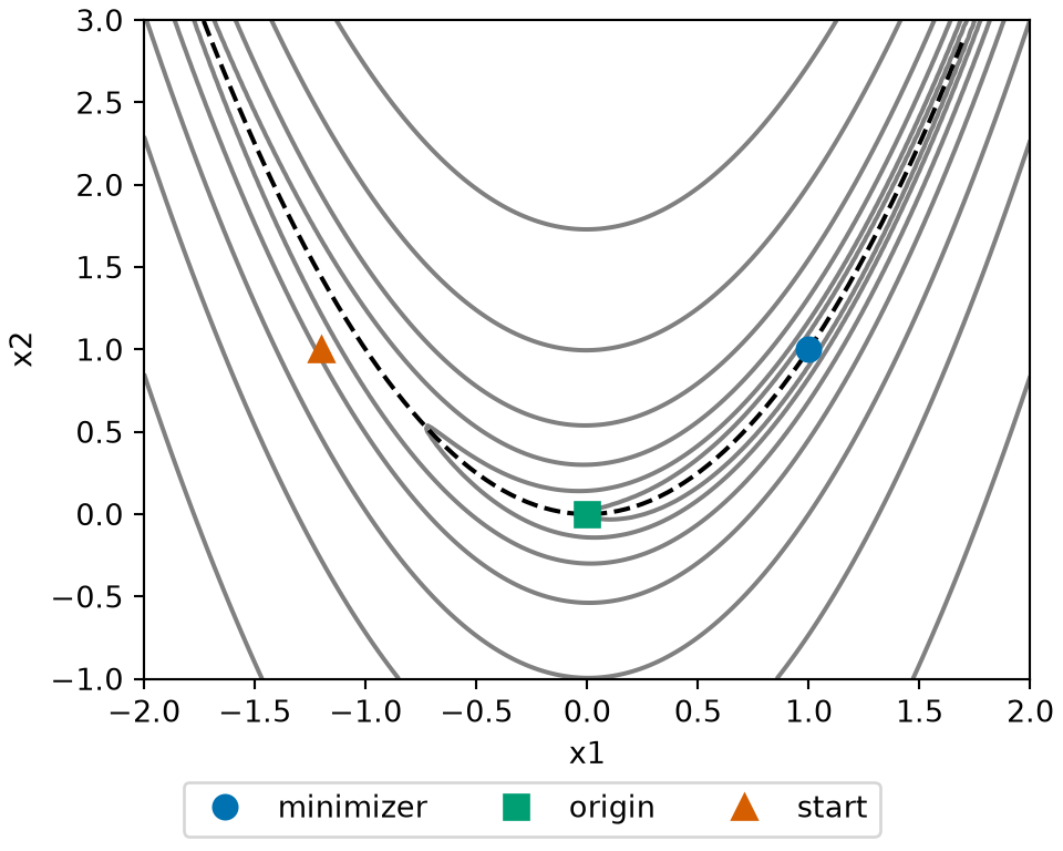
Example 9 (Values of the Rosenbrock function) We evaluate the Rosenbrock function at the minimizer \((1, 1)\), at the origin, and at the standard starting point \((-1.2, 1)\). Then we evaluate it along the curve \(x_2 = x_1^2\), which is the floor of a narrow, curved valley.
rosenbrock_rf <- function(x1, x2) 100 * (x2 - x1^2)^2 + (1 - x1)^2

points_rf <- list(minimizer = c(1, 1), origin = c(0, 0), start = c(-1.2, 1))
sapply(points_rf, function(p) round(rosenbrock_rf(p[1], p[2]), 3))
#> minimizer    origin     start
#>       0.0       1.0      24.2

# On the curve x2 = x1^2 the first term vanishes, leaving (1 - x1)^2.
x_curve_rf <- c(-1, 0, 0.5, 1, 2)
rbind(
  on_curve = rosenbrock_rf(x_curve_rf, x_curve_rf^2),
  formula = (1 - x_curve_rf)^2
)
#>          [,1] [,2] [,3] [,4] [,5]
#> on_curve    4    1 0.25    0    1
#> formula     4    1 0.25    0    1
import numpy as np
def rosenbrock_rf(x1, x2):
return 100 * (x2 - x1 ** 2) ** 2 + (1 - x1) ** 2
points_rf = {"minimizer": (1, 1), "origin": (0, 0), "start": (-1.2, 1)}
print({name: round(rosenbrock_rf(*p), 3) for name, p in points_rf.items()})
#> {'minimizer': 0, 'origin': 1, 'start': 24.2}
# On the curve x2 = x1^2 the first term vanishes, leaving (1 - x1)^2.
x_curve_rf = np.array([-1.0, 0.0, 0.5, 1.0, 2.0])
print("on_curve:", rosenbrock_rf(x_curve_rf, x_curve_rf ** 2))
#> on_curve: [4. 1. 0.25 0. 1. ]
print("formula: ", (1 - x_curve_rf) ** 2)
#> formula: [4. 1. 0.25 0. 1. ]The function is \(0\) at \((1, 1)\) and positive everywhere else, because both of its parts are non-negative and vanish together only when \(x_1 = 1\) and \(x_2 = 1\). So \((1, 1)\) is the global minimizer. At the starting point the value is 24.2, mostly from the first term, because \((-1.2, 1)\) is off the curve \(x_2 = x_1^2\). On the curve the function is \((1 - x_1)^2\), which varies slowly compared with the steep walls.
[Code]
library(ggplot2)
rf_grid <- expand.grid(
  x1 = seq(-2, 2, length.out = 201),
  x2 = seq(-1, 3, length.out = 201)
)
rf_grid$f <- rosenbrock_rf(rf_grid$x1, rf_grid$x2)
rf_points <- data.frame(
  name = names(points_rf),
  x1 = sapply(points_rf, `[`, 1),
  x2 = sapply(points_rf, `[`, 2)
)
rf_curve <- data.frame(x1 = seq(-2, 1.7, length.out = 200))
rf_curve$x2 <- rf_curve$x1^2
ggplot(rf_grid, aes(x1, x2)) +
  geom_contour(
    aes(z = f),
    colour = "grey60",
    breaks = c(1, 3, 10, 30, 100, 300, 1000)
  ) +
  geom_line(data = rf_curve, linetype = "dashed") +
  geom_point(aes(colour = name, shape = name), data = rf_points, size = 3) +
  scale_colour_manual(
    values = c(minimizer = "#0072B2", origin = "#009E73", start = "#D55E00")
  ) +
  scale_shape_manual(values = c(minimizer = 16, origin = 15, start = 17)) +
  coord_cartesian(xlim = c(-2, 2), ylim = c(-1, 3)) +
  labs(x = "x1", y = "x2", colour = NULL, shape = NULL) +
  theme(legend.position = "bottom")
[Code]
import matplotlib.pyplot as plt
import numpy as np

g1_rf, g2_rf = np.meshgrid(np.linspace(-2, 2, 201), np.linspace(-1, 3, 201))
fig, ax = plt.subplots(figsize=(5, 4), layout="constrained")
ax.contour(g1_rf, g2_rf, rosenbrock_rf(g1_rf, g2_rf), levels=[1, 3, 10, 30, 100, 300, 1000], colors="grey")
t_rf = np.linspace(-2, 1.7, 200)
ax.plot(t_rf, t_rf ** 2, color="black", linestyle="--")
style_rf = {"minimizer": ("#0072B2", "o"), "origin": ("#009E73", "s"), "start": ("#D55E00", "^")}
for name, p in points_rf.items():
    ax.plot(*p, color=style_rf[name][0], marker=style_rf[name][1], linestyle="", markersize=8, label=name)
ax.set_xlim(-2, 2)
#> (-2.0, 2.0)
ax.set_ylim(-1, 3)
#> (-1.0, 3.0)
ax.set_xlabel("x1")
ax.set_ylabel("x2")
fig.legend(loc="outside lower center", ncol=3)
plt.show()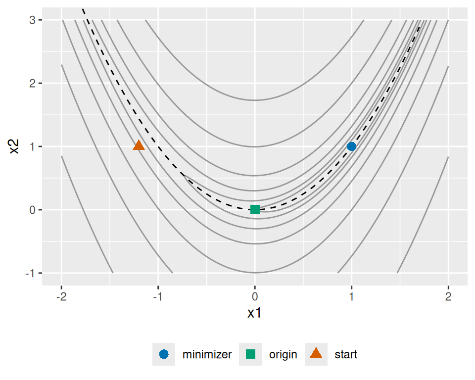
Definition 9 (Basin of attraction) For given step lengths, the basin of attraction of a local minimizer \(\mathord{\smash[b]{\underset{\raise.3ex\hbox{$\scriptstyle\sim$}}{x}}\vphantom{x}}^*\) under gradient descent is the set of starting points \({{\mathord{\smash[b]{\underset{\raise.3ex\hbox{$\scriptstyle\sim$}}{x}}\vphantom{x}}}^{(0)}}\) from which the iterates converge to \(\mathord{\smash[b]{\underset{\raise.3ex\hbox{$\scriptstyle\sim$}}{x}}\vphantom{x}}^*\) [4].
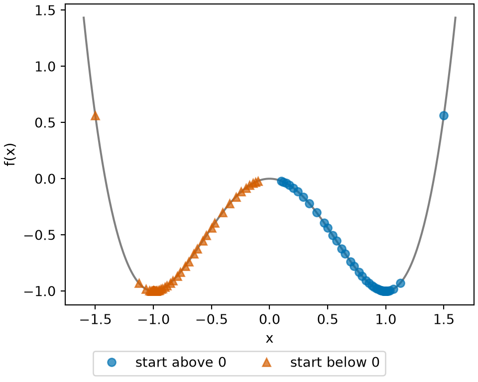
Example 10 (Basins of a double-well function) Let \(f(x) = x^4 - 2x^2\), so \(\frac{\partial}{\partial x} f(x) = 4x(x - 1)(x + 1)\) and the stationary points are \(-1\), \(0\) and \(1\). Both \(-1\) and \(1\) are local minimizers, with \(f(\pm 1) = -1\), and \(0\) is a local maximizer. We run gradient descent with the fixed step length \(s= 0.05\) for 200 steps from the starting points \(-1.5\), \(-0.5\), \(-0.1\), \(0.1\), \(0.5\), \(1.5\) and \(3\), and for three steps from \({{x}^{(0)}} = 4\).
basin_step_bs <- 0.05
basin_starts_bs <- c(-1.5, -0.5, -0.1, 0.1, 0.5, 1.5, 3)

# 200 steps from every starting point at once.
basin_final_bs <- basin_starts_bs
for (i in 1:200) {
  basin_slope_bs <- 4 * basin_final_bs^3 - 4 * basin_final_bs
  basin_final_bs <- basin_final_bs - basin_step_bs * basin_slope_bs
}
basin_end_bs <- signif(basin_final_bs, 3)
tibble::tibble(start = basin_starts_bs, end = basin_end_bs)
# The first step from 3.
basin_from_three_bs <- 3 - basin_step_bs * (4 * 3^3 - 4 * 3)

# Three steps from 4: the iterates grow in size.
basin_far_bs <- numeric(4)
basin_far_bs[1] <- 4
for (i in 1:3) {
  basin_slope_bs <- 4 * basin_far_bs[i]^3 - 4 * basin_far_bs[i]
  basin_far_bs[i + 1] <- basin_far_bs[i] - basin_step_bs * basin_slope_bs
}
signif(basin_far_bs, 3)
#> [1]       4.0      -8.0      92.8 -160000.0
basin_step_bs = 0.05
def basin_next_bs(x):
return x - basin_step_bs * (4 * x ** 3 - 4 * x)
def basin_gd_bs(x0, n_steps=200):
x = x0
for _ in range(n_steps):
x = basin_next_bs(x)
return x
basin_starts_bs = [-1.5, -0.5, -0.1, 0.1, 0.5, 1.5, 3]
for start in basin_starts_bs:
print(start, float(f"{basin_gd_bs(start):.3g}"))
#> -1.5 -1.0
#> -0.5 -1.0
#> -0.1 -1.0
#> 0.1 1.0
#> 0.5 1.0
#> 1.5 1.0
#> 3 -1.0
# Three steps from 4: the iterates grow in size.
basin_far_bs = [4.0]
for _ in range(3):
basin_far_bs.append(basin_next_bs(basin_far_bs[-1]))
print([float(f"{v:.3g}") for v in basin_far_bs])
#> [4.0, -8.0, 92.8, -160000.0]Each of the six starts between \(-1.5\) and \(1.5\) ends at \(-1\) or \(1\), whichever lies on its own side of \(0\), so for these starts the sign of the starting point decides which of the two the run reaches. A run from \(0\) itself never moves, because \(\frac{\partial}{\partial x} f(0) = 0\). The basin of attraction of \(1\) is not all of \((0, \infty)\): the first step from \({{x}^{(0)}} = 3\) lands at \(-1.8\), on the other side of \(0\), and the run ends at \(-1\). From \({{x}^{(0)}} = 4\) the iterates, starting with \({{x}^{(0)}}\) itself, are \(4\), \(-8\), \(92.8\) and \(-1.6\times 10^{5}\), which grow in absolute value at every step shown. Both of these starts are far from \(0\), where the derivative is large and so the step \(s\frac{\partial}{\partial x} f(x)\) is long. From \({{x}^{(0)}} = 3\) that step is \(96\,s\) long, so the first step stays on the positive side of \(0\) only when \(s\) is below \(0.03125\). So the basin of \(1\) depends on \(s\), and with \(s= 0.05\) the basin is not a half-line.
[Code]
# Uses basin_step_bs and basin_starts_bs from the example above.
basin_runs_bf <- matrix(0, nrow = 31, ncol = 6)
basin_runs_bf[1, ] <- basin_starts_bs[1:6]
for (i in 1:30) {
  basin_prev_bf <- basin_runs_bf[i, ]
  basin_slope_bf <- 4 * basin_prev_bf^3 - 4 * basin_prev_bf
  basin_runs_bf[i + 1, ] <- basin_prev_bf - basin_step_bs * basin_slope_bf
}
basin_side_bf <- ifelse(
  basin_starts_bs[1:6] > 0, "start above 0", "start below 0"
)
basin_x_bf <- as.vector(basin_runs_bf)
basin_side_all_bf <- rep(basin_side_bf, each = 31)
basin_paths_bf <- tibble::tibble(x = basin_x_bf, side = basin_side_all_bf)
basin_paths_bf$cost <- basin_paths_bf$x^4 - 2 * basin_paths_bf$x^2
basin_grid_bf <- seq(-1.6, 1.6, length.out = 321)
basin_curve_bf <- tibble::tibble(
  x = basin_grid_bf, cost = basin_grid_bf^4 - 2 * basin_grid_bf^2
)
basin_colours_bf <- c("start above 0" = "#0072B2", "start below 0" = "#D55E00")
ggplot2::ggplot(basin_curve_bf, ggplot2::aes(x, cost)) +
  ggplot2::geom_line(colour = "grey60") +
  ggplot2::geom_point(
    data = basin_paths_bf,
    ggplot2::aes(colour = side, shape = side), alpha = 0.7
  ) +
  ggplot2::scale_colour_manual(values = basin_colours_bf) +
  ggplot2::labs(x = "x", y = "f(x)", colour = NULL, shape = NULL) +
  ggplot2::theme(legend.position = "bottom")
[Code]
import matplotlib.pyplot as plt
import numpy as np

def basin_cost_bf(x):
    return x ** 4 - 2 * x ** 2

fig, ax = plt.subplots(figsize=(5, 4), layout="constrained")
grid_bf = np.linspace(-1.6, 1.6, 321)
ax.plot(grid_bf, basin_cost_bf(grid_bf), color="grey")
#> [<matplotlib.lines.Line2D object at 0x7f7fe9028050>]
for start in sorted(basin_starts_bs[:6], reverse=True):
    x = [start]
    for _ in range(30):
        x.append(basin_next_bs(x[-1]))
    x = np.array(x)
    above = start > 0
    ax.plot(x, basin_cost_bf(x), linestyle="", alpha=0.7,
            color="#0072B2" if above else "#D55E00",
            marker="o" if above else "^",
            label=("start above 0" if above else "start below 0")
            if abs(start) == 0.1 else None)
#> [<matplotlib.lines.Line2D object at 0x7f7fe9028190>]
#> [<matplotlib.lines.Line2D object at 0x7f7fe90282d0>]
#> [<matplotlib.lines.Line2D object at 0x7f7fe9028410>]
#> [<matplotlib.lines.Line2D object at 0x7f7fe9028550>]
#> [<matplotlib.lines.Line2D object at 0x7f7fe9028690>]
#> [<matplotlib.lines.Line2D object at 0x7f7fe90287d0>]
ax.set_xlabel("x")
#> Text(0.5, 0, 'x')
ax.set_ylabel("f(x)")
#> Text(0, 0.5, 'f(x)')
fig.legend(loc="outside lower center", ncol=2)
#> <matplotlib.legend.Legend object at 0x7f7fe9028910>
plt.show()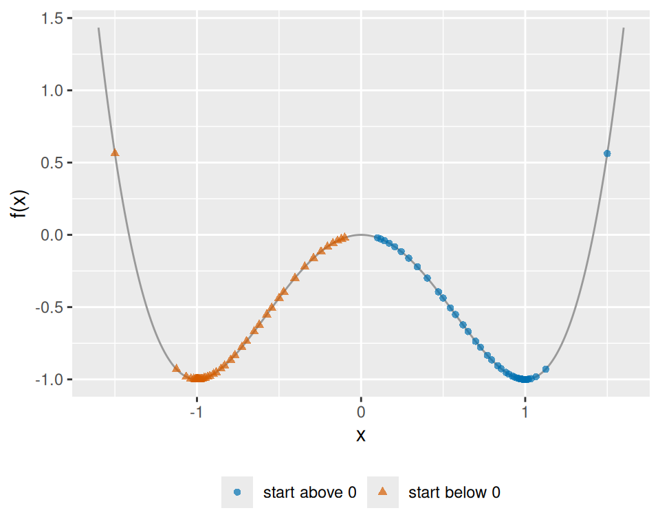
Proposition 1 (Divergence of gradient descent on the double-well function) Let \(f(x) = x^4 - 2x^2\), and run gradient descent with a fixed step length \(s> 0\). If \({{x}^{(0)}}\) satisfies
\[ {{x}^{(0)}}^2 > 1 + \frac{1}{2s}, \]
then \(\mathopen{}\left|{{x}^{(t)}}\right|\mathclose{} \to \infty\) as \(t \to \infty\).
Proof. The derivative is \(\frac{\partial}{\partial x} f(x) = 4x^3 - 4x\), so one step of gradient descent gives
\[ \begin{aligned} {{x}^{(t+1)}} &= {{x}^{(t)}} - s\,\mathopen{}\left(4 {{x}^{(t)}}^3 - 4 {{x}^{(t)}}\right)\mathclose{} && \text{(gradient descent step)} \\ &= -{{x}^{(t)}}\,\mathopen{}\left(4s{{x}^{(t)}}^2 - 4s- 1\right)\mathclose{}. && \text{(factor out } -{{x}^{(t)}} \text{)} \end{aligned} \]
Write \(m(x) \stackrel{\text{def}}{=}4sx^2 - 4s- 1\). Then \(\mathopen{}\left|{{x}^{(t+1)}}\right|\mathclose{} = \mathopen{}\left|{{x}^{(t)}}\right|\mathclose{}\, m({{x}^{(t)}})\) whenever \(m({{x}^{(t)}}) \ge 0\). Now \(m(x) > 1\) exactly when \(x^2 > 1 + 1 / (2s)\), and \(m(x)\) increases with \(x^2\). So if \({{x}^{(t)}}\) satisfies the condition, then \(\mathopen{}\left|{{x}^{(t+1)}}\right|\mathclose{} > \mathopen{}\left|{{x}^{(t)}}\right|\mathclose{}\), and \({{x}^{(t+1)}}\) satisfies it too. By induction on \(t\), every iterate satisfies it. Since \(\mathopen{}\left|{{x}^{(t)}}\right|\mathclose{}\) increases at every step, \({{x}^{(t)}}^2 \ge {{x}^{(0)}}^2\), and so \(m({{x}^{(t)}}) \ge m({{x}^{(0)}}) > 1\). Hence \(\mathopen{}\left|{{x}^{(t)}}\right|\mathclose{} \ge m({{x}^{(0)}})^t \mathopen{}\left|{{x}^{(0)}}\right|\mathclose{}\), which tends to \(\infty\).
Corollary 1 (Basins of the double-well function are bounded) Let \(f(x) = x^4 - 2x^2\), and run gradient descent with a fixed step length \(s> 0\). Every start \({{x}^{(0)}}\) in the basin of attraction of a local minimizer of \(f\) satisfies
\[ {{x}^{(0)}}^2 \le 1 + \frac{1}{2s}. \]
Proof. The iterates from a start in the basin converge to a local minimizer, so they do not diverge to \(\infty\). By Proposition 1, the start therefore does not satisfy \({{x}^{(0)}}^2 > 1 + 1 / (2s)\).
Example 11 (Divergent starts on the double-well function for three step lengths) For \(f(x) = x^4 - 2x^2\), Proposition 1 says that gradient descent diverges to \(\infty\) from every start with \(\mathopen{}\left|{{x}^{(0)}}\right|\mathclose{}\) above \(\sqrt{1 + 1 / (2s)}\). This bound is \(7.14\) for \(s= 0.01\), \(3.32\) for \(s= 0.05\), and \(2.45\) for \(s= 0.1\). The derivative \(4x^3 - 4x\) is unbounded, as is the second derivative \(12x^2 - 4\), so the step \(s\frac{\partial}{\partial x} f(x)\) grows without bound with \(x\), and a far start overshoots. By Proposition 1, every fixed step length fails to converge from some starts. A larger step length lowers the bound, so more starts are guaranteed to diverge. By Corollary 1, each basin of attraction lies within the same bounded interval, which narrows as \(s\) grows. In the earlier basin example, \(s= 0.05\), and the start \(4\) lies above the bound \(3.32\), which is why its iterates grow.
Definition 10 (Plateau) Let \(f : \mathbb{R}^p \to \mathbb{R}\) be a function with a gradient at every point of a region, and let \(\epsilon > 0\) be a tolerance. The region is a plateau of \(f\) if the Euclidean norm of the gradient satisfies
\[ 0 < \mathopen{}\left\lVert\frac{\partial}{\partial \mathord{\smash[b]{\underset{\raise.3ex\hbox{$\scriptstyle\sim$}}{x}}\vphantom{x}}} f(\mathord{\smash[b]{\underset{\raise.3ex\hbox{$\scriptstyle\sim$}}{x}}\vphantom{x}})\right\rVert\mathclose{} < \epsilon \]
at every point \(\mathord{\smash[b]{\underset{\raise.3ex\hbox{$\scriptstyle\sim$}}{x}}\vphantom{x}}\) of the region. The function is then nearly flat on the region, and the region contains no stationary point.
Example 12 (A cost with no stationary point)
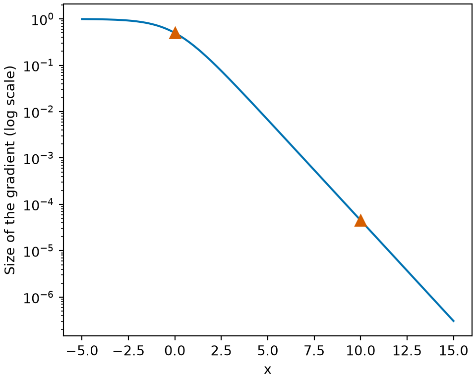
Let \(f(x) = \log\mathopen{}\left(1 + \text{e}^{-x}\right)\mathclose{}\). Its derivative is \(\frac{\partial}{\partial x} f(x) = -1 / (1 + \text{e}^{x})\), which is negative for every \(x\), so \(f\) has no stationary point at all.
At \(x = 0\) the gradient has size \(0.5\). At \(x = 10\) it has size \(4.54\times 10^{-5}\), which is small but not zero. A step of gradient descent subtracts the gradient times the step length. The gradient is negative, so the iterates keep moving to the right, more and more slowly. With tolerance \(\epsilon = 10^{-4}\), the region \(x \ge 10\) is a plateau (Definition 10). A run that enters this plateau has not converged; the run has only slowed down.
[Code]
plateau_grid_pf <- seq(-5, 15, length.out = 401)
plateau_exp_pf <- exp(plateau_grid_pf)
plateau_size_pf <- 1 / (1 + plateau_exp_pf)
plateau_curve_pf <- tibble::tibble(x = plateau_grid_pf, size = plateau_size_pf)
plateau_marks_x_pf <- c(0, 10)
plateau_marks_exp_pf <- exp(plateau_marks_x_pf)
plateau_marks_size_pf <- 1 / (1 + plateau_marks_exp_pf)
plateau_marks_pf <- tibble::tibble(
  x = plateau_marks_x_pf, size = plateau_marks_size_pf
)
plateau_aes_pf <- ggplot2::aes(x, size)
ggplot2::ggplot(plateau_curve_pf, plateau_aes_pf) +
  ggplot2::geom_line(colour = "#0072B2") +
  ggplot2::geom_point(
    data = plateau_marks_pf, colour = "#D55E00", shape = 17, size = 3
  ) +
  ggplot2::scale_y_log10() +
  ggplot2::labs(x = "x", y = "Size of the gradient (log scale)")
[Code]
import matplotlib.pyplot as plt
import numpy as np

plateau_grid_pf = np.linspace(-5, 15, 401)
plateau_marks_pf = np.array([0, 10])
fig, ax = plt.subplots(figsize=(5, 4), layout="constrained")
ax.plot(plateau_grid_pf, 1 / (1 + np.exp(plateau_grid_pf)), color="#0072B2")
#> [<matplotlib.lines.Line2D object at 0x7f7fe8c3d090>]
ax.plot(plateau_marks_pf, 1 / (1 + np.exp(plateau_marks_pf)),
        color="#D55E00", marker="^", markersize=8, linestyle="")
#> [<matplotlib.lines.Line2D object at 0x7f7fe8c3d1d0>]
ax.set_yscale("log")
ax.set_xlabel("x")
#> Text(0.5, 0, 'x')
ax.set_ylabel("Size of the gradient (log scale)")
#> Text(0, 0.5, 'Size of the gradient (log scale)')
plt.show()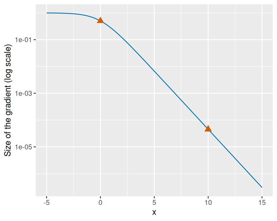
Definition 11 (Armijo condition) Let \(f : \mathbb{R}^p \to \mathbb{R}\) have first partial derivatives, let \(\mathord{\smash[b]{\underset{\raise.3ex\hbox{$\scriptstyle\sim$}}{x}}\vphantom{x}}\in \mathbb{R}^p\), and let \(\mathord{\smash[b]{\underset{\raise.3ex\hbox{$\scriptstyle\sim$}}{g}}\vphantom{g}} \stackrel{\text{def}}{=}\frac{\partial}{\partial \mathord{\smash[b]{\underset{\raise.3ex\hbox{$\scriptstyle\sim$}}{x}}\vphantom{x}}} f(\mathord{\smash[b]{\underset{\raise.3ex\hbox{$\scriptstyle\sim$}}{x}}\vphantom{x}})\). A step length \(s > 0\) satisfies the Armijo condition [5] with constant \(c \in (0, 1)\) at \(\mathord{\smash[b]{\underset{\raise.3ex\hbox{$\scriptstyle\sim$}}{x}}\vphantom{x}}\) if
\[ f(\mathord{\smash[b]{\underset{\raise.3ex\hbox{$\scriptstyle\sim$}}{x}}\vphantom{x}}- s \mathord{\smash[b]{\underset{\raise.3ex\hbox{$\scriptstyle\sim$}}{g}}\vphantom{g}}) \le f(\mathord{\smash[b]{\underset{\raise.3ex\hbox{$\scriptstyle\sim$}}{x}}\vphantom{x}}) - c\, s\, \mathopen{}\left\lVert\mathord{\smash[b]{\underset{\raise.3ex\hbox{$\scriptstyle\sim$}}{g}}\vphantom{g}}\right\rVert\mathclose{}^2. \]
Example 13 (The Armijo condition on a parabola) Let \(f(x) = x^2\) and \(x = 2\), so \(g = f'(2) = 4\) and \(\mathopen{}\left\lVert g\right\rVert\mathclose{}^2 = 16\). With \(c = 1/4\), the condition on a step length \(s > 0\) is
\[ \begin{aligned} (2 - 4s)^2 &\le 4 - 4s && \text{(} f(2 - 4s) \le f(2) - c\, s\, \mathopen{}\left\lVert g\right\rVert\mathclose{}^2 \text{)} \\ 4 - 16 s + 16 s^2 &\le 4 - 4s && \text{(expand the square)} \\ 16 s^2 &\le 12 s && \text{(add } 16 s - 4 \text{ to both sides)} \\ s &\le 3/4. && \text{(divide by } 16 s > 0 \text{)} \end{aligned} \]
So \(s = 1/2\) satisfies the condition: \(f(0) = 0 \le 4 - 2 = 2\). And \(s = 1\) does not: \(f(-2) = 4 > 4 - 4 = 0\).
Definition 12 (Backtracking line search) Let \(s_0 > 0\) be an initial step length, \(\beta \in (0, 1)\) a shrink factor, and \(c \in (0, 1)\). Backtracking line search [5] is the line search that chooses \(s^{(t)}\) to be the largest of \(s_0, \beta s_0, \beta^2 s_0, \ldots\) that satisfies the Armijo condition with constant \(c\) at \(\mathord{\smash[b]{\underset{\raise.3ex\hbox{$\scriptstyle\sim$}}{x}}\vphantom{x}}^{(t)}\).
Example 14 (Backtracking on a parabola) For \(f(x) = x^2\) at \(x = 2\) with \(c = 1/4\), the Armijo condition holds exactly when \(s \le 3/4\) (Example 13). With \(s_0 = 1\) and \(\beta = 1/2\), the trial step lengths are \(1, 1/2, 1/4, \ldots\). The first, \(s = 1\), exceeds \(3/4\) and is rejected. The second, \(s = 1/2\), is at most \(3/4\) and is accepted. So backtracking chooses \(s^{(0)} = 1/2\), after two evaluations of \(f\).
Theorem 2 (A bound on the error of gradient descent on a quadratic) Let \(\mathbf{S}\) be a \(p \times p\) positive definite matrix with eigenvalues \(\lambda_1, \ldots, \lambda_p\), let \(\mathord{\smash[b]{\underset{\raise.3ex\hbox{$\scriptstyle\sim$}}{c}}\vphantom{c}} \in \mathbb{R}^p\), and let \(f(\mathord{\smash[b]{\underset{\raise.3ex\hbox{$\scriptstyle\sim$}}{x}}\vphantom{x}}) = \tfrac{1}{2}\,{\mathord{\smash[b]{\underset{\raise.3ex\hbox{$\scriptstyle\sim$}}{x}}\vphantom{x}}}^{\top} \mathbf{S} \mathord{\smash[b]{\underset{\raise.3ex\hbox{$\scriptstyle\sim$}}{x}}\vphantom{x}} - \mathord{\smash[b]{\underset{\raise.3ex\hbox{$\scriptstyle\sim$}}{c}}\vphantom{c}} \cdot \mathord{\smash[b]{\underset{\raise.3ex\hbox{$\scriptstyle\sim$}}{x}}\vphantom{x}}\), whose unique minimizer is \(\mathord{\smash[b]{\underset{\raise.3ex\hbox{$\scriptstyle\sim$}}{x}}\vphantom{x}}^* = \mathbf{S}^{-1} \mathord{\smash[b]{\underset{\raise.3ex\hbox{$\scriptstyle\sim$}}{c}}\vphantom{c}}\) (Theorem 2 in Newton’s Method). Gradient descent with a fixed step length \(s> 0\) from any \({{\mathord{\smash[b]{\underset{\raise.3ex\hbox{$\scriptstyle\sim$}}{x}}\vphantom{x}}}^{(0)}}\) has errors satisfying, for \(t = 1, 2, \ldots\),
\[ \mathopen{}\left\lVert{{\mathord{\smash[b]{\underset{\raise.3ex\hbox{$\scriptstyle\sim$}}{x}}\vphantom{x}}}^{(t)}} - \mathord{\smash[b]{\underset{\raise.3ex\hbox{$\scriptstyle\sim$}}{x}}\vphantom{x}}^*\right\rVert\mathclose{} \le \rho(s)^t\,\mathopen{}\left\lVert{{\mathord{\smash[b]{\underset{\raise.3ex\hbox{$\scriptstyle\sim$}}{x}}\vphantom{x}}}^{(0)}} - \mathord{\smash[b]{\underset{\raise.3ex\hbox{$\scriptstyle\sim$}}{x}}\vphantom{x}}^*\right\rVert\mathclose{}, \qquad \rho(s) \stackrel{\text{def}}{=}\max_{1 \le i \le p} \mathopen{}\left|1 - s\,\lambda_i\right|\mathclose{}. \]
Proof. Let \(\mathord{\smash[b]{\underset{\raise.3ex\hbox{$\scriptstyle\sim$}}{e}}\vphantom{e}}^{(t)} \stackrel{\text{def}}{=}{{\mathord{\smash[b]{\underset{\raise.3ex\hbox{$\scriptstyle\sim$}}{x}}\vphantom{x}}}^{(t)}} - \mathord{\smash[b]{\underset{\raise.3ex\hbox{$\scriptstyle\sim$}}{x}}\vphantom{x}}^*\) be the error at step \(t\). The gradient of \(f\) is \(\frac{\partial}{\partial \mathord{\smash[b]{\underset{\raise.3ex\hbox{$\scriptstyle\sim$}}{x}}\vphantom{x}}} f(\mathord{\smash[b]{\underset{\raise.3ex\hbox{$\scriptstyle\sim$}}{x}}\vphantom{x}}) = \mathbf{S}\mathord{\smash[b]{\underset{\raise.3ex\hbox{$\scriptstyle\sim$}}{x}}\vphantom{x}}- \mathord{\smash[b]{\underset{\raise.3ex\hbox{$\scriptstyle\sim$}}{c}}\vphantom{c}}\) (see the proof of Theorem 2 in Newton’s Method), and \(\mathord{\smash[b]{\underset{\raise.3ex\hbox{$\scriptstyle\sim$}}{c}}\vphantom{c}} = \mathbf{S}\mathord{\smash[b]{\underset{\raise.3ex\hbox{$\scriptstyle\sim$}}{x}}\vphantom{x}}^*\), so
\[ \begin{aligned} \mathord{\smash[b]{\underset{\raise.3ex\hbox{$\scriptstyle\sim$}}{e}}\vphantom{e}}^{(t+1)} &= {{\mathord{\smash[b]{\underset{\raise.3ex\hbox{$\scriptstyle\sim$}}{x}}\vphantom{x}}}^{(t)}} - s\,(\mathbf{S}{{\mathord{\smash[b]{\underset{\raise.3ex\hbox{$\scriptstyle\sim$}}{x}}\vphantom{x}}}^{(t)}} - \mathord{\smash[b]{\underset{\raise.3ex\hbox{$\scriptstyle\sim$}}{c}}\vphantom{c}}) - \mathord{\smash[b]{\underset{\raise.3ex\hbox{$\scriptstyle\sim$}}{x}}\vphantom{x}}^* && \text{(definition of gradient descent)} \\ &= {{\mathord{\smash[b]{\underset{\raise.3ex\hbox{$\scriptstyle\sim$}}{x}}\vphantom{x}}}^{(t)}} - s\,\mathbf{S}({{\mathord{\smash[b]{\underset{\raise.3ex\hbox{$\scriptstyle\sim$}}{x}}\vphantom{x}}}^{(t)}} - \mathord{\smash[b]{\underset{\raise.3ex\hbox{$\scriptstyle\sim$}}{x}}\vphantom{x}}^*) - \mathord{\smash[b]{\underset{\raise.3ex\hbox{$\scriptstyle\sim$}}{x}}\vphantom{x}}^* && \text{(} \mathord{\smash[b]{\underset{\raise.3ex\hbox{$\scriptstyle\sim$}}{c}}\vphantom{c}} = \mathbf{S}\mathord{\smash[b]{\underset{\raise.3ex\hbox{$\scriptstyle\sim$}}{x}}\vphantom{x}}^* \text{)} \\ &= (\mathbf{I}_p - s\,\mathbf{S})\,\mathord{\smash[b]{\underset{\raise.3ex\hbox{$\scriptstyle\sim$}}{e}}\vphantom{e}}^{(t)}. && \text{(collect the terms in } \mathord{\smash[b]{\underset{\raise.3ex\hbox{$\scriptstyle\sim$}}{e}}\vphantom{e}}^{(t)} \text{)} \end{aligned} \]
By induction on \(t\), \(\mathord{\smash[b]{\underset{\raise.3ex\hbox{$\scriptstyle\sim$}}{e}}\vphantom{e}}^{(t)} = (\mathbf{I}_p - s\,\mathbf{S})^t\,\mathord{\smash[b]{\underset{\raise.3ex\hbox{$\scriptstyle\sim$}}{e}}\vphantom{e}}^{(0)}\). Write \(\mathbf{S} = \mathbf{Q}\mathbf{\Lambda}{\mathbf{Q}}^{\top}\) (spectral theorem). Then \(\mathbf{I}_p - s\,\mathbf{S} = \mathbf{Q}(\mathbf{I}_p - s\,\mathbf{\Lambda}){\mathbf{Q}}^{\top}\) because \(\mathbf{Q}{\mathbf{Q}}^{\top} = \mathbf{I}_p\), and the \(t\)th power cancels each inner \({\mathbf{Q}}^{\top}\mathbf{Q} = \mathbf{I}_p\), so
\[ \begin{aligned} \mathopen{}\left\lVert\mathord{\smash[b]{\underset{\raise.3ex\hbox{$\scriptstyle\sim$}}{e}}\vphantom{e}}^{(t)}\right\rVert\mathclose{} &= \mathopen{}\left\lVert\mathbf{Q}(\mathbf{I}_p - s\,\mathbf{\Lambda})^t{\mathbf{Q}}^{\top}\mathord{\smash[b]{\underset{\raise.3ex\hbox{$\scriptstyle\sim$}}{e}}\vphantom{e}}^{(0)}\right\rVert\mathclose{} && \text{(the factorization above)} \\ &= \mathopen{}\left\lVert(\mathbf{I}_p - s\,\mathbf{\Lambda})^t{\mathbf{Q}}^{\top}\mathord{\smash[b]{\underset{\raise.3ex\hbox{$\scriptstyle\sim$}}{e}}\vphantom{e}}^{(0)}\right\rVert\mathclose{} && \text{(orthogonal matrices preserve length)} \\ &\le \rho(s)^t\,\mathopen{}\left\lVert{\mathbf{Q}}^{\top}\mathord{\smash[b]{\underset{\raise.3ex\hbox{$\scriptstyle\sim$}}{e}}\vphantom{e}}^{(0)}\right\rVert\mathclose{} && \text{(each coordinate is multiplied by } (1 - s\lambda_i)^t \text{)} \\ &= \rho(s)^t\,\mathopen{}\left\lVert\mathord{\smash[b]{\underset{\raise.3ex\hbox{$\scriptstyle\sim$}}{e}}\vphantom{e}}^{(0)}\right\rVert\mathclose{}. && \text{(orthogonal matrices preserve length)} \end{aligned} \]
The length-preserving steps apply orthogonal matrices preserve length. The inequality holds because \(\mathbf{I}_p - s\,\mathbf{\Lambda}\) is diagonal, so its \(t\)th power multiplies coordinate \(i\) by \((1 - s\,\lambda_i)^t\), whose absolute value is at most \(\rho(s)^t\).
Example 15 (The error multiplier for a step length of one quarter) Let \(\mathbf{S} = \begin{bmatrix} 2 & 1 \\ 1 & 2 \end{bmatrix}\) with eigenvalues \(3\) and \(1\) (eigenvalue example), and \(\mathord{\smash[b]{\underset{\raise.3ex\hbox{$\scriptstyle\sim$}}{c}}\vphantom{c}} = \mathord{\smash[b]{\underset{\raise.3ex\hbox{$\scriptstyle\sim$}}{0}}\vphantom{0}}_{2 \times 1}\), so \(\mathord{\smash[b]{\underset{\raise.3ex\hbox{$\scriptstyle\sim$}}{x}}\vphantom{x}}^* = \mathord{\smash[b]{\underset{\raise.3ex\hbox{$\scriptstyle\sim$}}{0}}\vphantom{0}}_{2 \times 1}\). With \(s= 0.25\), the factors \(1 - s\,\lambda_i\) are \(0.25\) and \(0.75\), so \(\rho(s) = 0.75\) and
\[ \mathopen{}\left\lVert{{\mathord{\smash[b]{\underset{\raise.3ex\hbox{$\scriptstyle\sim$}}{x}}\vphantom{x}}}^{(t)}}\right\rVert\mathclose{} \le 0.75^t\,\mathopen{}\left\lVert{{\mathord{\smash[b]{\underset{\raise.3ex\hbox{$\scriptstyle\sim$}}{x}}\vphantom{x}}}^{(0)}}\right\rVert\mathclose{}. \]
Along the eigenvector for \(\lambda= 3\) the error shrinks fast, and along the eigenvector for \(\lambda= 1\) it shrinks slowly; the bound follows the slower one.
Theorem 3 (The best constant step length) In the setting of Theorem 2, let \(\lambda_{\min}\) and \(\lambda_{\max}\) be the smallest and largest eigenvalues of \(\mathbf{S}\). The factor \(\rho(s) = \max_i \mathopen{}\left|1 - s\,\lambda_i\right|\mathclose{}\) of Theorem 2 is smallest over \(s> 0\) at
\[ s^* = \frac{2}{\lambda_{\min} + \lambda_{\max}}, \]
where
\[ \rho(s^*) = \frac{\kappa- 1}{\kappa+ 1}, \qquad \kappa= \kappa(\mathbf{S}), \]
the condition number of \(\mathbf{S}\).
Proof. For \(s> 0\), each \(1 - s\,\lambda_i\) lies between \(u_{\min} \stackrel{\text{def}}{=}1 - s\,\lambda_{\max}\) and \(u_{\max} \stackrel{\text{def}}{=}1 - s\,\lambda_{\min}\), so \(\mathopen{}\left|1 - s\,\lambda_i\right|\mathclose{} \le {\max\mathopen{}\left(u_{\max}, -u_{\min}\right)\mathclose{}}\). Both \(\lambda_{\min}\) and \(\lambda_{\max}\) occur among the \(\lambda_i\), and \(\mathopen{}\left|u_{\max}\right|\mathclose{} \ge u_{\max}\) and \(\mathopen{}\left|u_{\min}\right|\mathclose{} \ge -u_{\min}\), so the maximum is attained:
\[ \rho(s) = {\max\mathopen{}\left(1 - s\,\lambda_{\min},\ s\,\lambda_{\max} - 1\right)\mathclose{}}. \]
The first expression is strictly decreasing in \(s\), and the second is strictly increasing, and they coincide when
\[ \begin{aligned} 1 - s\,\lambda_{\min} &= s\,\lambda_{\max} - 1 && \text{(set the two expressions equal)} \\ 2 &= s\,(\lambda_{\min} + \lambda_{\max}) && \text{(collect the terms in } s\text{)} \\ s&= \frac{2}{\lambda_{\min} + \lambda_{\max}} = s^*. && \text{(divide)} \end{aligned} \]
For \(s< s^*\), \(\rho(s)\) is at least the decreasing expression, which exceeds its value at \(s^*\). For \(s> s^*\), \(\rho(s)\) is at least the increasing expression, which exceeds its value at \(s^*\). So \(s^*\) is the minimizer, and
\[ \begin{aligned} \rho(s^*) &= 1 - \frac{2\,\lambda_{\min}}{\lambda_{\min} + \lambda_{\max}} && \text{(first expression at } s^* \text{)} \\ &= \frac{\lambda_{\max} - \lambda_{\min}}{\lambda_{\max} + \lambda_{\min}} && \text{(common denominator)} \\ &= \frac{\kappa- 1}{\kappa+ 1}. && \text{(divide the numerator and denominator by } \lambda_{\min} \text{)} \end{aligned} \]
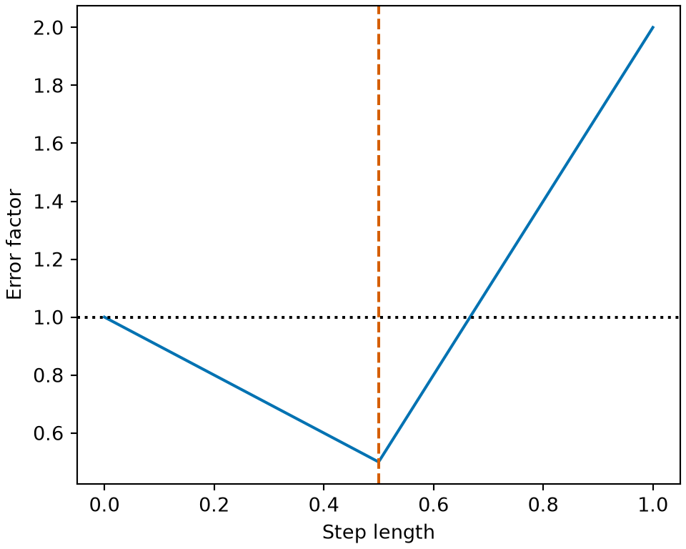
Example 16 (The best step length for eigenvalues 3 and 1) For \(\mathbf{S} = \begin{bmatrix} 2 & 1 \\ 1 & 2 \end{bmatrix}\) with eigenvalues \(3\) and \(1\), Theorem 3 gives \(s^* = 2 / (3 + 1) = 0.5\), \(\kappa= 3\) (condition number example), and \(\rho(s^*) = (3 - 1) / (3 + 1) = 0.5\). A grid search over \(s= 0.01, 0.02, \ldots, 1\) finds the smallest \(\rho(s)\) at \(s= 0.5\), the same step length. Each step then multiplies the error by at most \(0.5\).
[Code]
bcs_grid_pf <- seq(0, 1, length.out = 401)
bcs_first_pf <- abs(1 - 3 * bcs_grid_pf)
bcs_second_pf <- abs(1 - bcs_grid_pf)
bcs_rho_pf <- pmax(bcs_first_pf, bcs_second_pf)
bcs_curve_pf <- tibble::tibble(s = bcs_grid_pf, rho = bcs_rho_pf)
bcs_aes_pf <- ggplot2::aes(s, rho)
ggplot2::ggplot(bcs_curve_pf, bcs_aes_pf) +
  ggplot2::geom_line(colour = "#0072B2") +
  ggplot2::geom_hline(yintercept = 1, linetype = "dotted") +
  ggplot2::geom_vline(
    xintercept = 0.5, colour = "#D55E00", linetype = "dashed"
  ) +
  ggplot2::labs(x = "Step length", y = "Error factor")
[Code]
import matplotlib.pyplot as plt
import numpy as np

bcs_grid_pf = np.linspace(0, 1, 401)
bcs_rho_pf = np.maximum(np.abs(1 - 3 * bcs_grid_pf), np.abs(1 - bcs_grid_pf))
fig, ax = plt.subplots(figsize=(5, 4), layout="constrained")
ax.plot(bcs_grid_pf, bcs_rho_pf, color="#0072B2")
#> [<matplotlib.lines.Line2D object at 0x7f7fe8ab9310>]
ax.axhline(1, color="black", linestyle=":")
#> <matplotlib.lines.Line2D object at 0x7f7fe8ab9450>
ax.axvline(0.5, color="#D55E00", linestyle="--")
#> <matplotlib.lines.Line2D object at 0x7f7fe8ab9590>
ax.set_xlabel("Step length")
#> Text(0.5, 0, 'Step length')
ax.set_ylabel("Error factor")
#> Text(0, 0.5, 'Error factor')
plt.show()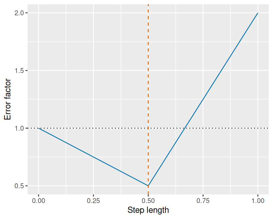
Exercise 1 (Which step lengths shrink the error bound) In the setting of Theorem 2, find all \(s> 0\) with \(\rho(s) < 1\), and write the answer as a condition on \(s\) that involves \(\lambda_{\max}\).
Solution 1. \(\rho(s) < 1\) says that \(\mathopen{}\left|1 - s\,\lambda_i\right|\mathclose{} < 1\) for every \(i\), which is \(-1 < 1 - s\,\lambda_i < 1\). The right inequality holds for every \(s> 0\) because \(\lambda_i > 0\). The left inequality is \(s\,\lambda_i < 2\), that is, \(s< 2 / \lambda_i\). These \(p\) inequalities, one for each eigenvalue, all hold exactly when the inequality for the largest eigenvalue holds, since it is the most restrictive:
\[ 0 < s< \frac{2}{\lambda_{\max}}. \]
Exercise 2 (The best step length for eigenvalues 1 and 9) In gradient descent, a fixed step length that is too short converges slowly, and one that is too long diverges. Theorem 3 gives the best one from the eigenvalues of \(\mathbf{S}\).
Let \(\mathbf{S} = \begin{bmatrix} 1 & 0 \\ 0 & 9 \end{bmatrix}\). Using Theorem 3, find \(s^*\).
Solution 2. \(\mathbf{S}\) is diagonal, so its eigenvalues are its diagonal entries \(1\) and \(9\). Then
\[ s^* = \frac{2}{1 + 9} = 0.2. \]
Exercise 3 (The best error factor for eigenvalues 1 and 9) In the setting of Exercise 2, find \(\rho(s^*)\).
Solution 3. The condition number is \(\kappa(\mathbf{S}) = 9 / 1 = 9\), so by Theorem 3
\[ \rho(s^*) = \frac{9 - 1}{9 + 1} = 0.8. \]
Exercise 4 (Steps to cut the error bound by a factor of ten) In the setting of Exercise 2 and Exercise 3, find the smallest \(t = 1, 2, \ldots\) with \(\rho(s^*)^t \le 0.1\).
Solution 4. From Solution 3, \(\rho(s^*) = 0.8\). Taking logarithms, \(\rho(s^*)^t \le 0.1\) becomes \(t \ln \rho(s^*) \le \ln 0.1\). Here \(\ln \rho(s^*) < 0\), so dividing by it flips the inequality: \(t \ge \ln 0.1 / \ln \rho(s^*) \approx 10.32\). The smallest such \(t\) is \(11\).
Definition 13 (Momentum coefficient) Let \(\mathord{\smash[b]{\underset{\raise.3ex\hbox{$\scriptstyle\sim$}}{g}}\vphantom{g}}^{(1)}, \mathord{\smash[b]{\underset{\raise.3ex\hbox{$\scriptstyle\sim$}}{g}}\vphantom{g}}^{(2)}, \ldots\) be vectors in \(\mathbb{R}^p\), and let \(\mathord{\smash[b]{\underset{\raise.3ex\hbox{$\scriptstyle\sim$}}{v}}\vphantom{v}}^{(t)}\) be a running velocity built from them. The momentum coefficient \(\beta \in [0, 1)\) is the factor that multiplies the previous velocity in
\[ \mathord{\smash[b]{\underset{\raise.3ex\hbox{$\scriptstyle\sim$}}{v}}\vphantom{v}}^{(t)} \stackrel{\text{def}}{=}\beta\,\mathord{\smash[b]{\underset{\raise.3ex\hbox{$\scriptstyle\sim$}}{v}}\vphantom{v}}^{(t-1)} + \mathord{\smash[b]{\underset{\raise.3ex\hbox{$\scriptstyle\sim$}}{g}}\vphantom{g}}^{(t)}, \]
for \(t = 1, 2, \ldots\), with \(\mathord{\smash[b]{\underset{\raise.3ex\hbox{$\scriptstyle\sim$}}{v}}\vphantom{v}}^{(0)} \stackrel{\text{def}}{=}\mathord{\smash[b]{\underset{\raise.3ex\hbox{$\scriptstyle\sim$}}{0}}\vphantom{0}}\).
Example 17 (How far back the velocity remembers) Unrolling the recursion, the vector \(\mathord{\smash[b]{\underset{\raise.3ex\hbox{$\scriptstyle\sim$}}{g}}\vphantom{g}}^{(t-k)}\) enters \(\mathord{\smash[b]{\underset{\raise.3ex\hbox{$\scriptstyle\sim$}}{v}}\vphantom{v}}^{(t)}\) with factor \(\beta^k\), for \(k < t\). These factors add up to at most \(\sum_{k=0}^{\infty} \beta^k = 1 / (1 - \beta)\). As a rule of thumb, the velocity is therefore dominated by the last \(1 / (1 - \beta)\) vectors.
beta_mc <- c(0, 0.5, 0.9, 0.99)
k_mc <- 10
weight_mc <- beta_mc^k_mc
memory_mc <- 1 / (1 - beta_mc)
weight_rounded_mc <- signif(weight_mc, 2)
# nolint start: undesirable_function_linter.
rbind(beta = beta_mc, weight = weight_rounded_mc, memory = memory_mc)
#>        [,1]    [,2]  [,3]   [,4]
#> beta      0 0.50000  0.90   0.99
#> weight    0 0.00098  0.35   0.90
#> memory    1 2.00000 10.00 100.00
# nolint endAt \(\beta = 0\) the velocity is the current vector alone, and at \(\beta = 0.99\) it combines about 100 vectors.
Definition 14 (Momentum (heavy-ball method)) Let \(f : \mathbb{R}^p \to \mathbb{R}\) have first partial derivatives, let \(\mathord{\smash[b]{\underset{\raise.3ex\hbox{$\scriptstyle\sim$}}{x}}\vphantom{x}}^{(0)}\) be a starting point, let \(s> 0\) be a step length, and let \(\beta \in [0, 1)\) be a momentum coefficient. Momentum (the heavy-ball method) updates, for \(t = 1, 2, \ldots\), by
\[ \begin{aligned} \mathord{\smash[b]{\underset{\raise.3ex\hbox{$\scriptstyle\sim$}}{v}}\vphantom{v}}^{(t)} &\stackrel{\text{def}}{=}\beta\,\mathord{\smash[b]{\underset{\raise.3ex\hbox{$\scriptstyle\sim$}}{v}}\vphantom{v}}^{(t-1)} + \frac{\partial}{\partial \mathord{\smash[b]{\underset{\raise.3ex\hbox{$\scriptstyle\sim$}}{x}}\vphantom{x}}} f(\mathord{\smash[b]{\underset{\raise.3ex\hbox{$\scriptstyle\sim$}}{x}}\vphantom{x}}^{(t-1)}) \\ \mathord{\smash[b]{\underset{\raise.3ex\hbox{$\scriptstyle\sim$}}{x}}\vphantom{x}}^{(t)} &\stackrel{\text{def}}{=}\mathord{\smash[b]{\underset{\raise.3ex\hbox{$\scriptstyle\sim$}}{x}}\vphantom{x}}^{(t-1)} - s\,\mathord{\smash[b]{\underset{\raise.3ex\hbox{$\scriptstyle\sim$}}{v}}\vphantom{v}}^{(t)}, \end{aligned} \]
with \(\mathord{\smash[b]{\underset{\raise.3ex\hbox{$\scriptstyle\sim$}}{v}}\vphantom{v}}^{(0)} \stackrel{\text{def}}{=}\mathord{\smash[b]{\underset{\raise.3ex\hbox{$\scriptstyle\sim$}}{0}}\vphantom{0}}\).
Example 18 (Momentum on a one-dimensional quadratic) Let \(f(x) = \tfrac{1}{2} x^2\), so \(\frac{\partial}{\partial x} f(x) = x\). Start at \(x^{(0)} = 1\) with \(s= 0.1\), and take \(20\) updates with \(\beta = 0\), which is plain gradient descent, and with \(\beta = 0.9\):
x0_mo <- 1
s_mo <- 0.1
beta_mo <- c(plain = 0, momentum = 0.9)
n_mo <- 20
x_mo <- rep(x0_mo, 2)
v_mo <- c(0, 0)
path_mo <- matrix(NA_real_, nrow = n_mo, ncol = 2)
for (k_mo in seq_len(n_mo)) {
  v_mo <- beta_mo * v_mo + x_mo
  x_mo <- x_mo - s_mo * v_mo
  path_mo[k_mo, ] <- x_mo
}
last_mo <- path_mo[n_mo, ]
lowest_mo <- apply(path_mo, 2, min)
# nolint start: undesirable_function_linter.
summary_mo <- rbind(last = last_mo, lowest = lowest_mo)
# nolint end
round(summary_mo, 4)
#>          [,1]    [,2]
#> last   0.1216  0.3447
#> lowest 0.1216 -0.6037After \(20\) updates, plain descent has reached 0.122 and momentum 0.345. Momentum overshoots the minimizer \(0\), down to -0.604 at update 9, and then swings back. In this run, with a small step length, the swing leaves momentum behind plain descent after \(20\) updates.
Definition 15 (Adaptive method) Let \(f : \mathbb{R}^p \to \mathbb{R}\) have first partial derivatives, let \(\mathord{\smash[b]{\underset{\raise.3ex\hbox{$\scriptstyle\sim$}}{x}}\vphantom{x}}^{(0)}\) be a starting point, let \(s> 0\) be a step length, let \(\rho \in [0, 1)\) be a decay factor, and let \(\epsilon > 0\). Write \(g_j^{(t)}\) for coordinate \(j\) of \(\frac{\partial}{\partial \mathord{\smash[b]{\underset{\raise.3ex\hbox{$\scriptstyle\sim$}}{x}}\vphantom{x}}} f(\mathord{\smash[b]{\underset{\raise.3ex\hbox{$\scriptstyle\sim$}}{x}}\vphantom{x}}^{(t-1)})\). An adaptive method is defined, for \(t = 1, 2, \ldots\) and each coordinate \(j = 1, \ldots, p\),
\[ \begin{aligned} u_j^{(t)} &\stackrel{\text{def}}{=}\rho\,u_j^{(t-1)} + (1 - \rho)\,\mathopen{}\left(g_j^{(t)}\right)\mathclose{}^2 \\ x_j^{(t)} &\stackrel{\text{def}}{=}x_j^{(t-1)} - s\,\frac{g_j^{(t)}}{\sqrt{u_j^{(t)}} + \epsilon}, \end{aligned} \]
with \(u_j^{(0)} \stackrel{\text{def}}{=}0\).
Example 19 (Two coordinates on very different scales) Suppose the two coordinates of the gradient start at \(g_1^{(1)} = 100\) and \(g_2^{(1)} = 0.01\), and both shrink by a factor of \(0.5\) at each update. Take \(\rho = 0.9\), and look at the first \(5\) updates. Dividing by the root of the running average gives the factor \(g_j^{(t)} / \sqrt{u_j^{(t)}}\) that multiplies \(s\) in the update of each coordinate:
s_am <- c(100, 0.01)
rho_am <- 0.9
q_am <- 0.5
n_am <- 5
k_am <- seq_len(n_am) - 1
g_am <- outer(q_am^k_am, s_am)
u_am <- matrix(0, n_am, 2)
u_prev_am <- c(0, 0)
for (t_am in seq_len(n_am)) {
  u_prev_am <- rho_am * u_prev_am + (1 - rho_am) * g_am[t_am, ]^2
  u_am[t_am, ] <- u_prev_am
}
factor_am <- g_am / sqrt(u_am)
round(factor_am, 3)
#>       [,1]  [,2]
#> [1,] 3.162 3.162
#> [2,] 1.474 1.474
#> [3,] 0.755 0.755
#> [4,] 0.395 0.395
#> [5,] 0.208 0.208
import numpy as np
s_am, rho_am, q_am, n_am = [100, 0.01], 0.9, 0.5, 5
g_am = np.outer(q_am ** np.arange(n_am), s_am)
u_am = np.zeros(2)
factor_am = []
for t_am in range(n_am):
u_am = rho_am * u_am + (1 - rho_am) * g_am[t_am] ** 2
factor_am.append(g_am[t_am] / np.sqrt(u_am))
print(np.round(factor_am, 3));
#> [[3.162 3.162]
#> [1.474 1.474]
#> [0.755 0.755]
#> [0.395 0.395]
#> [0.208 0.208]]Plain gradient descent would move the first coordinate \(10^{4}\) times as far as the second. The factors are the same for both coordinates, so the scale of a coordinate no longer matters. They also shrink from 3.16 to 0.21, because the running average still holds the earlier, larger values. Dividing by the current gradient alone would give a factor of \(1\) at every update.
Remark 3 (Early adaptive methods). RMSProp is an early example of an adaptive method [6]. AdaGrad, an earlier method, replaces the exponentially weighted average by a plain sum of squared gradients, \(u_j^{(t)} = u_j^{(t-1)} + \mathopen{}\left(g_j^{(t)}\right)\mathclose{}^2\).
Definition 16 (Adam) Let \(f\), \(\mathord{\smash[b]{\underset{\raise.3ex\hbox{$\scriptstyle\sim$}}{x}}\vphantom{x}}^{(0)}\), \(s\) and \(\epsilon\) be as in an adaptive method, and let \(\beta_1, \beta_2 \in [0, 1)\), where \(\beta_2\) plays the role of the decay factor \(\rho\). Write \(\mathord{\smash[b]{\underset{\raise.3ex\hbox{$\scriptstyle\sim$}}{g}}\vphantom{g}}^{(t)}\) for \(\frac{\partial}{\partial \mathord{\smash[b]{\underset{\raise.3ex\hbox{$\scriptstyle\sim$}}{x}}\vphantom{x}}} f(\mathord{\smash[b]{\underset{\raise.3ex\hbox{$\scriptstyle\sim$}}{x}}\vphantom{x}}^{(t-1)})\). The Adam method [7] is defined, for \(t = 1, 2, \ldots\),
\[ \begin{aligned} \mathord{\smash[b]{\underset{\raise.3ex\hbox{$\scriptstyle\sim$}}{\mu}}\vphantom{\mu}}^{(t)} &\stackrel{\text{def}}{=}\beta_1\,\mathord{\smash[b]{\underset{\raise.3ex\hbox{$\scriptstyle\sim$}}{\mu}}\vphantom{\mu}}^{(t-1)} + (1 - \beta_1)\,\mathord{\smash[b]{\underset{\raise.3ex\hbox{$\scriptstyle\sim$}}{g}}\vphantom{g}}^{(t)} \\ u_j^{(t)} &\stackrel{\text{def}}{=}\beta_2\,u_j^{(t-1)} + (1 - \beta_2)\,\mathopen{}\left(g_j^{(t)}\right)\mathclose{}^2 \\ \hat{\mathord{\smash[b]{\underset{\raise.3ex\hbox{$\scriptstyle\sim$}}{\mu}}\vphantom{\mu}}}^{(t)} &\stackrel{\text{def}}{=}\frac{\mathord{\smash[b]{\underset{\raise.3ex\hbox{$\scriptstyle\sim$}}{\mu}}\vphantom{\mu}}^{(t)}}{1 - \beta_1^t} \\ \hat{u}_j^{(t)} &\stackrel{\text{def}}{=}\frac{u_j^{(t)}}{1 - \beta_2^t} \\ x_j^{(t)} &\stackrel{\text{def}}{=}x_j^{(t-1)} - s\,\frac{\hat{m}_j^{(t)}}{\sqrt{\hat{u}_j^{(t)}} + \epsilon}, \end{aligned} \]
for each coordinate \(j = 1, \ldots, p\), with \(\mathord{\smash[b]{\underset{\raise.3ex\hbox{$\scriptstyle\sim$}}{\mu}}\vphantom{\mu}}^{(0)} \stackrel{\text{def}}{=}\mathord{\smash[b]{\underset{\raise.3ex\hbox{$\scriptstyle\sim$}}{0}}\vphantom{0}}\) and \(u_j^{(0)} \stackrel{\text{def}}{=}0\).
Example 20 (The first Adam step ignores the size of the gradient) Let \(f(x) = \tfrac{1}{2} x^2\), so \(\frac{\partial}{\partial x} f(x) = x\), and take \(s= 0.1\), \(\beta_1 = 0.9\), \(\beta_2 = 0.999\) and \(\epsilon = 10^{-8}\). At \(t = 1\) the corrections for the zero start of \(\mathord{\smash[b]{\underset{\raise.3ex\hbox{$\scriptstyle\sim$}}{\mu}}\vphantom{\mu}}\) and \(u_j\) cancel the factors \(1 - \beta_1\) and \(1 - \beta_2\), so \(\hat{m}^{(1)} = g^{(1)}\) and \(\hat{u}^{(1)} = \mathopen{}\left(g^{(1)}\right)\mathclose{}^2\). The first step is then \(s\, g^{(1)} / (|g^{(1)}| + \epsilon)\), which is about \(s\) in size. Start at \(x^{(0)} = 2\) and at \(x^{(0)} = 2000\):
s_ad <- 0.1
beta1_ad <- 0.9
beta2_ad <- 0.999
eps_ad <- 1e-8
x0_ad <- c(2, 2000)
g_ad <- x0_ad
m_ad <- (1 - beta1_ad) * g_ad
u_ad <- (1 - beta2_ad) * g_ad^2
m_hat_ad <- m_ad / (1 - beta1_ad)
u_hat_ad <- u_ad / (1 - beta2_ad)
step_ad <- s_ad * m_hat_ad / (sqrt(u_hat_ad) + eps_ad)
round(step_ad, 4)
#> [1] 0.1 0.1Both first steps have size 0.1, though the gradients differ by a factor of 1000. Plain gradient descent would move \(s\,g^{(1)}\), which is \(0.2\) and \(200\).
Definition 17 (Piecewise constant schedule) Let \({{s}^{(0)}} > 0\) be the step length before update \(1\), let \(\gamma\in (0, 1)\) be a drop factor, and let \(t_1 < t_2 < \cdots\) be update counts. The piecewise constant schedule is
\[ {{s}^{(t)}} \stackrel{\text{def}}{=}{{s}^{(0)}}\,\gamma^{k(t)}, \qquad k(t) \stackrel{\text{def}}{=}{\mathopen{}\left|{\mathopen{}\left\{j : t_j \le t\right\}\mathclose{}}\right|\mathclose{}}. \]
Example 21 (A ten-fold drop twice) Take \({{s}^{(0)}} = 0.1\) and \(\gamma= 0.1\), with drops at \(t_1 = 30\) and \(t_2 = 60\). The step length just before and at each drop is:
The step length stays fixed between drops. It falls by the factor \(\gamma\) exactly at \(t = 30\) and \(t = 60\).
Definition 18 (Linear decay) Let \(\tau\) be a number of updates, and let \({{s}^{(0)}}, {{s}^{(\tau)}} > 0\) be the step lengths before update \(1\) and after update \(\tau\). The linear decay schedule is
\[ {{s}^{(t)}} \stackrel{\text{def}}{=}\mathopen{}\left(1 - \zeta\right)\mathclose{}\,{{s}^{(0)}} + \zeta\,{{s}^{(\tau)}}, \qquad \zeta\stackrel{\text{def}}{=}{\min\mathopen{}\left(\frac{t}{\tau}, 1\right)\mathclose{}}. \]
Example 22 (Linear decay between two step lengths) Take \({{s}^{(0)}} = 0.1\), \({{s}^{(\tau)}} = 0.001\) and \(\tau= 90\). The step length at \(t = 0, 45, 90, 120\) is:
The step length falls by the same amount at each update. It then stays at \(0.001\) for \(t \ge \tau\).
Definition 19 (Exponential decay) Let \({{s}^{(0)}} > 0\) be the step length before update \(1\), and let \(\gamma\in (0, 1)\) be a decay factor. The exponential decay schedule is
\[ {{s}^{(t)}} \stackrel{\text{def}}{=}{{s}^{(0)}}\,\gamma^t. \]
Example 23 (The same factor over two run lengths) Take \({{s}^{(0)}} = 0.1\) and \(\gamma= 0.99\). The step length at \(t = 1000\) and at \(t = 100000\) is:
At \(t = 1000\) the step length is about \(4.3 \times 10^{-6}\). At \(t = 100000\) it is \(0\) in floating-point arithmetic. One factor gives two very different schedules.
Definition 20 (Cosine decay) Let \(\tau\) be a number of updates, and let \({{s}^{(0)}} > 0\) be the step length before update \(1\). The cosine decay schedule [8] is
\[ {{s}^{(t)}} \stackrel{\text{def}}{=}\frac{{{s}^{(0)}}}{2}\mathopen{}\left(1 + \cos\frac{\pi t}{\tau}\right)\mathclose{}, \qquad t = 0, 1, \ldots, \tau. \]
Example 24 (Cosine decay over a fixed run) Take \({{s}^{(0)}} = 0.1\) and \(\tau= 90\). The step length at \(t = 0, 15, 45, 75, 90\) is:
The step length is \(0.1\) at the start, half of that at \(t = 45\), and zero at \(t = 90\). It changes slowly near both ends and fastest in the middle.
Remark 4 (Restarting the cosine schedule). Restarting the schedule periodically is a common variant of cosine decay [8]: jump the step length back to \({{s}^{(0)}}\) and decay again. One motivation is that the jump can move the iterates out of one basin of attraction and into a better one.