Types of Variables

1 Types of variables

Before summarizing data, it helps to identify the type of each variable, since the appropriate descriptive methods depend on the type. Variables are broadly classified as either numerical or categorical, and within each class there are important subtypes.

Definition 1 (Numerical variable) A numerical (or quantitative) variable is a variable that takes values on a numeric scale, where arithmetic operations such as subtraction (and possibly division) are meaningful. Numerical variables may be further classified as interval or ratio variables, and as continuous or discrete.

Example 1 (Numerical variables in the WCGS) Age, systolic blood pressure, total cholesterol, and number of cigarettes smoked per day are numerical variables in the WCGS dataset.

Definition 2 (Interval variable) An interval variable is a numerical variable for which differences between values are meaningful, but there is no natural zero point (so ratios of values are not meaningful).

Example 2 (Temperature in degrees Celsius) Temperature in degrees Celsius is an interval variable: a difference of 10 deg C is meaningful, but 30 deg C is not “twice as hot” as 15 deg C because 0 deg C is an arbitrary zero point (the freezing point of water) rather than the complete absence of heat.

Definition 3 (Ratio variable) A ratio variable is a numerical variable with a natural zero point, so that both differences and ratios of values are meaningful.

Example 3 (Ratio variables in the WCGS) Age, weight, cholesterol, blood pressure, and number of cigarettes per day are ratio variables: a value of 0 represents the complete absence of the quantity, so ratios of values are meaningful.

Definition 4 (Continuous variable) A continuous variable is a numerical variable whose possible values form an interval (or union of intervals) of real numbers. A continuous variable is always numerical.

Example 4 (Continuous variables in the WCGS) Age, systolic blood pressure, total cholesterol, and body mass index (BMI) are continuous variables: their possible values form a continuum of real numbers.

Definition 5 (Discrete variable) A discrete variable is a variable whose possible values form a countable set. Discrete variables include both numerical types (such as count variables) and categorical types (such as binary, nominal, and ordinal variables). In contrast, continuous variables are always numerical.

Example 5 (Discrete variables in the WCGS) In the WCGS dataset:

• number of cigarettes per day is a discrete numerical variable (count);
• coronary heart disease event status is a discrete categorical variable (binary).

Definition 6 (Categorical variable) A categorical (or qualitative) variable is a variable that takes values in a finite set of categories, where arithmetic operations such as differences are not meaningful. Categorical variables may be nominal (unordered) or ordinal (ordered), and are always discrete.

Example 6 (Categorical variables in the WCGS) Behavioral pattern (Type A1, A2, B3, B4), smoking status (yes/no), and weight category are categorical variables in the WCGS dataset.

Definition 7 (Nominal variable) A nominal variable is a categorical variable whose categories have no natural ordering.

Example 7 (Nominal variables in the WCGS) Behavioral pattern (Type A1, A2, B3, B4), arcus senilis (present/absent), and ABO blood type are nominal variables: there is no natural numerical ordering among the categories.

Definition 8 (Ordinal variable) An ordinal variable is a categorical variable whose categories have a natural ordering.

Example 8 (Ordinal variables in the WCGS) Weight category and age group are ordinal variables: their categories have a natural ordering, though the distances between categories are not measured on a numeric scale.

Definition 9 (Binary variable) A binary variable takes only two possible values, often coded 0 (absence) and 1 (presence). A binary variable is a special case of a nominal variable.

Example 9 (Binary variables in the WCGS) Coronary heart disease event status (chd69, yes/no) and current smoking status (smoke, yes/no) are binary variables.

2 Coding a categorical variable with numbers

Exercise 1 (Dummy coding) The Western Collaborative Group Study (WCGS) variable behpat (behavioral pattern) has four categories: A1, A2, B3, and B4.

1. How many indicator variables are needed to represent behpat if A1 is the reference level?
2. Write the values of those indicator variables, in the order A2, B3, B4, for a person in category B3, and for a person in category A1.

SolutionSolution

Solution 1.

1. 3 indicator variables, one for each non-reference category: A2, B3, and B4.

2. In the order (A2, B3, B4): for B3, the values are (0, 1, 0); for A1, the values are (0, 0, 0).

The reference level is the case where all indicators are 0.

Definition 10 (Dummy variables) Dummy variables are numeric variables that, together, are a numeric representation of a categorical variable.

NoteSource

Dobson and Barnett (2018, sec. 2.4).

Example 10 (Dummy variables for chromosomal sex) Let \(S\) be the chromosomal sex of a newborn, a categorical variable with the categories “female” and “male”. Let \(M = 1\) if \(S\) is “male” and \(M = 0\) if \(S\) is “female”, and let \(F = 1\) if \(S\) is “female” and \(F = 0\) if \(S\) is “male”. Together, \(M\) and \(F\) are dummy variables for \(S\).

Remark 1 (Other ways to code dummy variables). There are other ways to construct dummy variables. One is to use the values \(-1\) and \(1\): for example, \(-1\) for “female” and \(1\) for “male”. See Dobson and Barnett (2018), section 2.4, for details.

Definition 11 (Indicator variable) An indicator variable is a dummy variable whose only values are 0 and 1.

NoteSource

Dobson and Barnett (2018, sec. 2.4).

Example 11 (Indicator variables for chromosomal sex) In Example 10, \(M\) and \(F\) are indicator variables: each takes only the values 0 and 1. A dummy variable that uses the values \(-1\) and \(1\) (Remark 1) is not an indicator variable.

Definition 12 (Reference level) The reference level of a categorical variable is the category that does not have its own indicator variable. An observation in the reference level has the value 0 for every indicator variable of that categorical variable.

NoteSource

Dobson and Barnett (2018, sec. 2.4), who call this the corner point parameterization.

Example 12 (The reference level for chromosomal sex) Take chromosomal sex \(S\) with the indicator variable \(M\) for “male” (Example 10). The category “female” has no indicator variable, so “female” is the reference level, and a female newborn has \(M = 0\). In Exercise 1, category A1 of behpat is the reference level.

Remark 2 (Any category can be the reference level). The choice of reference level changes how we code the categories. It does not change what the data say. For example, in Example 12, we could instead use “male” as the reference level and the indicator variable \(F\) for “female”. Both choices describe the same two groups.

3 Taxonomy of variable types

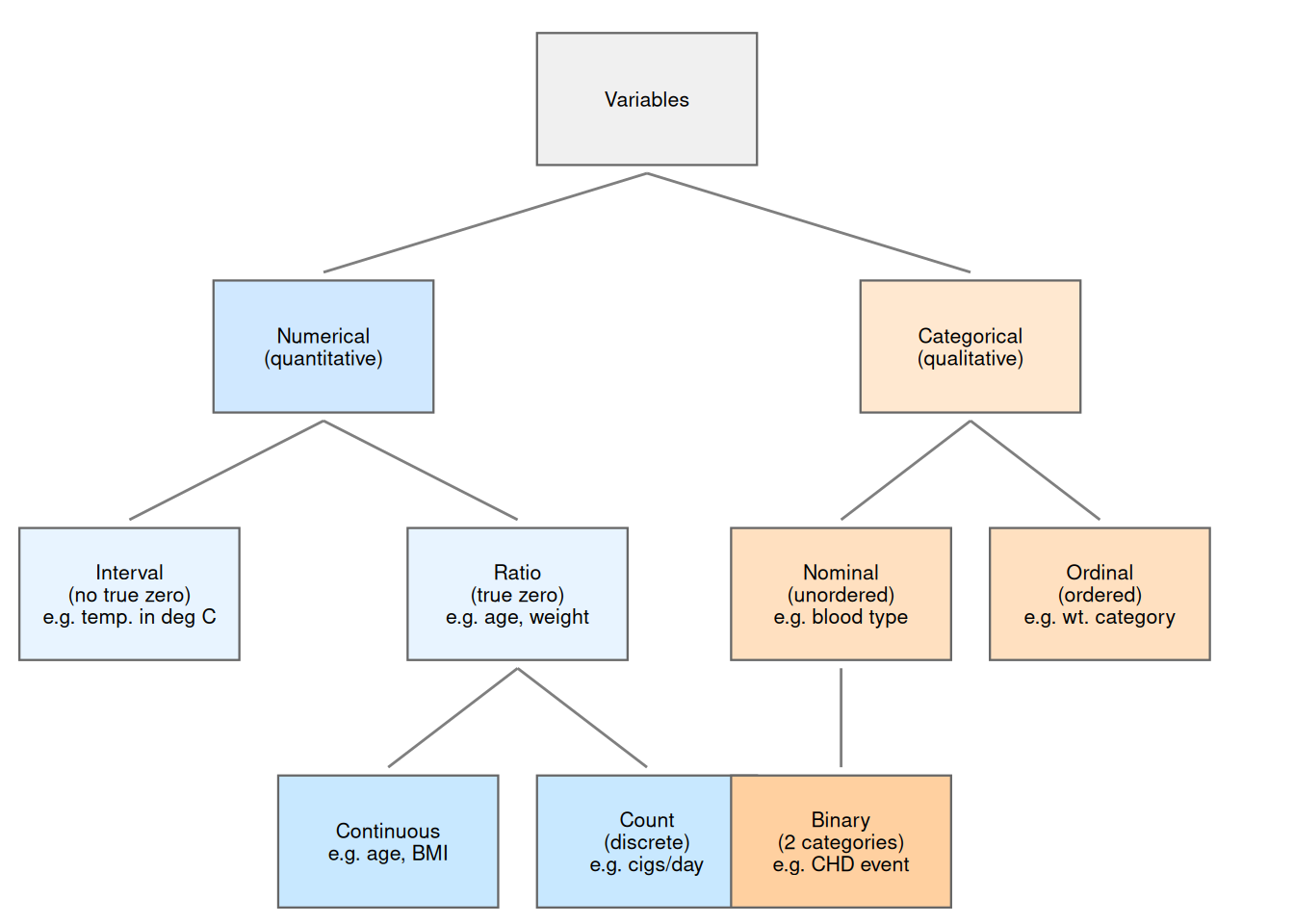
Figure 1 illustrates the relationships among these variable types.

nodes <- tibble::tribble(
  ~id,   ~x,    ~y,   ~label,
  "V",    5,    4.5,  "Variables",
  "N",    2.5,  3,    "Numerical\n(quantitative)",
  "C",    7.5,  3,    "Categorical\n(qualitative)",
  "I",    1,    1.5,  "Interval\n(no true zero)\ne.g. temp. in deg C",
  "R",    4,    1.5,  "Ratio\n(true zero)\ne.g. age, weight",
  "CT",   3,    0,    "Continuous\ne.g. age, BMI",
  "CNT",  5,    0,    "Count\n(discrete)\ne.g. cigs/day",
  "NOM",  6.5,  1.5,  "Nominal\n(unordered)\ne.g. blood type",
  "ORD",  8.5,  1.5,  "Ordinal\n(ordered)\ne.g. wt. category",
  "BIN",  6.5,  0,    "Binary\n(2 categories)\ne.g. CHD event"
)
edges <- tibble::tribble(
  ~from, ~to,
  "V",   "N",
  "V",   "C",
  "N",   "I",
  "N",   "R",
  "R",   "CT",
  "R",   "CNT",
  "C",   "NOM",
  "C",   "ORD",
  "NOM", "BIN"
) |>
  dplyr::left_join(
    dplyr::select(nodes, id, x, y),
    by = c("from" = "id")
  ) |>
  dplyr::rename(x_from = x, y_from = y) |>
  dplyr::left_join(
    dplyr::select(nodes, id, x, y),
    by = c("to" = "id")
  ) |>
  dplyr::rename(x_to = x, y_to = y)
fill_colors <- c(
  "V" = "#f0f0f0",
  "N" = "#d0e8ff", "C" = "#ffe8d0",
  "I" = "#e8f4ff", "R" = "#e8f4ff",
  "CT" = "#c8e8ff", "CNT" = "#c8e8ff",
  "NOM" = "#ffe0c0", "ORD" = "#ffe0c0",
  "BIN" = "#ffd0a0"
)
ggplot2::ggplot() +
  ggplot2::aes() +
  ggplot2::geom_segment(
    data = edges,
    ggplot2::aes(
      x = x_from, y = y_from - 0.45,
      xend = x_to, yend = y_to + 0.45
    ),
    color = "grey50"
  ) +
  ggplot2::geom_tile(
    data = nodes,
    ggplot2::aes(x = x, y = y, fill = id),
    width = 1.7, height = 0.8,
    color = "grey40", linewidth = 0.4,
    show.legend = FALSE
  ) +
  ggplot2::geom_text(
    data = nodes,
    ggplot2::aes(x = x, y = y, label = label),
    size = 2.8, lineheight = 0.9
  ) +
  ggplot2::scale_fill_manual(values = fill_colors) +
  ggplot2::scale_y_continuous(
    limits = c(-0.5, 5.1), expand = c(0, 0)
  ) +
  ggplot2::scale_x_continuous(
    limits = c(0, 10), expand = c(0, 0)
  ) +
  ggplot2::theme_void()

Figure 1: Taxonomy of variable types. Count variables are discrete and numerical; binary, nominal, and ordinal variables are discrete and categorical.

Note

The continuous/discrete distinction cuts across the numerical/categorical distinction. Continuous variables are always numerical. Discrete variables include both numerical types (such as count variables) and categorical types (such as binary, nominal, and ordinal variables).

4 Variables in the WCGS dataset

Table 1 shows selected variables from the Western Collaborative Group Study (WCGS) dataset and their types.

tibble::tribble(
  ~Variable, ~Description, ~Type, ~Scale,
  "`age`", "Age (years)", "Continuous", "Ratio",
  "`chol`", "Total cholesterol", "Continuous", "Ratio",
  "`sbp`", "Systolic blood pressure", "Continuous", "Ratio",
  "`bmi`", "Body mass index (kg/m^2)", "Continuous", "Ratio",
  "`weight`", "Weight (lbs)", "Continuous", "Ratio",
  "`ncigs`", "Cigarettes per day", "Count (discrete)", "Ratio",
  "`chd69`", "CHD event by 1969", "Binary (nominal)", "Nominal",
  "`smoke`", "Current smoking", "Binary (nominal)", "Nominal",
  "`arcus`", "Arcus senilis", "Binary (nominal)", "Nominal",
  "`dibpat`", "Behavioral pattern (A/B)", "Binary (nominal)", "Nominal",
  "`behpat`", "Behavioral pattern (A1/A2/B3/B4)", "Nominal", "Nominal",
  "`wghtcat`", "Weight category", "Ordinal", "Ordinal",
  "`agec`", "Age group", "Ordinal", "Ordinal"
) |>
  knitr::kable()

Table 1: Selected WCGS variables and their types

Selected WCGS variables and their types

Variable	Description	Type	Scale
age	Age (years)	Continuous	Ratio
chol	Total cholesterol	Continuous	Ratio
sbp	Systolic blood pressure	Continuous	Ratio
bmi	Body mass index (kg/m^2)	Continuous	Ratio
weight	Weight (lbs)	Continuous	Ratio
ncigs	Cigarettes per day	Count (discrete)	Ratio
chd69	CHD event by 1969	Binary (nominal)	Nominal
smoke	Current smoking	Binary (nominal)	Nominal
arcus	Arcus senilis	Binary (nominal)	Nominal
dibpat	Behavioral pattern (A/B)	Binary (nominal)	Nominal
behpat	Behavioral pattern (A1/A2/B3/B4)	Nominal	Nominal
wghtcat	Weight category	Ordinal	Ordinal
agec	Age group	Ordinal	Ordinal

5 Random variables

5.1 Binary variables

Definition 13 (Binary random variable) A binary variable is a random variable which has only two possible values in its range.

Exercise 2 (Examples of binary variables) What are some examples of binary variables in health sciences and data science?

SolutionSolution

Solution 2. Examples of binary outcomes include:

• exposure (exposed vs unexposed)
• disease status (diseased vs healthy)
• recovery (recovered vs unrecovered)
• relapse (relapse vs remission)
• return to hospital (returned vs not returned)
• vital status (dead vs alive)

5.2 Count variables

Definition 14 (Count variable) A count variable is a random variable whose possible values are some subset of the non-negative integers; specifically, a random variable \(X\) such that:

\[\mathcal{R}(X) \subseteq \mathbb{N}\]

Exercise 3 (Examples of count variables) What are some examples of count variables?

SolutionSolution

Solution 3. Examples of count variables include:

• number of fish in a pond
• number of cyclones per season
• seconds of tooth-brushing per session (when rounded)
• infections per person-year
• visits to an emergency room per person-month
• car accidents per 1,000 miles driven

5.2.1 Probability distributions for count outcomes

Standard probability distributions for count outcomes include:

• Poisson distribution
• Negative binomial distribution

References

Dobson, Annette J, and Adrian G Barnett. 2018. An Introduction to Generalized Linear Models. 4th ed. CRC press. https://doi.org/10.1201/9781315182780.