Poisson Regression
1 The model
A count outcome, such as the number of bike rentals in an hour, is not well described by a normal distribution when the counts are small, since the normal distribution puts probability below zero, and a count is never below zero. A Poisson regression model takes the event rate to be the exponential function of a linear function of the covariates.
DefDefinition 1 (Poisson regression model)
Definition 1 (Poisson regression model) Let \(Y\) be a count outcome, \(\mathord{\smash[b]{\underset{\raise.3ex\hbox{$\scriptstyle\sim$}}{X}}\vphantom{X}}\) a covariate vector, and \(T\) the exposure magnitude over which the events in \(Y\) are counted. A Poisson regression model assumes that, given \(\mathord{\smash[b]{\underset{\raise.3ex\hbox{$\scriptstyle\sim$}}{X}}\vphantom{X}}= \mathord{\smash[b]{\underset{\raise.3ex\hbox{$\scriptstyle\sim$}}{x}}\vphantom{x}}\) and \(T = t\), \(Y\) has a Poisson distribution with mean \(\mu(\mathord{\smash[b]{\underset{\raise.3ex\hbox{$\scriptstyle\sim$}}{x}}\vphantom{x}}, t) = \lambda(\mathord{\smash[b]{\underset{\raise.3ex\hbox{$\scriptstyle\sim$}}{x}}\vphantom{x}}) \cdot t\), where the event rate \(\lambda(\mathord{\smash[b]{\underset{\raise.3ex\hbox{$\scriptstyle\sim$}}{x}}\vphantom{x}})\) has a log that is a linear function of the covariates:
\[ {\ln\mathopen{}\left(\lambda(\mathord{\smash[b]{\underset{\raise.3ex\hbox{$\scriptstyle\sim$}}{x}}\vphantom{x}})\right)\mathclose{}} = \beta_0 + \beta_1 x_1 + \ldots+ \beta_p x_p. \]
2 Rate ratios
DefDefinition 2 (Rate ratio)
Definition 2 (Rate ratio) In a Poisson regression model, the rate ratio comparing covariate pattern \(\mathord{\smash[b]{\underset{\raise.3ex\hbox{$\scriptstyle\sim$}}{x}}\vphantom{x}}\) to covariate pattern \(\mathord{{\mathord{\smash[b]{\underset{\raise.3ex\hbox{$\scriptstyle\sim$}}{x}}\vphantom{x}}^*}}\) is the ratio of their event rates:
\[\text{ϙ}_{{\lambda}}(\mathord{\smash[b]{\underset{\raise.3ex\hbox{$\scriptstyle\sim$}}{x}}\vphantom{x}}: \mathord{{\mathord{\smash[b]{\underset{\raise.3ex\hbox{$\scriptstyle\sim$}}{x}}\vphantom{x}}^*}}) \stackrel{\text{def}}{=}\frac{\lambda(\mathord{\smash[b]{\underset{\raise.3ex\hbox{$\scriptstyle\sim$}}{x}}\vphantom{x}})}{\lambda(\mathord{{\mathord{\smash[b]{\underset{\raise.3ex\hbox{$\scriptstyle\sim$}}{x}}\vphantom{x}}^*}})}.\]
LemTheorem 1 (Rate ratios in Poisson regression)
Theorem 1 (Rate ratios in Poisson regression) In a Poisson regression model, suppose covariate \(x_j\) enters the linear function \({\ln\mathopen{}\left(\lambda(\mathord{\smash[b]{\underset{\raise.3ex\hbox{$\scriptstyle\sim$}}{x}}\vphantom{x}})\right)\mathclose{}}\) only through the single term \(\beta_j x_j\) (no interactions or transformations involving \(x_j\)). Let \(\mathord{\smash[b]{\underset{\raise.3ex\hbox{$\scriptstyle\sim$}}{x}}\vphantom{x}}\) and \(\mathord{{\mathord{\smash[b]{\underset{\raise.3ex\hbox{$\scriptstyle\sim$}}{x}}\vphantom{x}}^*}}\) be two covariate patterns that are identical except that \(x_j = a\) and \(x^*_j = b\). Then
\[\text{ϙ}_{{\lambda}}(\mathord{\smash[b]{\underset{\raise.3ex\hbox{$\scriptstyle\sim$}}{x}}\vphantom{x}}: \mathord{{\mathord{\smash[b]{\underset{\raise.3ex\hbox{$\scriptstyle\sim$}}{x}}\vphantom{x}}^*}}) = {\operatorname{exp}\mathopen{}\left\{\beta_j (a - b)\right\}\mathclose{}} \tag{1}\]
and for any common exposure magnitude \(t > 0\), the ratio of the means is the same rate ratio:
\[\frac{\mu(\mathord{\smash[b]{\underset{\raise.3ex\hbox{$\scriptstyle\sim$}}{x}}\vphantom{x}}, t)}{\mu(\mathord{{\mathord{\smash[b]{\underset{\raise.3ex\hbox{$\scriptstyle\sim$}}{x}}\vphantom{x}}^*}}, t)} = \text{ϙ}_{{\lambda}}(\mathord{\smash[b]{\underset{\raise.3ex\hbox{$\scriptstyle\sim$}}{x}}\vphantom{x}}: \mathord{{\mathord{\smash[b]{\underset{\raise.3ex\hbox{$\scriptstyle\sim$}}{x}}\vphantom{x}}^*}})\]
ProofProof
Proof. Because \(\mathord{\smash[b]{\underset{\raise.3ex\hbox{$\scriptstyle\sim$}}{x}}\vphantom{x}}\) and \(\mathord{{\mathord{\smash[b]{\underset{\raise.3ex\hbox{$\scriptstyle\sim$}}{x}}\vphantom{x}}^*}}\) agree on every covariate except \(x_j\), every term of \({\ln\mathopen{}\left(\lambda(\mathord{\smash[b]{\underset{\raise.3ex\hbox{$\scriptstyle\sim$}}{x}}\vphantom{x}})\right)\mathclose{}}\) except \(\beta_j x_j\) is shared with \({\ln\mathopen{}\left(\lambda(\mathord{{\mathord{\smash[b]{\underset{\raise.3ex\hbox{$\scriptstyle\sim$}}{x}}\vphantom{x}}^*}})\right)\mathclose{}}\):
\[ \begin{aligned} {\ln\mathopen{}\left(\lambda(\mathord{\smash[b]{\underset{\raise.3ex\hbox{$\scriptstyle\sim$}}{x}}\vphantom{x}})\right)\mathclose{}} - {\ln\mathopen{}\left(\lambda(\mathord{{\mathord{\smash[b]{\underset{\raise.3ex\hbox{$\scriptstyle\sim$}}{x}}\vphantom{x}}^*}})\right)\mathclose{}} &= \mathopen{}\left(\beta_0 + \beta_1 x_1 + \ldots+ {\color{red}{\beta_j a}} + \ldots+ \beta_p x_p\right)\mathclose{} \\ &\phantom{={}} - \mathopen{}\left(\beta_0 + \beta_1 x_1 + \ldots+ {\color{red}{\beta_j b}} + \ldots+ \beta_p x_p\right)\mathclose{} && \text{(substitute the linear function)} \\ &= {\color{red}{\beta_j a}} - {\color{red}{\beta_j b}} && \text{(cancel the shared terms)} \\ &= {\color{red}{\beta_j (a - b)}} && \text{(factor out } \beta_j \text{)} \end{aligned} \]
Then the rate ratio is:
\[ \begin{aligned} \text{ϙ}_{{\lambda}}(\mathord{\smash[b]{\underset{\raise.3ex\hbox{$\scriptstyle\sim$}}{x}}\vphantom{x}}: \mathord{{\mathord{\smash[b]{\underset{\raise.3ex\hbox{$\scriptstyle\sim$}}{x}}\vphantom{x}}^*}}) &= \frac{\lambda(\mathord{\smash[b]{\underset{\raise.3ex\hbox{$\scriptstyle\sim$}}{x}}\vphantom{x}})}{\lambda(\mathord{{\mathord{\smash[b]{\underset{\raise.3ex\hbox{$\scriptstyle\sim$}}{x}}\vphantom{x}}^*}})} && \text{(definition of rate ratio)} \\ &= \frac{{\operatorname{exp}\mathopen{}\left\{{\ln\mathopen{}\left(\lambda(\mathord{\smash[b]{\underset{\raise.3ex\hbox{$\scriptstyle\sim$}}{x}}\vphantom{x}})\right)\mathclose{}}\right\}\mathclose{}}}{{\operatorname{exp}\mathopen{}\left\{{\ln\mathopen{}\left(\lambda(\mathord{{\mathord{\smash[b]{\underset{\raise.3ex\hbox{$\scriptstyle\sim$}}{x}}\vphantom{x}}^*}})\right)\mathclose{}}\right\}\mathclose{}}} && \text{(exponential undoes the log)} \\ &= {\operatorname{exp}\mathopen{}\left\{{\ln\mathopen{}\left(\lambda(\mathord{\smash[b]{\underset{\raise.3ex\hbox{$\scriptstyle\sim$}}{x}}\vphantom{x}})\right)\mathclose{}} - {\ln\mathopen{}\left(\lambda(\mathord{{\mathord{\smash[b]{\underset{\raise.3ex\hbox{$\scriptstyle\sim$}}{x}}\vphantom{x}}^*}})\right)\mathclose{}}\right\}\mathclose{}} && \text{(quotient rule for exponentials)} \\ &= {\operatorname{exp}\mathopen{}\left\{\beta_j (a - b)\right\}\mathclose{}} && \text{(substitute the difference of linear functions)} \end{aligned} \]
For the means at a common exposure \(t > 0\):
\[ \begin{aligned} \frac{\mu(\mathord{\smash[b]{\underset{\raise.3ex\hbox{$\scriptstyle\sim$}}{x}}\vphantom{x}}, t)}{\mu(\mathord{{\mathord{\smash[b]{\underset{\raise.3ex\hbox{$\scriptstyle\sim$}}{x}}\vphantom{x}}^*}}, t)} &= \frac{\lambda(\mathord{\smash[b]{\underset{\raise.3ex\hbox{$\scriptstyle\sim$}}{x}}\vphantom{x}}) \cdot t}{\lambda(\mathord{{\mathord{\smash[b]{\underset{\raise.3ex\hbox{$\scriptstyle\sim$}}{x}}\vphantom{x}}^*}}) \cdot t} && \text{(Poisson regression mean function)} \\ &= \frac{\lambda(\mathord{\smash[b]{\underset{\raise.3ex\hbox{$\scriptstyle\sim$}}{x}}\vphantom{x}})}{\lambda(\mathord{{\mathord{\smash[b]{\underset{\raise.3ex\hbox{$\scriptstyle\sim$}}{x}}\vphantom{x}}^*}})} && \text{(cancel } t > 0 \text{)} \\ &= \text{ϙ}_{{\lambda}}(\mathord{\smash[b]{\underset{\raise.3ex\hbox{$\scriptstyle\sim$}}{x}}\vphantom{x}}: \mathord{{\mathord{\smash[b]{\underset{\raise.3ex\hbox{$\scriptstyle\sim$}}{x}}\vphantom{x}}^*}}) && \text{(definition of rate ratio)} \end{aligned} \]
ExmExample 1 (Rate ratio for a ten-year age difference)
Example 1 (Rate ratio for a ten-year age difference)
Suppose a Poisson regression model for emergency-room visits includes age in years, \(x_1\), with coefficient \(\beta_1 = 0.03\) and no interactions involving age. By Theorem 1 with \(a = 60\) and \(b = 50\), the rate ratio comparing a 60-year-old to a 50-year-old with the same values of every other covariate is:
\[ \begin{aligned} \text{ϙ}_{{\lambda}}(x_1 = 60 : x_1 = 50) &= {\operatorname{exp}\mathopen{}\left\{\beta_1 (60 - 50)\right\}\mathclose{}} && \text{(rate ratio theorem)} \\ &= {\operatorname{exp}\mathopen{}\left\{0.03 \cdot 10\right\}\mathclose{}} && \text{(substitute } \beta_1 \text{ and subtract)} \\ &= {\operatorname{exp}\mathopen{}\left\{0.3\right\}\mathclose{}} && \text{(multiply)} \\ &\approx 1.350 && \text{(evaluate)} \end{aligned} \]
A one-year age difference instead gives \({\operatorname{exp}\mathopen{}\left\{0.03\right\}\mathclose{}} \approx 1.030\), a 3% higher event rate per year of age. The ten-year rate ratio is the one-year rate ratio multiplied by itself ten times, \({\operatorname{exp}\mathopen{}\left\{0.3\right\}\mathclose{}} = \mathopen{}\left({\operatorname{exp}\mathopen{}\left\{0.03\right\}\mathclose{}}\right)\mathclose{}^{10}\), because rate ratios multiply across successive one-year steps.
3 Lab: Poisson regression on bike rentals
Hourly counts of bikes rented in a bike-sharing program in Washington, D.C., on 8645 hours make up the Bikeshare data [1, Sec. 4.6.2]. The data are in data/bikeshare.csv, one line per hour, copied from the book’s ISLR2 R package. The exercises use these variables:
-
bikers: the outcome, the number of bikes rented in that hour. -
temp: the temperature, scaled to run from \(0\) to \(1\). -
workingday:1on a working day and0otherwise. -
weathersit: the weather, one ofclear,cloudy/misty,light rain/snow, andheavy rain/snow.
Show code
import pandas as pd

# The first rows of the four columns that the exercises use.
bikeshare_raw = pd.read_csv("data/bikeshare.csv")
bikeshare_raw[["bikers", "temp", "workingday", "weathersit"]].head(6)
#>    bikers  temp  workingday    weathersit
#> 0      16  0.24           0         clear
#> 1      40  0.22           0         clear
#> 2      32  0.22           0         clear
#> 3      13  0.24           0         clear
#> 4       1  0.24           0         clear
#> 5       1  0.24           0  cloudy/misty
The exercises follow the Poisson regression part of the book’s Chapter 4 lab [1, Sec. 4.7.7]. Each solution shows the code in R and in Python. Where R code without the tidyverse would differ, an R (base) tab follows the R tab, which uses the tidyverse.
ExrExercise 1 (The average hourly count of bike rentals)
ExrExercise 2 (The weather with the most rentals)
ExrExercise 3 (A histogram of the hourly count)
SolutionSolution 3
Solution 3.
Show code
bikeshare_raw |>
  ggplot2::ggplot() +
  ggplot2::aes(x = bikers) +
  ggplot2::geom_histogram(bins = 30) + # check-unexplained-choices: allow
  ggplot2::labs(x = "Bikes rented in the hour", y = "Number of hours")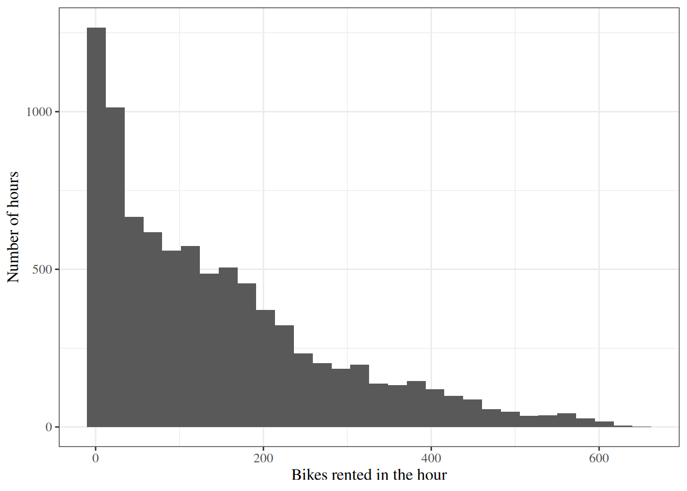
Show code
# 30 bars of equal width, from the smallest count to the largest.
bikers_range <- range(bikeshare_raw$bikers)
bikers_breaks <- seq(
  bikers_range[1],
  bikers_range[2],
  length.out = 31 # check-unexplained-choices: allow
)
hist(
  bikeshare_raw$bikers,
  breaks = bikers_breaks, # check-unexplained-choices: allow
  main = NULL,
  xlab = "Bikes rented in the hour",
  ylab = "Number of hours"
)
Show code
import matplotlib.pyplot as plt

fig, ax = plt.subplots(figsize=(6, 4), layout="constrained")
ax.hist(bikeshare_raw["bikers"], bins=30);  # check-unexplained-choices: allow
ax.set_xlabel("Bikes rented in the hour");
ax.set_ylabel("Number of hours");
plt.show()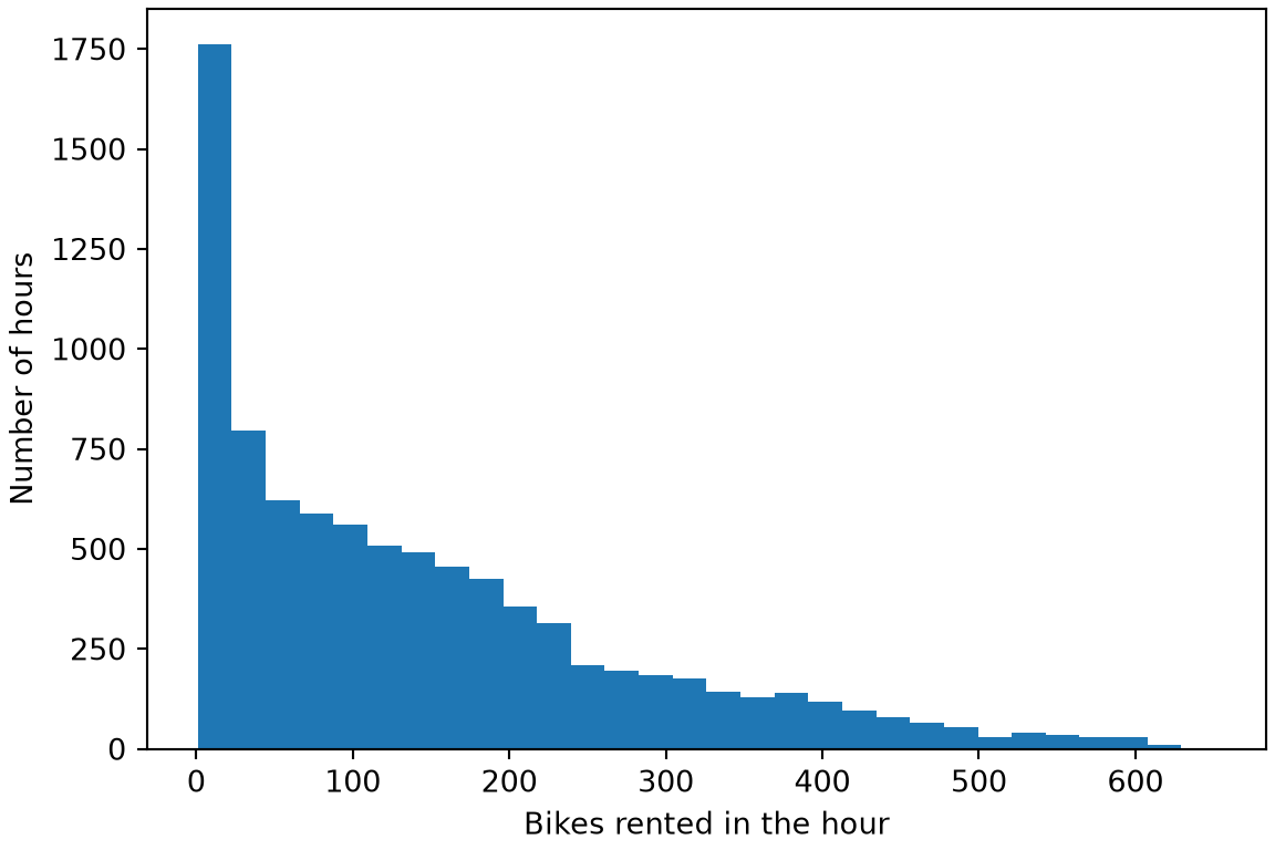
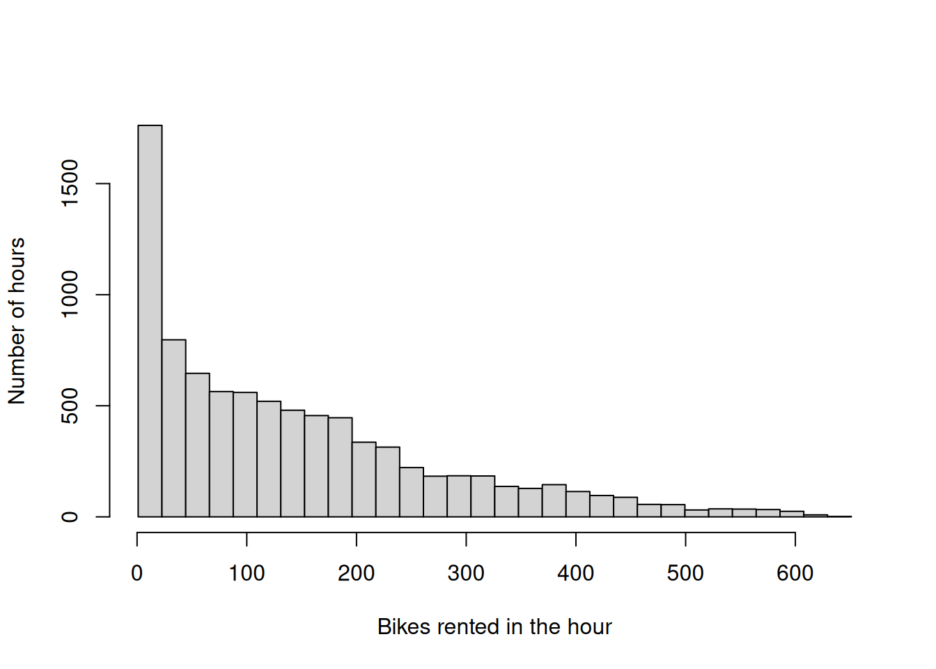
I chose 30 bars, which is about 288 hours per bar. Far fewer bars would hide the long right tail inside a few wide bars, and far more would leave most bars with only a few hours, so the outline would look ragged.
The histogram is right-skewed: the sample median of bikers is 109, below its sample mean of 143.8. Counts cannot be negative, and nothing caps them, which is the situation that a Poisson regression model is built for.
ExrExercise 4 (Rentals against temperature)
SolutionSolution 4
Solution 4.
Show code
# Small, faint points, because thousands of hours overlap.
bikeshare_raw |>
  ggplot2::ggplot() +
  ggplot2::aes(x = temp, y = bikers) +
  ggplot2::geom_point(size = 0.5, alpha = 0.3) +
  ggplot2::labs(
    x = "Temperature (scaled to 0 to 1)",
    y = "Bikes rented in the hour"
  )
Show code
# Small, faint points, because thousands of hours overlap.
faint_black <- grDevices::adjustcolor("black", alpha.f = 0.3)
plot(
  bikeshare_raw$temp,
  bikeshare_raw$bikers,
  pch = 16,
  cex = 0.3,
  col = faint_black,
  xlab = "Temperature (scaled to 0 to 1)",
  ylab = "Bikes rented in the hour"
)
Show code
# Small, faint points, because thousands of hours overlap.
fig, ax = plt.subplots(figsize=(6, 4), layout="constrained")
ax.scatter(bikeshare_raw["temp"], bikeshare_raw["bikers"], s=4, alpha=0.3);
ax.set_xlabel("Temperature (scaled to 0 to 1)");
ax.set_ylabel("Bikes rented in the hour");
plt.show()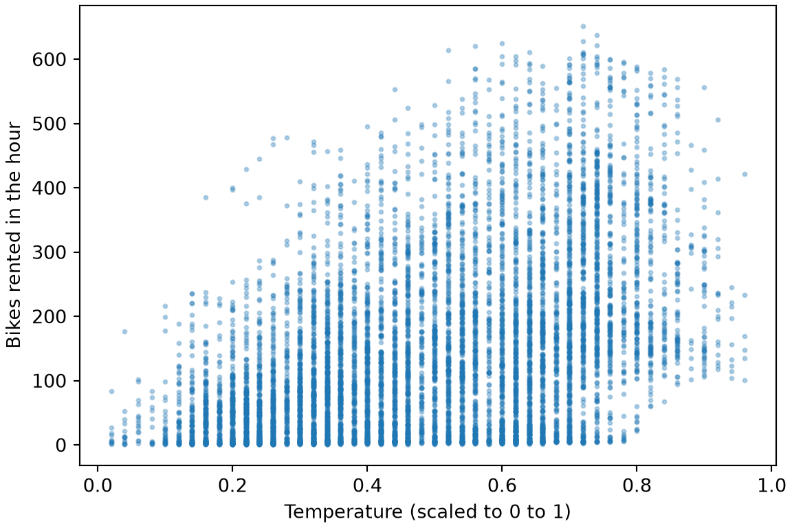
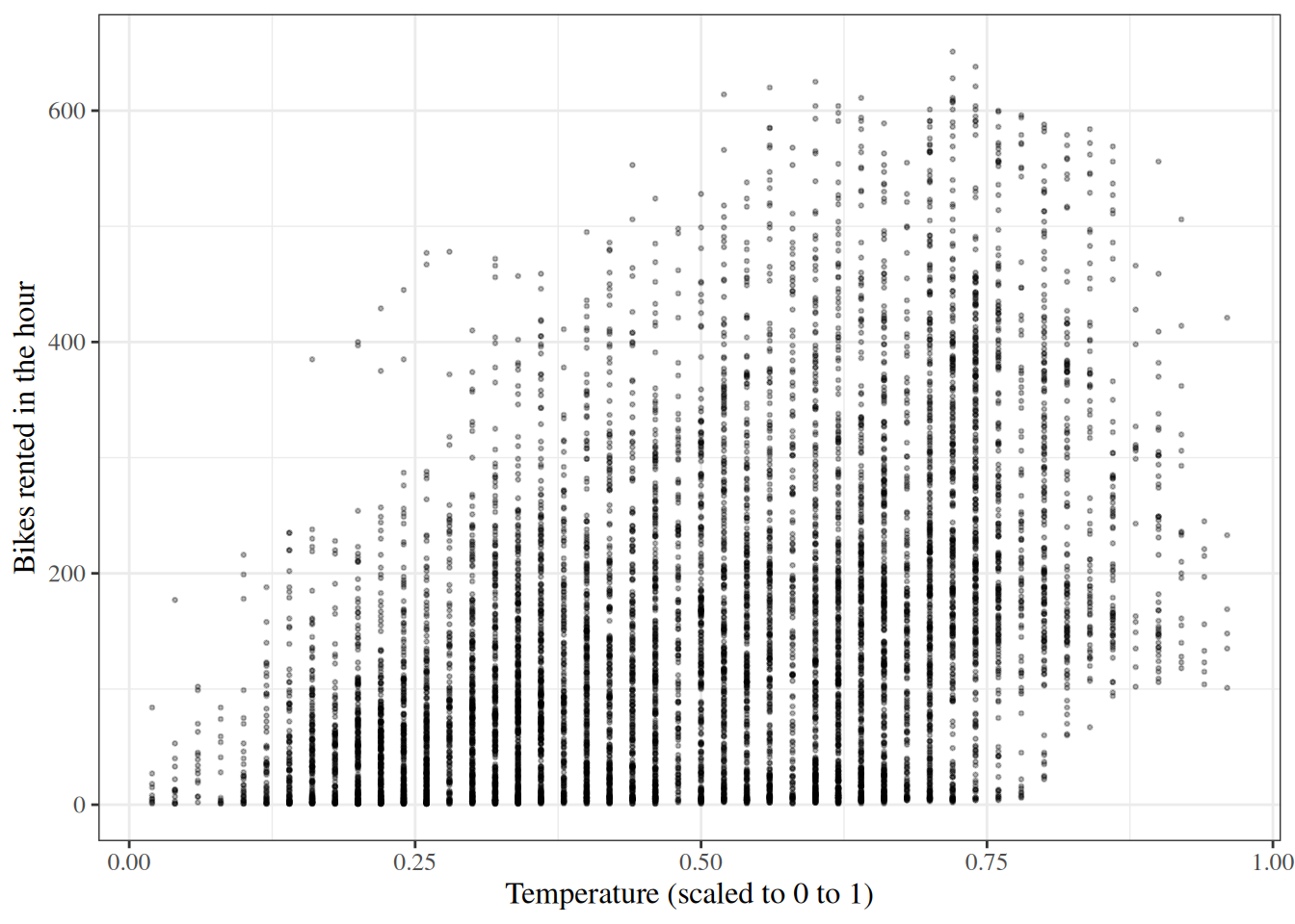
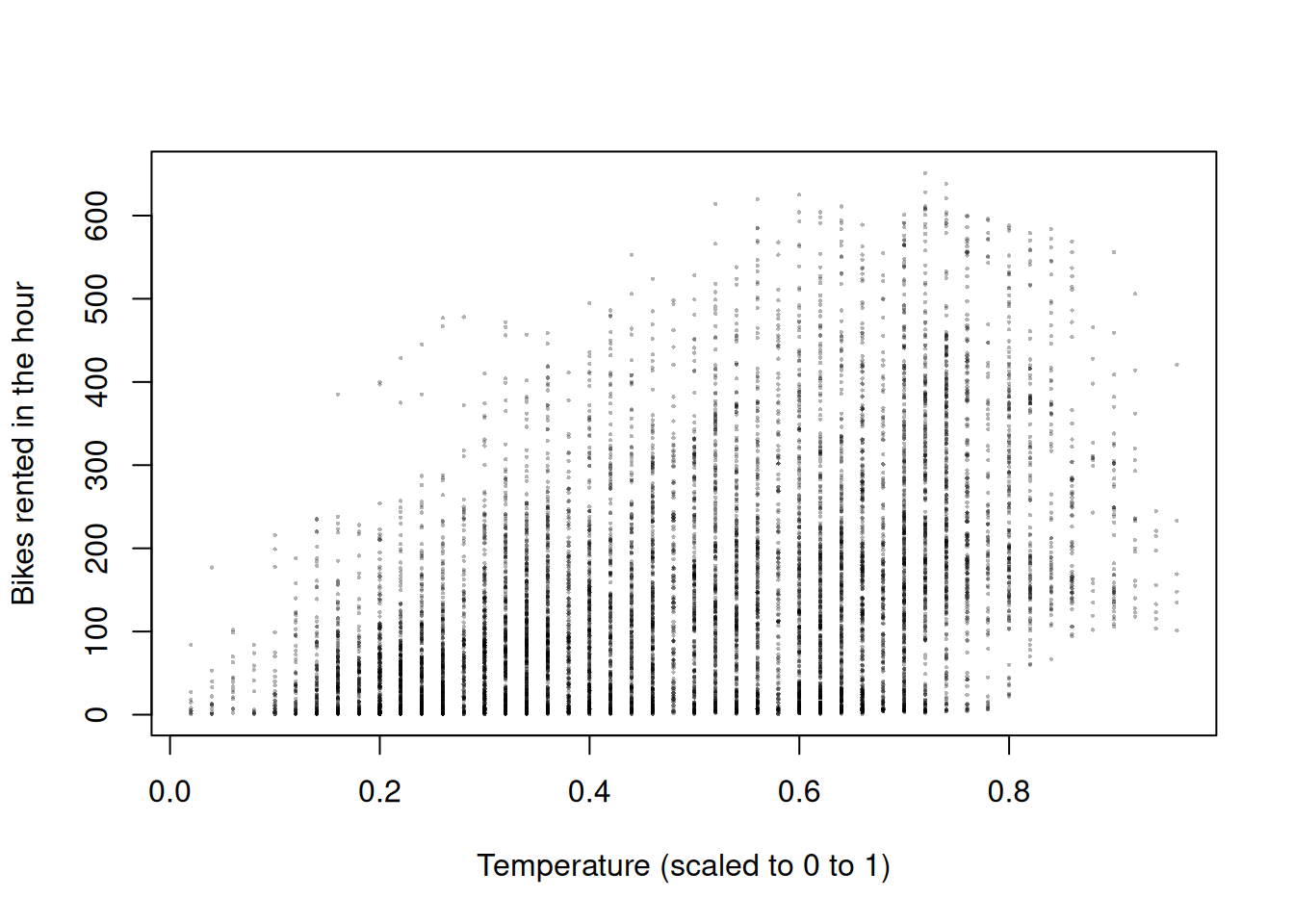
The counts rise with the temperature, with sample correlation 0.45. The spread of the counts grows with their level. A Poisson regression model describes that pattern, because the variance of a Poisson variable is the same as its expected value.
ExrExercise 5 (Fit a Poisson regression to bike rentals)
ExrExercise 6 (Interpret the temperature coefficient)
ExrExercise 7 (Compare with linear regression)
Definitions on this page
References
[1]
G. James, D. Witten, T. Hastie, and R. Tibshirani, An introduction to statistical learning: With applications in R, 2nd ed. Springer, 2021. doi: 10.1007/978-1-0716-1418-1.