Poisson Regression
Last modified: 2026-11-20 00:37:14 (PST)
1 The model
A count outcome, such as the number of bike rentals in an hour, is not well described by a normal distribution when the counts are small, since the normal distribution puts probability below zero, and a count is never below zero. A Poisson regression model takes the event rate to be the exponential function of a linear function of the covariates.
Definition 1 (Poisson regression model) Let \(Y\) be a count outcome, \(\mathord{\smash[b]{\underset{\raise.3ex\hbox{$\scriptstyle\sim$}}{X}}\vphantom{X}}\) a covariate vector, and \(T\) the exposure magnitude over which the events in \(Y\) are counted. A Poisson regression model assumes that, given \(\mathord{\smash[b]{\underset{\raise.3ex\hbox{$\scriptstyle\sim$}}{X}}\vphantom{X}}= \mathord{\smash[b]{\underset{\raise.3ex\hbox{$\scriptstyle\sim$}}{x}}\vphantom{x}}\) and \(T = t\), \(Y\) has a Poisson distribution with mean \(\mu(\mathord{\smash[b]{\underset{\raise.3ex\hbox{$\scriptstyle\sim$}}{x}}\vphantom{x}}, t) = \lambda(\mathord{\smash[b]{\underset{\raise.3ex\hbox{$\scriptstyle\sim$}}{x}}\vphantom{x}}) \cdot t\), where the event rate \(\lambda(\mathord{\smash[b]{\underset{\raise.3ex\hbox{$\scriptstyle\sim$}}{x}}\vphantom{x}})\) has a log that is a linear function of the covariates:
\[ {\ln\mathopen{}\left(\lambda(\mathord{\smash[b]{\underset{\raise.3ex\hbox{$\scriptstyle\sim$}}{x}}\vphantom{x}})\right)\mathclose{}} = \beta_0 + \beta_1 x_1 + \ldots+ \beta_p x_p. \]
2 Rate ratios
Definition 2 (Rate ratio) In a Poisson regression model, the rate ratio comparing covariate pattern \(\mathord{\smash[b]{\underset{\raise.3ex\hbox{$\scriptstyle\sim$}}{x}}\vphantom{x}}\) to covariate pattern \(\mathord{{\mathord{\smash[b]{\underset{\raise.3ex\hbox{$\scriptstyle\sim$}}{x}}\vphantom{x}}^*}}\) is the ratio of their event rates:
\[\text{ϙ}_{{\lambda}}(\mathord{\smash[b]{\underset{\raise.3ex\hbox{$\scriptstyle\sim$}}{x}}\vphantom{x}}: \mathord{{\mathord{\smash[b]{\underset{\raise.3ex\hbox{$\scriptstyle\sim$}}{x}}\vphantom{x}}^*}}) \stackrel{\text{def}}{=}\frac{\lambda(\mathord{\smash[b]{\underset{\raise.3ex\hbox{$\scriptstyle\sim$}}{x}}\vphantom{x}})}{\lambda(\mathord{{\mathord{\smash[b]{\underset{\raise.3ex\hbox{$\scriptstyle\sim$}}{x}}\vphantom{x}}^*}})}.\]
Theorem 1 (Rate ratios in Poisson regression) In a Poisson regression model, suppose covariate \(x_j\) enters the linear function \({\ln\mathopen{}\left(\lambda(\mathord{\smash[b]{\underset{\raise.3ex\hbox{$\scriptstyle\sim$}}{x}}\vphantom{x}})\right)\mathclose{}}\) only through the single term \(\beta_j x_j\) (no interactions or transformations involving \(x_j\)). Let \(\mathord{\smash[b]{\underset{\raise.3ex\hbox{$\scriptstyle\sim$}}{x}}\vphantom{x}}\) and \(\mathord{{\mathord{\smash[b]{\underset{\raise.3ex\hbox{$\scriptstyle\sim$}}{x}}\vphantom{x}}^*}}\) be two covariate patterns that are identical except that \(x_j = a\) and \(x^*_j = b\). Then
\[\text{ϙ}_{{\lambda}}(\mathord{\smash[b]{\underset{\raise.3ex\hbox{$\scriptstyle\sim$}}{x}}\vphantom{x}}: \mathord{{\mathord{\smash[b]{\underset{\raise.3ex\hbox{$\scriptstyle\sim$}}{x}}\vphantom{x}}^*}}) = {\operatorname{exp}\mathopen{}\left\{\beta_j (a - b)\right\}\mathclose{}} \tag{1}\]
and for any common exposure magnitude \(t > 0\), the ratio of the means is the same rate ratio:
\[\frac{\mu(\mathord{\smash[b]{\underset{\raise.3ex\hbox{$\scriptstyle\sim$}}{x}}\vphantom{x}}, t)}{\mu(\mathord{{\mathord{\smash[b]{\underset{\raise.3ex\hbox{$\scriptstyle\sim$}}{x}}\vphantom{x}}^*}}, t)} = \text{ϙ}_{{\lambda}}(\mathord{\smash[b]{\underset{\raise.3ex\hbox{$\scriptstyle\sim$}}{x}}\vphantom{x}}: \mathord{{\mathord{\smash[b]{\underset{\raise.3ex\hbox{$\scriptstyle\sim$}}{x}}\vphantom{x}}^*}})\]
Proof. Because \(\mathord{\smash[b]{\underset{\raise.3ex\hbox{$\scriptstyle\sim$}}{x}}\vphantom{x}}\) and \(\mathord{{\mathord{\smash[b]{\underset{\raise.3ex\hbox{$\scriptstyle\sim$}}{x}}\vphantom{x}}^*}}\) agree on every covariate except \(x_j\), every term of \({\ln\mathopen{}\left(\lambda(\mathord{\smash[b]{\underset{\raise.3ex\hbox{$\scriptstyle\sim$}}{x}}\vphantom{x}})\right)\mathclose{}}\) except \(\beta_j x_j\) is shared with \({\ln\mathopen{}\left(\lambda(\mathord{{\mathord{\smash[b]{\underset{\raise.3ex\hbox{$\scriptstyle\sim$}}{x}}\vphantom{x}}^*}})\right)\mathclose{}}\):
\[ \begin{aligned} {\ln\mathopen{}\left(\lambda(\mathord{\smash[b]{\underset{\raise.3ex\hbox{$\scriptstyle\sim$}}{x}}\vphantom{x}})\right)\mathclose{}} - {\ln\mathopen{}\left(\lambda(\mathord{{\mathord{\smash[b]{\underset{\raise.3ex\hbox{$\scriptstyle\sim$}}{x}}\vphantom{x}}^*}})\right)\mathclose{}} &= \mathopen{}\left(\beta_0 + \beta_1 x_1 + \ldots+ {\color{red}{\beta_j a}} + \ldots+ \beta_p x_p\right)\mathclose{} \\ &\phantom{={}} - \mathopen{}\left(\beta_0 + \beta_1 x_1 + \ldots+ {\color{red}{\beta_j b}} + \ldots+ \beta_p x_p\right)\mathclose{} && \text{(substitute the linear function)} \\ &= {\color{red}{\beta_j a}} - {\color{red}{\beta_j b}} && \text{(cancel the shared terms)} \\ &= {\color{red}{\beta_j (a - b)}} && \text{(factor out } \beta_j \text{)} \end{aligned} \]
Then the rate ratio is:
\[ \begin{aligned} \text{ϙ}_{{\lambda}}(\mathord{\smash[b]{\underset{\raise.3ex\hbox{$\scriptstyle\sim$}}{x}}\vphantom{x}}: \mathord{{\mathord{\smash[b]{\underset{\raise.3ex\hbox{$\scriptstyle\sim$}}{x}}\vphantom{x}}^*}}) &= \frac{\lambda(\mathord{\smash[b]{\underset{\raise.3ex\hbox{$\scriptstyle\sim$}}{x}}\vphantom{x}})}{\lambda(\mathord{{\mathord{\smash[b]{\underset{\raise.3ex\hbox{$\scriptstyle\sim$}}{x}}\vphantom{x}}^*}})} && \text{(definition of rate ratio)} \\ &= \frac{{\operatorname{exp}\mathopen{}\left\{{\ln\mathopen{}\left(\lambda(\mathord{\smash[b]{\underset{\raise.3ex\hbox{$\scriptstyle\sim$}}{x}}\vphantom{x}})\right)\mathclose{}}\right\}\mathclose{}}}{{\operatorname{exp}\mathopen{}\left\{{\ln\mathopen{}\left(\lambda(\mathord{{\mathord{\smash[b]{\underset{\raise.3ex\hbox{$\scriptstyle\sim$}}{x}}\vphantom{x}}^*}})\right)\mathclose{}}\right\}\mathclose{}}} && \text{(exponential undoes the log)} \\ &= {\operatorname{exp}\mathopen{}\left\{{\ln\mathopen{}\left(\lambda(\mathord{\smash[b]{\underset{\raise.3ex\hbox{$\scriptstyle\sim$}}{x}}\vphantom{x}})\right)\mathclose{}} - {\ln\mathopen{}\left(\lambda(\mathord{{\mathord{\smash[b]{\underset{\raise.3ex\hbox{$\scriptstyle\sim$}}{x}}\vphantom{x}}^*}})\right)\mathclose{}}\right\}\mathclose{}} && \text{(quotient rule for exponentials)} \\ &= {\operatorname{exp}\mathopen{}\left\{\beta_j (a - b)\right\}\mathclose{}} && \text{(substitute the difference of linear functions)} \end{aligned} \]
For the means at a common exposure \(t > 0\):
\[ \begin{aligned} \frac{\mu(\mathord{\smash[b]{\underset{\raise.3ex\hbox{$\scriptstyle\sim$}}{x}}\vphantom{x}}, t)}{\mu(\mathord{{\mathord{\smash[b]{\underset{\raise.3ex\hbox{$\scriptstyle\sim$}}{x}}\vphantom{x}}^*}}, t)} &= \frac{\lambda(\mathord{\smash[b]{\underset{\raise.3ex\hbox{$\scriptstyle\sim$}}{x}}\vphantom{x}}) \cdot t}{\lambda(\mathord{{\mathord{\smash[b]{\underset{\raise.3ex\hbox{$\scriptstyle\sim$}}{x}}\vphantom{x}}^*}}) \cdot t} && \text{(Poisson regression mean function)} \\ &= \frac{\lambda(\mathord{\smash[b]{\underset{\raise.3ex\hbox{$\scriptstyle\sim$}}{x}}\vphantom{x}})}{\lambda(\mathord{{\mathord{\smash[b]{\underset{\raise.3ex\hbox{$\scriptstyle\sim$}}{x}}\vphantom{x}}^*}})} && \text{(cancel } t > 0 \text{)} \\ &= \text{ϙ}_{{\lambda}}(\mathord{\smash[b]{\underset{\raise.3ex\hbox{$\scriptstyle\sim$}}{x}}\vphantom{x}}: \mathord{{\mathord{\smash[b]{\underset{\raise.3ex\hbox{$\scriptstyle\sim$}}{x}}\vphantom{x}}^*}}) && \text{(definition of rate ratio)} \end{aligned} \]
Example 1 (Rate ratio for a ten-year age difference)
Suppose a Poisson regression model for emergency-room visits includes age in years, \(x_1\), with coefficient \(\beta_1 = 0.03\) and no interactions involving age. By Theorem 1 with \(a = 60\) and \(b = 50\), the rate ratio comparing a 60-year-old to a 50-year-old with the same values of every other covariate is:
\[ \begin{aligned} \text{ϙ}_{{\lambda}}(x_1 = 60 : x_1 = 50) &= {\operatorname{exp}\mathopen{}\left\{\beta_1 (60 - 50)\right\}\mathclose{}} && \text{(rate ratio theorem)} \\ &= {\operatorname{exp}\mathopen{}\left\{0.03 \cdot 10\right\}\mathclose{}} && \text{(substitute } \beta_1 \text{ and subtract)} \\ &= {\operatorname{exp}\mathopen{}\left\{0.3\right\}\mathclose{}} && \text{(multiply)} \\ &\approx 1.350 && \text{(evaluate)} \end{aligned} \]
A one-year age difference instead gives \({\operatorname{exp}\mathopen{}\left\{0.03\right\}\mathclose{}} \approx 1.030\), a 3% higher event rate per year of age. The ten-year rate ratio is the one-year rate ratio multiplied by itself ten times, \({\operatorname{exp}\mathopen{}\left\{0.3\right\}\mathclose{}} = \mathopen{}\left({\operatorname{exp}\mathopen{}\left\{0.03\right\}\mathclose{}}\right)\mathclose{}^{10}\), because rate ratios multiply across successive one-year steps.
3 Lab: Poisson regression on bike rentals
Hourly counts of bikes rented in a bike-sharing program in Washington, D.C., on 8645 hours make up the Bikeshare data [1, Sec. 4.6.2]. The data are in data/bikeshare.csv, one line per hour, copied from the book’s ISLR2 R package. The exercises use these variables:
-
bikers: the outcome, the number of bikes rented in that hour. -
temp: the temperature, scaled to run from \(0\) to \(1\). -
workingday:1on a working day and0otherwise. -
weathersit: the weather, one ofclear,cloudy/misty,light rain/snow, andheavy rain/snow.
[Code]
import pandas as pd

# The first rows of the four columns that the exercises use.
bikeshare_raw = pd.read_csv("data/bikeshare.csv")
bikeshare_raw[["bikers", "temp", "workingday", "weathersit"]].head(6)
#>    bikers  temp  workingday    weathersit
#> 0      16  0.24           0         clear
#> 1      40  0.22           0         clear
#> 2      32  0.22           0         clear
#> 3      13  0.24           0         clear
#> 4       1  0.24           0         clear
#> 5       1  0.24           0  cloudy/misty
The exercises follow the Poisson regression part of the book’s Chapter 4 lab [1, Sec. 4.7.7]. Each solution shows the code in R and in Python. Where R code without the tidyverse would differ, an R (base) tab follows the R tab, which uses the tidyverse.
Exercise 1 (The average hourly count of bike rentals) The Bikeshare data count the bikes rented in each of many hours, as bikers. A first look at a count outcome starts with its typical size.
Hint
mean() in R and the pandas .mean() method in Python compute a sample mean.
Compute the sample mean of bikers.
Solution 1.
The sample mean of bikers is 143.8 bikes per hour. A Poisson regression model with no covariates would estimate the expected hourly count by this sample mean.
Exercise 2 (The weather with the most rentals) The Bikeshare data record the weather of each hour as weathersit, and the number of bikes rented in that hour as bikers. A covariate whose groups have very different sample means of the outcome is a promising one for a regression model.
Hint
dplyr::group_by() and dplyr::summarise() in R, tapply() in R without the tidyverse, and the .groupby() method of a pandas data frame in Python, compute a sample mean within each group.
Which value of weathersit has the largest sample mean of bikers?
Solution 2.
[Code]
# The sample mean of the hourly count for each weather, largest first.
bikers_by_weather_base <- tapply(
  bikeshare_raw$bikers,
  bikeshare_raw$weathersit,
  mean
)
bikers_by_weather_base <- sort(bikers_by_weather_base, decreasing = TRUE)
round(bikers_by_weather_base, 1)
#>           clear    cloudy/misty light rain/snow heavy rain/snow
#>           155.0           135.5            86.4            36.0
[Code]
# The sample mean of the hourly count for each weather, largest first.
bikers_by_weather = (
    bikeshare_raw.groupby("weathersit")["bikers"].mean().sort_values(ascending=False)
)
bikers_by_weather.round(1)
#> weathersit
#> clear              155.0
#> cloudy/misty       135.5
#> light rain/snow     86.4
#> heavy rain/snow     36.0
#> Name: bikers, dtype: float64
The sample mean of bikers is largest for clear hours, at 155 bikes. It is smallest for heavy rain/snow hours, at 36 bikes, so weathersit is a promising covariate.
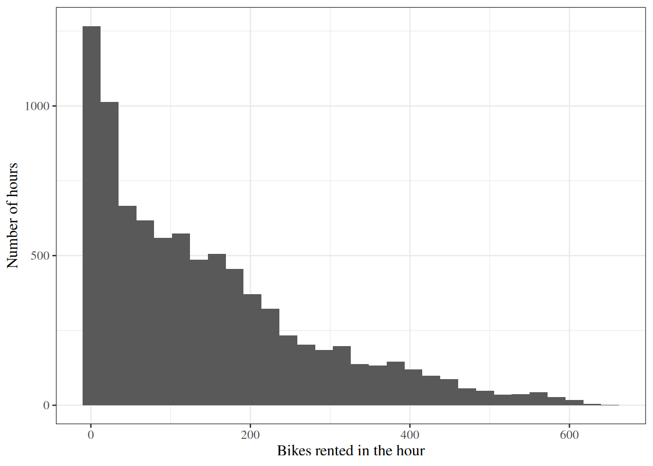
Exercise 3 (A histogram of the hourly count) The Bikeshare data count the bikes rented in each of many hours, as bikers. A histogram shows the shape of the whole set of counts.
Hint
ggplot2::geom_histogram() in R, hist() in R without the tidyverse, and ax.hist() from matplotlib in Python draw a histogram.
Draw a histogram of bikers.
Solution 3.
[Code]
# 30 bars of equal width, from the smallest count to the largest.
bikers_range <- range(bikeshare_raw$bikers)
bikers_breaks <- seq(
  bikers_range[1],
  bikers_range[2],
  length.out = 31 # check-unexplained-choices: allow
)
hist(
  bikeshare_raw$bikers,
  breaks = bikers_breaks, # check-unexplained-choices: allow
  main = NULL,
  xlab = "Bikes rented in the hour",
  ylab = "Number of hours"
)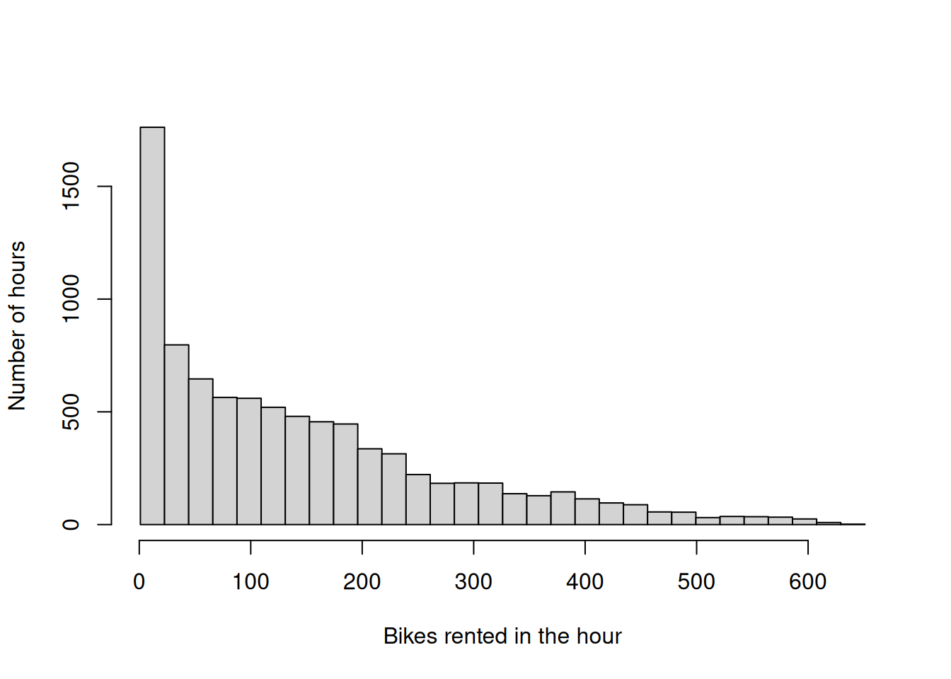
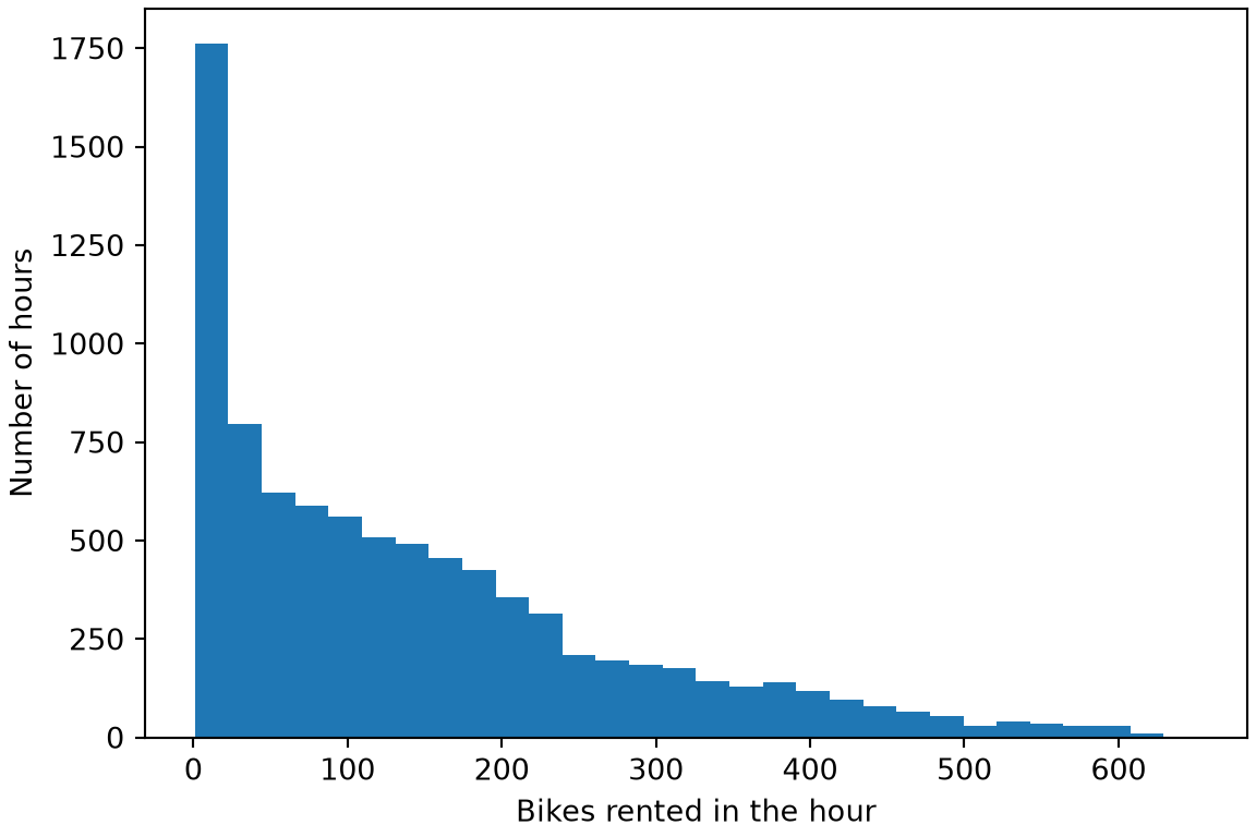
I chose 30 bars, which is about 288 hours per bar. Far fewer bars would hide the long right tail inside a few wide bars, and far more would leave most bars with only a few hours, so the outline would look ragged.
The histogram is right-skewed: the sample median of bikers is 109, below its sample mean of 143.8. Counts cannot be negative, and nothing caps them, which is the situation that a Poisson regression model is built for.
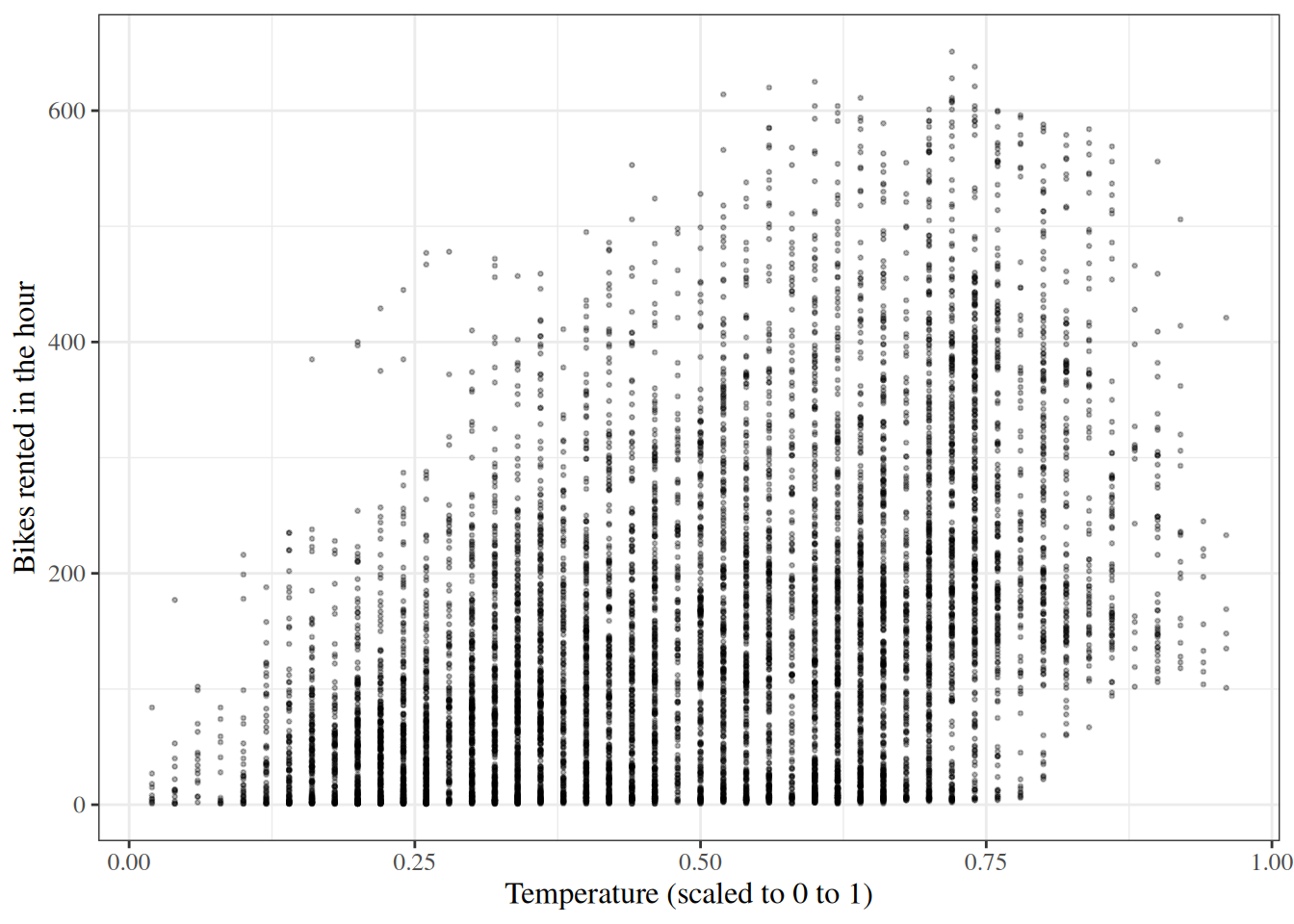
Exercise 4 (Rentals against temperature) The Bikeshare data record the scaled temperature of each hour as temp, and the number of bikes rented in that hour as bikers. A scatterplot shows how the counts change with a numerical covariate.
Hint
ggplot2::geom_point() in R, plot() in R without the tidyverse, and ax.scatter() from matplotlib in Python draw a scatterplot.
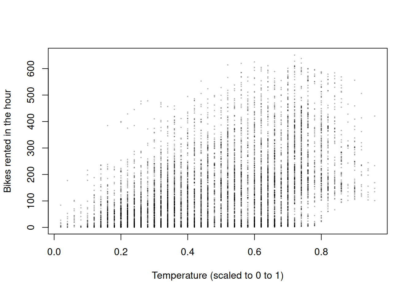
Draw a scatterplot of bikers against temp.
Solution 4.
[Code]
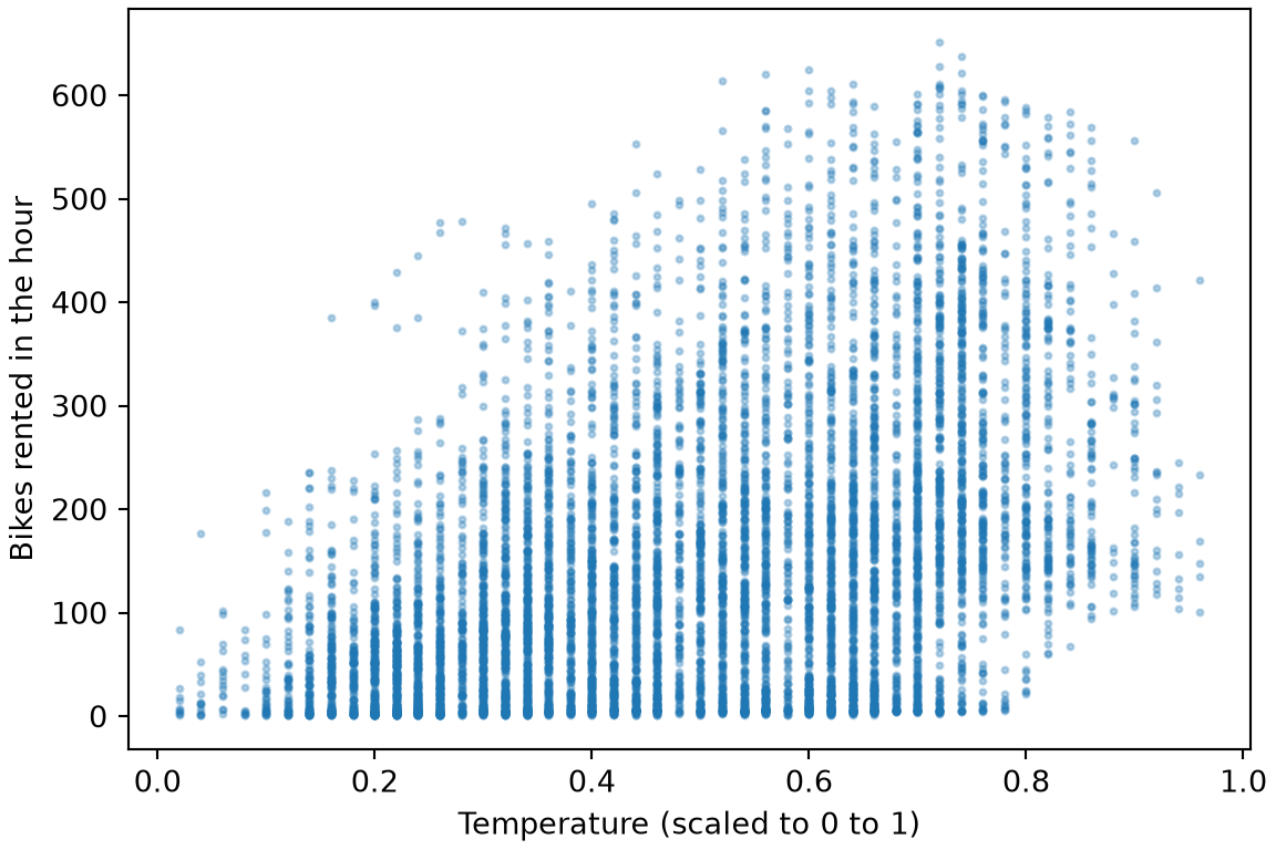
The counts rise with the temperature, with sample correlation 0.45. The spread of the counts grows with their level. A Poisson regression model describes that pattern, because the variance of a Poisson variable is the same as its expected value.
Exercise 5 (Fit a Poisson regression to bike rentals) The Bikeshare data count the bikes rented in each of many hours. Each count covers one hour, so every count has the same exposure magnitude. Consider a Poisson regression model of the hourly count bikers on the covariates temp, workingday, and weathersit, with clear as the reference level of weathersit.
Hint
In R, glm() with family = poisson fits the model. In Python, the statsmodels function smf.glm() fits it with family=sm.families.Poisson(). Both code weathersit as one dummy variable for each level except the reference level.
Solution 5.
[Code]
# Make `clear` the first level of weathersit,
# so that glm() uses it as the reference level.
weather_levels <- c(
  "clear", "cloudy/misty",
  "light rain/snow", "heavy rain/snow"
)
bike <- readr::read_csv("data/bikeshare.csv", show_col_types = FALSE) |>
  dplyr::mutate(weathersit = factor(weathersit, levels = weather_levels))

# Poisson regression of the hourly count on the three covariates.
pois_r <- glm(
  bikers ~ temp + workingday + weathersit,
  family = poisson,
  data = bike
)
pois_coef <- coef(pois_r)
pois_r |>
  parameters::parameters() |>
parameters::print_md()| Parameter | Log-Mean | SE | 95% CI | z | p |
|---|---|---|---|---|---|
| (Intercept) | 3.89 | 3.23e-03 | (3.88, 3.89) | 1202.49 | < .001 |
| temp | 2.13 | 4.79e-03 | (2.12, 2.14) | 444.59 | < .001 |
| workingday | -8.89e-03 | 1.94e-03 | (-0.01, -5.08e-03) | -4.57 | < .001 |
| weathersit (cloudy/misty) | -0.04 | 2.13e-03 | (-0.05, -0.04) | -19.81 | < .001 |
| weathersit (light rain/snow) | -0.43 | 4.02e-03 | (-0.44, -0.42) | -107.41 | < .001 |
| weathersit (heavy rain/snow) | -0.76 | 0.17 | (-1.11, -0.45) | -4.57 | < .001 |
[Code]
# Make `clear` the first level of weathersit,
# so that glm() uses it as the reference level.
weather_levels <- c(
  "clear", "cloudy/misty",
  "light rain/snow", "heavy rain/snow"
)
# nolint next: undesirable_function_linter. This tab shows base R.
bike_base <- read.csv("data/bikeshare.csv")
bike_base$weathersit <- factor(bike_base$weathersit, levels = weather_levels)

# Poisson regression of the hourly count on the three covariates.
pois_base <- glm(
  bikers ~ temp + workingday + weathersit,
  family = poisson,
  data = bike_base
)
pois_base_summary <- summary(pois_base)
round(pois_base_summary$coefficients, 3)
#>                           Estimate Std. Error  z value Pr(>|z|)
#> (Intercept)                  3.885      0.003 1202.490        0
#> temp                         2.129      0.005  444.587        0
#> workingday                  -0.009      0.002   -4.574        0
#> weathersitcloudy/misty      -0.042      0.002  -19.805        0
#> weathersitlight rain/snow   -0.432      0.004 -107.412        0
#> weathersitheavy rain/snow   -0.761      0.167   -4.566        0
[Code]
import pandas as pd
import statsmodels.api as sm
import statsmodels.formula.api as smf

bike = pd.read_csv("data/bikeshare.csv")
# Poisson regression of the hourly count on the three covariates,
# with `clear` as the reference level of weathersit.
pois_py = smf.glm(
    "bikers ~ temp + workingday + C(weathersit, Treatment('clear'))",
    data=bike,
    family=sm.families.Poisson(),
).fit()
pois_py.params.round(3)
#> Intercept                                               3.885
#> C(weathersit, Treatment('clear'))[T.cloudy/misty]      -0.042
#> C(weathersit, Treatment('clear'))[T.heavy rain/snow]   -0.761
#> C(weathersit, Treatment('clear'))[T.light rain/snow]   -0.432
#> temp                                                    2.129
#> workingday                                             -0.009
#> dtype: float64
All three tabs fit the same model with the same reference level, clear, so their coefficient estimates agree. The coefficient estimate of temp is 2.13, a positive number, so the event rate of the fitted model rises with the temperature.
Exercise 6 (Interpret the temperature coefficient) Use the Poisson regression model of Exercise 5. Consider two hours with the same workingday and weathersit, one with temp \(0.1\) higher than the other.
Hint
The Poisson regression model of Exercise 5 has no interactions or transformations involving temp, so Theorem 1 applies.
Estimate the rate ratio comparing the warmer hour with the cooler one.
Solution 6.
By Theorem 1 with \(a - b = 0.1\), the rate ratio is \({\operatorname{exp}\mathopen{}\left\{0.1 \beta_{\text{temp}}\right\}\mathclose{}}\), and its estimate is \({\operatorname{exp}\mathopen{}\left\{0.1 \hat{\beta}_{\text{temp}}\right\}\mathclose{}}\). That estimate is 1.24 in the R tab and 1.24 in the Python tab, so the estimated event rate of the warmer hour is about 1.24 times that of the cooler hour.
Exercise 7 (Compare with linear regression) Consider a linear regression of bikers on the same covariates as the Poisson regression model of Exercise 5. A count is never negative.
Hint
lm() in R and smf.ols() in Python fit the linear regression. fitted() in R returns the fitted values of a model, and the fittedvalues attribute of a statsmodels fit holds them in Python.
For each of the two fitted models, count the hours with a negative fitted value.
Solution 7.
[Code]
# `bike`, `pois_r` and `pois_py` come from the solution to the fit exercise.
# Linear regression on the same covariates as the Poisson model.
lin_r <- lm(bikers ~ temp + workingday + weathersit, data = bike)

# Count the hours whose fitted value is below zero, for each model.
fitted_lin_r <- fitted(lin_r)
fitted_pois_r <- fitted(pois_r)
n_neg_lin_r <- sum(fitted_lin_r < 0)
n_neg_pois_r <- sum(fitted_pois_r < 0)
c(linear = n_neg_lin_r, poisson = n_neg_pois_r)
#>  linear poisson
#>      20       0
[Code]
# `bike`, `pois_r` and `pois_py` come from the solution to the fit exercise.
# Linear regression on the same covariates as the Poisson model.
lin_py = smf.ols(
    "bikers ~ temp + workingday + C(weathersit, Treatment('clear'))",
    data=bike,
).fit()

# Count the hours whose fitted value is below zero, for each model.
n_neg_lin_py = int((lin_py.fittedvalues < 0).sum())
n_neg_pois_py = int((pois_py.fittedvalues < 0).sum())
{"linear": n_neg_lin_py, "poisson": n_neg_pois_py}
#> {'linear': 20, 'poisson': 0}
The linear regression gives a negative fitted value for 20 hours, which is impossible for the expected value of a count.
The Poisson regression model gives a negative fitted value for 0 hours, because its event rate is the exponential function of a linear function, and the exponential function takes only positive values.
[1]
G. James, D. Witten, T. Hastie, and R. Tibshirani, An introduction to statistical learning: With applications in R, 2nd ed. Springer, 2021. doi: 10.1007/978-1-0716-1418-1.