Comparing Means
Last modified: 2026-11-07 21:34:29 (PST)
1 Introduction
This page reviews the standard methods for comparing the mean of a continuous outcome between groups: t-tests, confidence intervals for a difference in means, and one-way analysis of variance.
This page builds on three others:
- Exploratory Data Analysis defines the sample statistics these methods use;
- Statistical Inference defines hypotheses, test statistics, p-values, confidence intervals, and the t, chi-square, and F reference distributions;
- Estimation defines estimators and their standard errors.
The t-tests and ANOVA on this page are the exact, Gaussian-outcome tests in the table of exact and approximate tests on the Maximum Likelihood page, which pairs each one with its large-sample counterpart.
This page is adapted from Vittinghoff et al. [1], Chapter 3.
2 The HERS data
The “heart and estrogen/progestin study” (HERS) was a clinical trial of hormone therapy for prevention of recurrent heart attacks and death among 2,763 post-menopausal women with existing coronary heart disease (CHD) [2].
The trial was conducted at 20 US clinical centers. Participants were randomized to receive either conjugated equine estrogens (0.625 mg/day) plus medroxyprogesterone acetate (2.5 mg/day) or a matching placebo [2]. Women were followed for an average of 4.1 years [2].
The primary outcome was nonfatal myocardial infarction or CHD death [2].
The HERS data are distributed with Vittinghoff et al. [1] on the book’s companion website, as a Stata file that R can read directly:
The rmb R package includes the same file, which these notes use so that rendering does not depend on the website. haven::as_factor() converts the Stata value labels to factors:
The examples on this page use these variables:
| Variable | Meaning |
|---|---|
HT |
Randomized treatment: placebo or hormone therapy |
age |
Age at baseline (years) |
raceth |
Race/ethnicity: White, African American, or Other |
exercise |
Exercises at least three times per week (no/yes) |
BMI |
Body mass index at baseline (kg/m2) |
SBP |
Systolic blood pressure at baseline (mmHg) |
glucose |
Fasting glucose at baseline (mg/dL) |
glucose1 |
Fasting glucose at the year-1 visit (mg/dL) |
hers |>
  dplyr::select(HT, age, raceth, exercise, BMI, SBP, glucose, glucose1) |>
  dplyr::glimpse()
#> Rows: 2,763
#> Columns: 8
#> $ HT       <fct> placebo, placebo, hormone therapy, placebo, placebo, hormone …
#> $ age      <dbl> 70, 62, 69, 64, 65, 68, 70, 69, 61, 62, 72, 73, 52, 57, 57, 6…
#> $ raceth   <fct> African American, African American, White, White, White, Afri…
#> $ exercise <fct> no, no, no, no, no, no, no, yes, yes, no, no, no, no, no, yes…
#> $ BMI      <dbl> 23.69, 28.62, 42.51, 24.39, 21.90, 29.05, 34.45, 23.16, 30.26…
#> $ SBP      <dbl> 138, 118, 134, 152, 175, 174, 119, 178, 162, 111, 122, 158, 1…
#> $ glucose  <dbl> 84, 111, 114, 94, 101, 116, 120, 95, 105, 98, 111, 95, 97, 10…
#> $ glucose1 <dbl> 94, 78, 98, 93, 92, 115, NA, 95, 113, 98, 96, 107, 90, 100, 1…
3 Descriptive statistics
The Exploratory Data Analysis page defines the sample statistics used on this page, each with an example:
- the sample mean;
- the sample median;
- the sample variance;
- the sample standard deviation;
- the interquartile range;
- the sample proportion.
That page also defines the graphs used here, including box plots and scatter plots.
Example 1 (HERS baseline characteristics by treatment group) Table 1 summarizes the HERS participants at baseline, separately for each randomized group. Continuous variables are summarized by sample mean (standard deviation), and categorical variables by count (percent).
[Code]
hers |>
  dplyr::select(
    age, BMI, glucose, SBP, DBP,
    HT, raceth, exercise, smoking, diabetes
  ) |>
  gtsummary::tbl_summary(
    by = HT,
    statistic = list(
      gtsummary::all_continuous() ~ "{mean} ({sd})",
      gtsummary::all_categorical() ~ "{n} ({p}%)"
    ),
    digits = gtsummary::all_continuous() ~ 1,
    label = list(
      age ~ "Age (years)",
      BMI ~ "BMI (kg/m^2)",
      glucose ~ "Fasting glucose (mg/dL)",
      SBP ~ "Systolic BP (mmHg)",
      DBP ~ "Diastolic BP (mmHg)",
      raceth ~ "Race/ethnicity",
      exercise ~ "Exercises regularly",
      smoking ~ "Current smoker",
      diabetes ~ "Diabetes"
    )
  ) |>
  gtsummary::add_overall() |>
gtsummary::bold_labels()| Characteristic |
Overall N = 2,7631 |
placebo N = 1,3831 |
hormone therapy N = 1,3801 |
|---|---|---|---|
| Age (years) | 66.6 (6.7) | 66.8 (6.7) | 66.5 (6.6) |
| BMI (kg/m^2) | 28.6 (5.5) | 28.5 (5.5) | 28.6 (5.5) |
| Unknown | 5 | 4 | 1 |
| Fasting glucose (mg/dL) | 112.2 (36.8) | 112.4 (36.8) | 111.9 (36.9) |
| Systolic BP (mmHg) | 135.1 (19.0) | 135.1 (19.4) | 135.0 (18.7) |
| Diastolic BP (mmHg) | 73.2 (9.7) | 73.1 (9.7) | 73.2 (9.7) |
| Unknown | 1 | 1 | 0 |
| Race/ethnicity | |||
| White | 2,451 (89%) | 1,239 (90%) | 1,212 (88%) |
| African American | 218 (7.9%) | 102 (7.4%) | 116 (8.4%) |
| Other | 94 (3.4%) | 42 (3.0%) | 52 (3.8%) |
| Exercises regularly | 1,068 (39%) | 530 (38%) | 538 (39%) |
| Current smoker | 360 (13%) | 182 (13%) | 178 (13%) |
| Diabetes | 731 (26%) | 352 (25%) | 379 (27%) |
| 1 Mean (SD); n (%) | |||
Because treatment was assigned at random, the two groups differ at baseline only by chance, and their summaries are close.
4 Comparing two groups: continuous outcomes
4.1 Hypotheses
The Statistical Inference page defines the null hypothesis, the alternative hypothesis, test statistics, p-values, and significance levels. In a comparison of two groups with means \(\mu_1\) and \(\mu_2\), the null hypothesis is usually \(H_0: \mu_1 = \mu_2\), and the two-sided alternative is \(H_1: \mu_1 \neq \mu_2\).
4.2 One-sample t-test
Definition 1 (One-sample t-test) Let \(x_1, \ldots, x_n\) be observations with \(n \ge 2\), sample mean \({\bar{x}}\), and sample standard deviation \(s\). The one-sample t-test of \(H_0: \mu= \mu_0\) against \(H_1: \mu\neq \mu_0\) uses the statistic
\[t \stackrel{\text{def}}{=}\frac{{\bar{x}}- \mu_0}{s / \sqrt{n}}.\]
Its p-value is \(\Pr(\mathopen{}\left|T\right|\mathclose{} \ge \mathopen{}\left|t\right|\mathclose{})\), where \(T\) has the \(t_{n-1}\) distribution (t-distribution).
Source: Wikipedia contributors [3].
Theorem 1 (Null distribution of the one-sample t statistic) Let \(X_1, \ldots, X_n\) be independent, each Gaussian with mean \(\mu_0\) and variance \(\sigma^2\), with \(n \ge 2\). Then the statistic \(T \stackrel{\text{def}}{=}(\bar X - \mu_0) / (S / \sqrt{n})\) of Definition 1, computed from these random variables, has the \(t_{n-1}\) distribution.
Proof. We use a standard fact about Gaussian samples [4, Sec. 5.5], pp. 203-205: \(\bar X\) and \(S^2\) are independent, and \(V \stackrel{\text{def}}{=}(n-1) S^2 / \sigma^2\) has the \(\chi^2_{n-1}\) distribution. Also, \(Z \stackrel{\text{def}}{=}(\bar X - \mu_0) / (\sigma/ \sqrt{n})\) has the standard Gaussian distribution, and \(Z\) is independent of \(V\) because \(\bar X\) is independent of \(S^2\). So by the definition of the t-distribution, \(Z / \sqrt{V / (n-1)}\) has the \(t_{n-1}\) distribution, and this ratio equals \(T\):
\[ \begin{aligned} \frac{Z}{\sqrt{V/(n-1)}} &= \frac{(\bar X - \mu_0) / (\sigma/ \sqrt{n})}{\sqrt{S^2 / \sigma^2}} && \text{(substitute $Z$ and $V$)}\\ &= \frac{(\bar X - \mu_0) / (\sigma/ \sqrt{n})}{S / \sigma} && \text{($\sqrt{S^2} = S$, since $S \ge 0$)}\\ &= \frac{\bar X - \mu_0}{S / \sqrt{n}} && \text{(the factors of $\sigma$ cancel)}\\ &= T. \end{aligned} \]
Remark 1 (Non-Gaussian data). When the observations are not Gaussian, \(T\) still has approximately the standard Gaussian distribution when \(n\) is large, by the central limit theorem, and then \(t_{n-1}\) is close to the standard Gaussian distribution (t quantiles approach Gaussian quantiles).
4.3 Paired t-test
Definition 2 (Paired t-test) Let \((x_{1,1}, x_{1,2}), \ldots, (x_{n,1}, x_{n,2})\) be pairs of related measurements, such as the same participants measured at two times, and let \(d_i \stackrel{\text{def}}{=}x_{i,2} - x_{i,1}\) be the within-pair differences, with population mean \(\mu_d\). The paired t-test of \(H_0: \mu_d = 0\) against \(H_1: \mu_d \neq 0\) is the one-sample t-test (Definition 1) of \(H_0: \mu= 0\) applied to \(d_1, \ldots, d_n\).
Source: Wikipedia contributors [3].
Example 2 (Change in fasting glucose over the first year of HERS) We test whether mean fasting glucose changed between baseline (glucose) and the year-1 visit (glucose1), across both treatment groups. Participants missing either measurement are dropped. The t statistic of Definition 1, computed on the differences:
glucose_change <- hers |>
  dplyr::filter(!is.na(glucose), !is.na(glucose1)) |>
  dplyr::mutate(d = glucose1 - glucose) |>
  dplyr::pull(d)
n_pairs <- length(glucose_change)
t_paired <- mean(glucose_change) / (sd(glucose_change) / sqrt(n_pairs))
c(
  n = n_pairs,
  mean_change = mean(glucose_change),
  t = t_paired,
  p_value = 2 * pt(-abs(t_paired), df = n_pairs - 1)
)
#>           n mean_change           t     p_value
#> 2.61300e+03 2.62036e+00 4.15081e+00 3.41911e-05
t.test() with paired = TRUE gives the same statistic, along with a confidence interval for \(\mu_d\):
t.test(hers$glucose1, hers$glucose, paired = TRUE)
#>
#>  Paired t-test
#>
#> data:  hers$glucose1 and hers$glucose
#> t = 4.151, df = 2612, p-value = 3.42e-05
#> alternative hypothesis: true mean difference is not equal to 0
#> 95 percent confidence interval:
#>  1.38248 3.85824
#> sample estimates:
#> mean difference
#>         2.62036
Mean fasting glucose rose by about 2.6 mg/dL over the year, and the p-value is far below 0.05.
4.4 Two-sample t-tests
Definition 3 (Welch’s two-sample t-test) Let two independent groups have sample sizes \(n_1, n_2 \ge 2\), sample means \(\bar{x}_1\) and \(\bar{x}_2\), and sample variances \(s_1^2\) and \(s_2^2\). Welch’s two-sample t-test of \(H_0: \mu_1 = \mu_2\) against \(H_1: \mu_1 \neq \mu_2\) uses the statistic
\[t \stackrel{\text{def}}{=}\frac{\bar{x}_1 - \bar{x}_2}{\sqrt{\dfrac{s_1^2}{n_1} + \dfrac{s_2^2}{n_2}}}\]
and the Welch–Satterthwaite degrees of freedom
\[\hat{\operatorname{df}}\stackrel{\text{def}}{=}\frac{\mathopen{}\left(\dfrac{s_1^2}{n_1} + \dfrac{s_2^2}{n_2}\right)\mathclose{}^2} {\dfrac{(s_1^2 / n_1)^2}{n_1 - 1} + \dfrac{(s_2^2 / n_2)^2}{n_2 - 1}}.\]
Its p-value is \(\Pr(\mathopen{}\left|T\right|\mathclose{} \ge \mathopen{}\left|t\right|\mathclose{})\), where \(T\) has the \(t_{\hat{\operatorname{df}}}\) distribution (t-distribution).
Source: Wikipedia contributors [5].
Remark 2 (Properties of Welch’s test). Welch’s test does not assume that the two groups have equal variances. Even for Gaussian data, \(t_{\hat{\operatorname{df}}}\) is only an approximation to the null distribution of \(t\). For large groups, the central limit theorem makes the statistic approximately standard Gaussian under \(H_0\), as in the WCGS cholesterol example. Welch’s test is the default in R’s t.test().
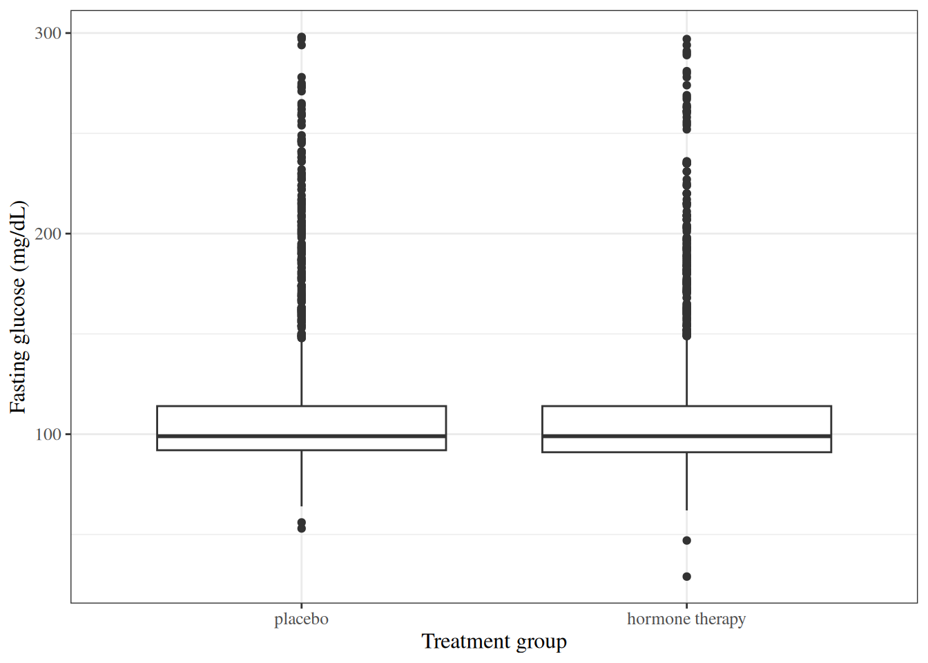
Example 3 (Baseline fasting glucose by treatment group in HERS) We test \(H_0: \mu_\text{HT} = \mu_\text{placebo}\) against \(H_1: \mu_\text{HT} \neq \mu_\text{placebo}\), where \(\mu_\text{HT}\) and \(\mu_\text{placebo}\) are the population mean baseline fasting glucose levels in the hormone therapy and placebo populations. Figure 1 compares the two groups’ distributions.
[Code]
The statistic and degrees of freedom of Definition 3:
glucose_ht <- hers |>
  dplyr::filter(HT == "hormone therapy") |>
  dplyr::pull(glucose)
glucose_placebo <- hers |>
  dplyr::filter(HT == "placebo") |>
  dplyr::pull(glucose)
v_ht <- var(glucose_ht) / length(glucose_ht)
v_placebo <- var(glucose_placebo) / length(glucose_placebo)
t_welch <- (mean(glucose_ht) - mean(glucose_placebo)) / sqrt(v_ht + v_placebo)
df_welch <- (v_ht + v_placebo)^2 /
  (v_ht^2 / (length(glucose_ht) - 1) +
     v_placebo^2 / (length(glucose_placebo) - 1))
c(t = t_welch, df = df_welch, p_value = 2 * pt(-abs(t_welch), df_welch))
#>           t          df     p_value
#>   -0.424594 2760.978546    0.671165
t.test() reports the same values:
t.test(glucose_ht, glucose_placebo)
#>
#>  Welch Two Sample t-test
#>
#> data:  glucose_ht and glucose_placebo
#> t = -0.4246, df = 2761, p-value = 0.671
#> alternative hypothesis: true difference in means is not equal to 0
#> 95 percent confidence interval:
#>  -3.34503  2.15423
#> sample estimates:
#> mean of x mean of y
#>   111.854   112.449
The p-value is large, so the data give no evidence against \(H_0\). That result is expected here: treatment was randomized, so the groups’ baseline sample means differ only by chance.
Definition 4 (Pooled variance) For two samples of sizes \(n_1\) and \(n_2\) with sample variances \(s_1^2\) and \(s_2^2\), the pooled variance is
\[s_p^2 \stackrel{\text{def}}{=}\frac{(n_1 - 1) s_1^2 + (n_2 - 1) s_2^2}{n_1 + n_2 - 2}.\]
Source: Wikipedia contributors [6].
Example 4 (Pooled variance of two small samples) With \(n_1 = 3\), \(s_1^2 = 4\), \(n_2 = 5\), and \(s_2^2 = 9\):
\[ \begin{aligned} s_p^2 &= \frac{(3 - 1) \cdot 4 + (5 - 1) \cdot 9}{3 + 5 - 2} && \text{(definition of pooled variance)}\\ &= \frac{8 + 36}{6} && \text{(arithmetic)}\\ &\approx 7.33 && \text{(arithmetic)} \end{aligned} \]
The pooled variance lies between the two sample variances, closer to \(s_2^2\), whose sample is larger.
Remark 3 (What the pooled variance estimates). When the two populations share one variance \(\sigma^2\), the pooled variance estimates it.
Definition 5 (Pooled two-sample t-test) With the notation of Definition 3 and the pooled variance \(s_p^2\), the pooled two-sample t-test of \(H_0: \mu_1 = \mu_2\) uses the statistic
\[t_p \stackrel{\text{def}}{=}\frac{\bar{x}_1 - \bar{x}_2}{s_p \sqrt{\dfrac{1}{n_1} + \dfrac{1}{n_2}}}.\]
Its p-value is \(\Pr(\mathopen{}\left|T\right|\mathclose{} \ge \mathopen{}\left|t_p\right|\mathclose{})\), where \(T\) has the \(t_{n_1 + n_2 - 2}\) distribution.
Source: Wikipedia contributors [3].
Theorem 2 (Null distribution of the pooled t statistic) Let the observations in both groups be independent and Gaussian, all with the same mean and the same variance \(\sigma^2\). Then \(t_p\) (Definition 5), computed from these random variables, has the \(t_{n_1 + n_2 - 2}\) distribution [4, Sec. 8.2], p. 371.
Remark 4 (The equal-variance assumption). Theorem 2 needs equal variances in the two groups, and Welch’s test (Definition 3) does not, so these notes use Welch’s test by default.
Example 5 (Pooled t-test of baseline glucose in HERS) In HERS, the two groups have nearly equal sizes (1380 and 1383) and nearly equal standard deviations (36.9 and 36.8 mg/dL), so the pooled test gives almost the same result as Welch’s test in Example 3:
t.test(glucose_ht, glucose_placebo, var.equal = TRUE)
#>
#>  Two Sample t-test
#>
#> data:  glucose_ht and glucose_placebo
#> t = -0.4246, df = 2761, p-value = 0.671
#> alternative hypothesis: true difference in means is not equal to 0
#> 95 percent confidence interval:
#>  -3.34502  2.15422
#> sample estimates:
#> mean of x mean of y
#> 111.854 112.449- Hogg et al. [4, Sec. 8.2], pp. 369–377 covers tests of the equality of two means.
- Rice [7, Sec. 11.2.1], pp. 421–432 covers normal-theory methods for two independent samples.
- Rice [7, Sec. 11.3.1], pp. 446–447 covers normal-theory methods for paired samples.
4.5 Confidence intervals for the difference in means
Definition 6 (Welch confidence interval for a difference in means) With the notation of Definition 3, the Welch \(100(1-\alpha)\%\) confidence interval for \(\mu_1 - \mu_2\) is
\[(\bar{x}_1 - \bar{x}_2) \pm t_{\hat{\operatorname{df}},\, 1 - \alpha/2} \sqrt{\frac{s_1^2}{n_1} + \frac{s_2^2}{n_2}},\]
where \(t_{\hat{\operatorname{df}},\, 1 - \alpha/2}\) is the \(1 - \alpha/2\) quantile of the \(t_{\hat{\operatorname{df}}}\) distribution. It is an approximate confidence interval.
Example 6 (Confidence interval for the HERS baseline glucose difference) Continuing Example 3, the 95% interval of Definition 6 is:
This interval matches the one t.test() reports in Example 3. It contains 0, consistent with the large p-value there.
Hogg et al. [4, Sec. 7.2], pp. 314–322 covers confidence intervals for the difference of two means.
5 One-way analysis of variance
Definition 7 (Between-group sum of squares) Let \(y_{j1}, \ldots, y_{jn_j}\) be the \(n_j\) observations in group \(j\), for \(k \ge 2\) groups with \(n \stackrel{\text{def}}{=}\sum_{j=1}^{k} n_j\) observations in all, let \({\bar{y}}_j\) be the sample mean of group \(j\), and let \({\bar{y}}\) be the sample mean of all \(n\) observations. The between-group sum of squares is
\[\text{SS}_\text{between} \stackrel{\text{def}}{=}\sum_{j=1}^{k} n_j ({\bar{y}}_j - {\bar{y}})^2.\]
Source: Wikipedia contributors [8].
Example 7 (Between-group sum of squares of two small groups) Let group 1 be \(\mathopen{}\left\{1, 2, 3\right\}\mathclose{}\) and group 2 be \(\mathopen{}\left\{4, 5, 6\right\}\mathclose{}\), so \(\bar y_1 = 2\), \(\bar y_2 = 5\), and \(\bar y = 3.5\). Then:
\[ \begin{aligned} \text{SS}_\text{between} &= 3(2 - 3.5)^2 + 3(5 - 3.5)^2 && \text{(definition)}\\ &= 3(2.25) + 3(2.25) && \text{(square the deviations)}\\ &= 13.5 && \text{(arithmetic)} \end{aligned} \]
Definition 8 (Within-group sum of squares) With the notation of Definition 7, the within-group sum of squares is
\[\text{SS}_\text{within} \stackrel{\text{def}}{=}\sum_{j=1}^{k} \sum_{i=1}^{n_j} (y_{ji} - {\bar{y}}_j)^2.\]
Source: Wikipedia contributors [8].
Example 8 (Within-group sum of squares of two small groups) For the groups of Example 7:
\[ \begin{aligned} \text{SS}_\text{within} &= \mathopen{}\left[(1-2)^2 + (2-2)^2 + (3-2)^2\right]\mathclose{} + \mathopen{}\left[(4-5)^2 + (5-5)^2 + (6-5)^2\right]\mathclose{} && \text{(definition)}\\ &= 2 + 2 && \text{(arithmetic)}\\ &= 4 && \text{(arithmetic)} \end{aligned} \]
Definition 9 (Mean squares) In one-way analysis of variance, the mean squares are the sums of squares divided by their degrees of freedom: \(\text{MS}_\text{between} \stackrel{\text{def}}{=}\text{SS}_\text{between} / (k - 1)\) and \(\text{MS}_\text{within} \stackrel{\text{def}}{=}\text{SS}_\text{within} / (n - k)\). When the \(k\) groups share one variance \(\sigma^2\), \(\text{MS}_\text{within}\) estimates it.
Example 9 (Mean squares of two small groups) For the groups of Example 7, \(k = 2\) and \(n = 6\), so
\[ \begin{aligned} \text{MS}_\text{between} &= 13.5 / 1 \\ &= 13.5 \end{aligned} \]
and
\[ \begin{aligned} \text{MS}_\text{within} &= 4 / 4 \\ &= 1. \end{aligned} \]
Definition 10 (One-way analysis of variance) With the mean squares of \(k \ge 2\) groups and \(n > k\) observations in all, the one-way analysis of variance (ANOVA) F-test of
\[ \begin{aligned} H_0: \mu_1 &= \mu_2 \\ &= \cdots \\ &= \mu_k \end{aligned} \]
against the alternative that at least two group means differ uses the statistic [9]
\[F \stackrel{\text{def}}{=}\frac{\text{MS}_\text{between}}{\text{MS}_\text{within}}.\]
Its p-value is \(\Pr(F^* \ge F)\), where \(F^*\) has the \(F_{k-1,\, n-k}\) distribution (F-distribution).
Source: Wikipedia contributors [10].
Remark 5 (Interpreting the F statistic). Large values of \(F\) mean that the group means are spread out more than the variation within groups would explain. For the groups of Example 9,
\[ \begin{aligned} F &= 13.5 / 1 \\ &= 13.5. \end{aligned} \]
Theorem 3 (Null distribution of the ANOVA F statistic) Let all \(n\) observations be independent, with observation \(y_{ji}\) Gaussian with mean \(\mu_j\) and the same variance \(\sigma^2\) in every group. If
\[ \begin{aligned} H_0: \mu_1 &= \cdots \\ &= \mu_k \end{aligned} \]
holds, then \(F\) (Definition 10), computed from these random variables, has the \(F_{k-1,\, n-k}\) distribution [4, Sec. 9.3], p. 449.
Example 10 (Fasting glucose by race/ethnicity in HERS) The group sizes, sample means, and sample standard deviations of baseline fasting glucose:
The F statistic of Definition 10, computed step by step:
anova_parts <- hers |>
  dplyr::mutate(grand_mean = mean(glucose)) |>
  dplyr::mutate(.by = raceth, group_mean = mean(glucose)) |>
  dplyr::summarize(
    ss_between = sum((group_mean - grand_mean)^2),
    ss_within = sum((glucose - group_mean)^2),
    k = dplyr::n_distinct(raceth),
    n = dplyr::n()
  ) |>
  dplyr::mutate(
    f = (ss_between / (k - 1)) / (ss_within / (n - k)),
    p_value = pf(f, k - 1, n - k, lower.tail = FALSE)
  )
anova_parts
\(\text{SS}_\text{between}\) is summed here over observations rather than groups: each observation in group \(j\) contributes \(({\bar{y}}_j - {\bar{y}})^2\), which gives the \(n_j\) weights of Definition 10. aov() reports the same sums of squares, F statistic, and p-value:
| Parameter | Sum_Squares | df | Mean_Square | F | p |
|---|---|---|---|---|---|
| raceth | 45918.814 | 2 | 22959.407 | 17.105 | < .001 |
| Residuals | 3.705e+06 | 2760 | 1342.226 |
Anova Table (Type 1 tests)
The p-value is far below 0.05: population mean fasting glucose differs among the three race/ethnicity groups.
Remark 6 (Unequal variances in the HERS glucose groups). The group standard deviations differ, from 36 to 44 mg/dL, so the equal-variance condition of Theorem 3 is questionable. oneway.test() performs Welch’s version of the F-test, which does not assume equal variances, and reaches the same conclusion:
One-way ANOVA is a special case of linear regression: it is the F-test comparing a linear regression model with a single categorical predictor to the model with an intercept only (Linear Models Overview). lm() gives the same F statistic as aov():
| Parameter | Sum_Squares | df | Mean_Square | F | p |
|---|---|---|---|---|---|
| raceth | 45918.814 | 2 | 22959.407 | 17.105 | < .001 |
| Residuals | 3.705e+06 | 2760 | 1342.226 |
With \(k = 2\) groups, the ANOVA F statistic equals the square of the pooled t statistic (Definition 5), as the two treatment groups of Example 5 show:
- Hogg et al. [4, Sec. 9.3], pp. 446–455 covers one-factor analysis of variance.
- Casella and Berger [11, Sec. 11.2], pp. 522–538 covers oneway analysis of variance.
- Rice [7, Sec. 12.2], pp. 477–488 covers the one-way layout.