Permutation Tests
Last modified: 2026-10-27 23:24:14 (PDT)
The p-value of a t-test comes from a distributional approximation: the statistic is only approximately t-distributed unless the data are Gaussian. A permutation test takes its null distribution from the data instead [1]. If the null hypothesis says that two groups have the same distribution, then under that hypothesis the group labels carry no information, so reassigning the labels at random produces data sets that are as plausible as the observed one. The spread of the test statistic across those relabelings is its null distribution.
This page defines exchangeability, the permutation distribution and the permutation p-value, shows why that p-value is valid, and then approximates it by random relabelings, which is how it is computed in practice. It continues the bootstrap page’s idea of computing a sampling distribution by resampling, and supplies the p-values that the multiple testing page corrects. These notes follow chapter 13 of James et al. [2] and the treatment in Good [3].
1 The Khan gene expression data
The examples on this page use gene expression data from Khan et al. [4], who measured 2308 genes in tissue samples from children with small round blue cell tumors. The samples fall into four tumor classes, numbered 1 to 4 in the data. This site keeps a copy of the 63 training samples at data/khan.csv, taken from the Khan data of the R package ISLR2 [2]: the column tumor_class holds the class, and the columns gene_1 to gene_2308 hold the expression values. The examples compare classes 2 and 4.
2 Exchangeability under the null hypothesis
Definition 1 (Exchangeable random variables) For a permutation \(\pi\) of \({\mathopen{}\left\{1, \ldots, n\right\}\mathclose{}}\) and a vector \(y = (y_1, \ldots, y_n)\), write \(y_\pi \stackrel{\text{def}}{=}(y_{\pi(1)}, \ldots, y_{\pi(n)})\) for the vector with its entries reordered by \(\pi\). Random variables \(Y_1, \ldots, Y_n\) are exchangeable if reordering them does not change their joint distribution: for every permutation \(\pi\) and every set \(A\) of vectors,
\[\Pr(Y_\pi \in A) = \Pr(Y \in A).\]
Source: Wikipedia contributors [5].
Example 1 (Two groups with the same distribution) Let a gene’s expression be measured in \(n_1\) samples from tumor class 2 and \(n_2\) samples from tumor class 4, and let \(H_0\) say that the expression has the same distribution in both classes. Under \(H_0\) the \(n = n_1 + n_2\) values \(Y_1, \ldots, Y_n\) are independent and identically distributed, and independent, identically distributed variables are exchangeable, because their joint distribution is the product of the same marginal distribution \(n\) times, which does not depend on the order of the factors. Given the set of observed values, every assignment of them to the two groups is then equally likely. With 23 samples in class 2 and 20 in class 4 there are
ways to choose which 20 of the 43 values form the class 4 group.
3 The permutation distribution and p-value
3.1 The permutation distribution
Definition 2 (Permutation distribution) Let \(y = (y_1, \ldots, y_n)\) hold the observed values, with the first \(n_1\) entries belonging to group 1 and the rest to group 2, and let \(T(y)\) be a test statistic computed from the data and the group assignment. Let \(S_n\) be the set of all \(n!\) permutations of \({\mathopen{}\left\{1, \ldots, n\right\}\mathclose{}}\). The permutation distribution of \(T\) is the distribution of \(T(y_\pi)\) when \(\pi\) is drawn uniformly from \(S_n\) and \(y\) is held fixed. It puts probability \(1 / n!\) on each relabeling \(y_\pi\), so for every \(t\)
\[\Pr_\pi\mathopen{}\left(T(y_\pi) \ge t\right)\mathclose{} \stackrel{\text{def}}{=}\frac{1}{n!} \sum_{\pi \in S_n} \mathbb{1}_{T(y_\pi) \ge t}.\]
Example 2 (The permutation distribution of six expression values) Take gene 3 in the Khan data, and keep the first three samples from tumor class 2 and the first three from class 4. The test statistic is the absolute value of Welch’s t statistic. Only \(\binom{6}{3} =\) 20 relabelings differ in which values form group 1 (the other \(3! \times 3!\) permutations within each group give the same statistic), so all of them can be listed:
toy <- rbind(
  head(khan_pair[khan_pair$tumor_class == 2, ], 3),
  head(khan_pair[khan_pair$tumor_class == 4, ], 3)
)
y_toy <- toy$gene_3
abs_welch_t <- function(y, in_group1) {
  x1 <- y[in_group1]
  x2 <- y[!in_group1]
  abs(mean(x1) - mean(x2)) / sqrt(var(x1) / length(x1) + var(x2) / length(x2))
}
group1_choices <- combn(6, 3)
t_toy <- apply(
  group1_choices, 2,
  function(idx) abs_welch_t(y_toy, seq_along(y_toy) %in% idx)
)
t_observed_toy <- abs_welch_t(y_toy, seq_along(y_toy) %in% 1:3)
data.frame(
  group_1 = apply(group1_choices, 2, paste, collapse = " "),
  statistic = t_toy
) |>
  dplyr::arrange(dplyr::desc(statistic)) |>
knitr::kable(digits = 3)| group_1 | statistic |
|---|---|
| 1 4 5 | 1.793 |
| 2 3 6 | 1.793 |
| 1 3 5 | 1.624 |
| 2 4 6 | 1.624 |
| 1 2 6 | 1.312 |
| 3 4 5 | 1.312 |
| 1 5 6 | 1.270 |
| 2 3 4 | 1.270 |
| 1 2 3 | 1.019 |
| 4 5 6 | 1.019 |
| 1 2 4 | 0.917 |
| 3 5 6 | 0.917 |
| 1 2 5 | 0.646 |
| 3 4 6 | 0.646 |
| 1 3 6 | 0.463 |
| 2 4 5 | 0.463 |
| 1 4 6 | 0.383 |
| 2 3 5 | 0.383 |
| 1 3 4 | 0.188 |
| 2 5 6 | 0.188 |
The statistics come in equal pairs, because swapping the two groups gives the same absolute value. The observed statistic is 1.019, the value of the relabeling 1 2 3.
3.2 The permutation p-value
Definition 3 (Permutation p-value) With the notation of Definition 2, the permutation p-value of the observed statistic \(t = T(y)\) is the proportion of relabelings whose statistic is at least as extreme as the observed one:
\[p_{\text{perm}} \stackrel{\text{def}}{=}\Pr_\pi\mathopen{}\left(T(y_\pi) \ge T(y)\right)\mathclose{} = \frac{1}{n!} \sum_{\pi \in S_n} \mathbb{1}_{T(y_\pi) \ge T(y)}.\]
Because the identity permutation is one of the \(n!\) relabelings, \(p_{\text{perm}} \ge 1 / n!\).
Source: Wikipedia contributors [6].
Example 3 (Exact permutation p-value for six expression values) Of the 20 relabelings in Example 2, count those whose statistic is at least the observed one. Rounding before the comparison keeps floating-point error from separating values that are equal in exact arithmetic, such as the observed statistic and the one for its mirror image:
The exact permutation p-value is 0.5. With three samples per group the smallest p-value any data could give is \(2 / 20 =\) 0.1, because each statistic has a mirror image, so six samples cannot provide evidence at the 5% level.
Remark 1 (What a permutation test tests). Relabeling is justified only if the null hypothesis makes the labels irrelevant, that is, if the two groups have the same distribution. A permutation test of a difference in means therefore tests the hypothesis of equal distributions. Such a test can reject because the groups differ in spread rather than in mean, and a test that does not assume equal distributions needs a different method.
3.3 Why the permutation p-value is valid
Exercise 1 (Counting values with few larger-or-equal values) Let \(t_1, \ldots, t_N\) be real numbers, and for each \(j\) let \(N_j\) be the number of \(i\) with \(t_i \ge t_j\) (including \(i = j\)). Show that for every integer \(k \ge 0\), at most \(k\) of the \(N_j\) are at most \(k\):
\[\sum_{j=1}^N \mathbb{1}_{N_j \le k} \le k.\]
Solution 1. List the values in decreasing order, breaking ties arbitrarily, so that \(t_{[1]} \ge t_{[2]} \ge \cdots \ge t_{[N]}\). Suppose the value \(t_{[r]}\) at position \(r > k\) has \(N_j \le k\), where \(j\) is its original index. Then the \(r\) values at positions \(1, \ldots, r\) are all at least \(t_{[r]}\), so \(N_j \ge r > k\), which contradicts \(N_j \le k\). So every \(j\) with \(N_j \le k\) sits at a position \(r \le k\) of the sorted list. That list has \(k\) such positions, and each belongs to one index, so at most \(k\) indices have \(N_j \le k\).
Lemma 1 (At most \(k\) values have \(k\) or fewer values at least as large) Let \(t_1, \ldots, t_N\) be real numbers, and for each \(j\) let \(N_j\) be the number of indices \(i\) with \(t_i \ge t_j\) (including \(i = j\)). Then for every integer \(k \ge 0\), at most \(k\) of the \(N_j\) are at most \(k\):
\[\sum_{j=1}^N \mathbb{1}_{N_j \le k} \le k,\]
where \(\mathbb{1}_{A}\) is \(1\) if \(A\) is true and \(0\) otherwise.
Proof. This is the solution to Exercise 1, worked in Solution 1.
Exercise 2 (Relabeling the data permutes the relabelings) For a permutation \(\sigma\) define \(N_\sigma(y)\), the number of relabelings at least as extreme as \(y_\sigma\):
\[N_\sigma(y) \stackrel{\text{def}}{=}\sum_{\pi \in S_n} \mathbb{1}_{T(y_\pi) \ge T(y_\sigma)}.\]
Write \(\iota\) for the identity permutation, so \(N_\iota(y)\) is \(n!\) times the permutation p-value of Definition 3. Express \(N_\sigma(y)\) in terms of \(N_\iota\).
Solution 2. The entries of \((y_\sigma)_{\pi'}\) are \(y_{\sigma(\pi'(i))}\), so \((y_\sigma)_{\pi'} = y_{\sigma \circ \pi'}\).
\[ \begin{aligned} N_\iota(y_\sigma) &= \sum_{\pi' \in S_n} \mathbb{1}_{T\mathopen{}\left((y_\sigma)_{\pi'}\right)\mathclose{} \ge T(y_\sigma)} && \text{(definition, with $y_\sigma$ in place of $y$)}\\ &= \sum_{\pi' \in S_n} \mathbb{1}_{T\mathopen{}\left(y_{\sigma \circ \pi'}\right)\mathclose{} \ge T(y_\sigma)} && \text{($(y_\sigma)_{\pi'} = y_{\sigma \circ \pi'}$)}\\ &= \sum_{\pi \in S_n} \mathbb{1}_{T(y_\pi) \ge T(y_\sigma)} && \text{($\pi = \sigma \circ \pi'$ is a bijection of $S_n$)}\\ &= N_\sigma(y) && \text{(definition)} \end{aligned} \]
So \(N_\sigma(y) = N_\iota(y_\sigma)\).
Lemma 2 (Relabeling the data permutes the relabelings) Let \(T\) be a statistic, let \(y = (y_1, \ldots, y_n)\) be data, let \(S_n\) be the set of permutations of \(\{1, \ldots, n\}\), and let \(y_\sigma\) be \(y\) with its entries relabeled by \(\sigma \in S_n\). For \(\sigma \in S_n\) let \(N_\sigma(y) \stackrel{\text{def}}{=}\sum_{\pi \in S_n} \mathbb{1}_{T(y_\pi) \ge T(y_\sigma)}\) be the number of relabelings at least as extreme as \(y_\sigma\), and write \(\iota\) for the identity permutation, so that \(N_\iota(y)\) is \(n!\) times the permutation p-value of \(T(y)\). Then relabeling the data by \(\sigma\) turns \(N_\iota\) into \(N_\sigma\):
\[N_\sigma(y) = N_\iota(y_\sigma).\]
Proof. This is the solution to Exercise 2, worked in Solution 2.
Theorem 1 (The permutation p-value is valid) Let \(Y = (Y_1, \ldots, Y_n)\) be exchangeable under \(H_0\) (Definition 1), and let \(p_{\text{perm}}\) be the permutation p-value of \(T(Y)\). Then \(p_{\text{perm}}\) is a valid p-value:
\[\Pr_{H_0}\mathopen{}\left(p_{\text{perm}} \le u\right)\mathclose{} \le u \quad \text{for every } u \in [0, 1].\]
Proof. Since \(p_{\text{perm}} = N_\iota(Y) / n!\) takes values in multiples of \(1 / n!\), it is enough to take \(u = k / n!\) for an integer \(k\) with \(0 \le k \le n!\): for other \(u\) the event \({\mathopen{}\left\{p_{\text{perm}} \le u\right\}\mathclose{}}\) equals the event for \(\mathopen{}\left\lfloor u \, n!\right\rfloor\mathclose{} / n!\), which is at most \(u\).
\[ \begin{aligned} \Pr_{H_0}\mathopen{}\left(p_{\text{perm}} \le \frac{k}{n!}\right)\mathclose{} &= \Pr_{H_0}\mathopen{}\left(N_\iota(Y) \le k\right)\mathclose{} && \text{(multiply the inequality by $n!$)}\\ &= \Pr_{H_0}\mathopen{}\left(N_\iota(Y_\sigma) \le k\right)\mathclose{} && \text{(for each $\sigma$, $Y_\sigma$ has the distribution of $Y$, by exchangeability)}\\ &= \Pr_{H_0}\mathopen{}\left(N_\sigma(Y) \le k\right)\mathclose{} && \text{(relabeling identity)}\\ &= {\mathbb{E}\mathopen{}\left[\mathbb{1}_{N_\sigma(Y) \le k}\right]\mathclose{}} && \text{(probability of an event is the expected value of its indicator)}\\ &= \frac{1}{n!} \sum_{\sigma \in S_n} {\mathbb{E}\mathopen{}\left[\mathbb{1}_{N_\sigma(Y) \le k}\right]\mathclose{}} && \text{(the average of $n!$ equal terms)}\\ &= \frac{1}{n!} {\mathbb{E}\mathopen{}\left[\sum_{\sigma \in S_n} \mathbb{1}_{N_\sigma(Y) \le k}\right]\mathclose{}} && \text{(expectation of a sum is the sum of expectations)}\\ &\le \frac{1}{n!} {\mathbb{E}\mathopen{}\left[k\right]\mathclose{}} && \text{(counting bound, with $N = n!$ and $t_\sigma = T(Y_\sigma)$)}\\ &= \frac{k}{n!} && \text{(the expected value of a constant is the constant)} \end{aligned} \]
The justifications of the third and the seventh line are Lemma 2 and Lemma 1.
Example 4 (Validity in a small simulation) Simulate \(10^4\) data sets of 6 independent standard Gaussian values, three per group, so that \(H_0\) holds, and compute the exact permutation p-value of \(\mathopen{}\left|\bar y_1 - \bar y_2\right|\mathclose{}\) for each:
set.seed(580)
group1_choices <- combn(6, 3)
exact_p <- replicate(1e4, {
  y <- rnorm(6)
  stats <- apply(group1_choices, 2, function(idx) {
    in1 <- 1:6 %in% idx
    abs(mean(y[in1]) - mean(y[!in1]))
  })
  mean(round(stats, 10) >= round(stats[1], 10))
})
u <- c(0.1, 0.2, 0.5)
data.frame(
  u = u,
  fraction_p_at_most_u = sapply(u, function(x) mean(exact_p <= x))
)
Each fraction is close to its \(u\), within simulation error. Here the exact p-value takes the values \(0.1, 0.2, \ldots, 1\) with equal probability, because the 20 statistics form 10 mirror pairs with no other ties, so Theorem 1 holds with equality.
- Hogg et al. [7, Sec. 8.5], pp. 392–402 covers some distribution-free tests.
- Rice [8, Sec. 11.2.3], pp. 435–442 covers the Mann–Whitney test.
- Rice [8, Sec. 11.4.6], p. 456 covers randomization.
4 The Monte Carlo approximation
Definition 4 (Monte Carlo permutation p-value) With the notation of Definition 2, draw \(B\) permutations \(\pi_1, \ldots, \pi_B\) independently and uniformly from \(S_n\), and let \(T_b \stackrel{\text{def}}{=}T(y_{\pi_b})\). The Monte Carlo permutation p-value counts the observed labeling as one more relabeling, so it adds 1 to the numerator and to the denominator:
\[\hat p_{\text{perm}} \stackrel{\text{def}}{=}\frac{1 + \sum_{b=1}^B \mathbb{1}_{T_b \ge T(y)}}{B + 1}.\]
Source: Phipson and Smyth [9].
Example 5 (Monte Carlo p-value for gene 3) Compare tumor classes 2 and 4 on gene 3 of the Khan data, using \(\mathopen{}\left|t\right|\mathclose{}\) of Welch’s statistic and \(B = 10{,}000\) random relabelings. The \(43\) values admit \(\binom{43}{20} =\) 960,566,918,220 relabelings (Example 1), too many to list:
y3 <- khan_pair$gene_3
in_class4 <- khan_pair$tumor_class == 4
t_obs <- abs_welch_t(y3, in_class4)

B <- 10000
set.seed(581)
t_perm <- replicate(B, abs_welch_t(y3, sample(in_class4)))
n_exceed <- sum(t_perm >= t_obs)
p_mc <- (1 + n_exceed) / (B + 1)
c(
  t_observed = t_obs,
  exceedances = n_exceed,
  p_mc = p_mc,
  p_welch = t.test(y3 ~ khan_pair$tumor_class)$p.value
)
#>  t_observed exceedances        p_mc     p_welch
#> 3.723675686 5.000000000 0.000599940 0.000641807
Only 5 of the 10,000 relabelings give a statistic at least as large as the observed 3.72. The Monte Carlo p-value is 0.0006, close to the p-value 0.00064 from Welch’s t-test. Figure 1 shows the permutation distribution.
[R code]
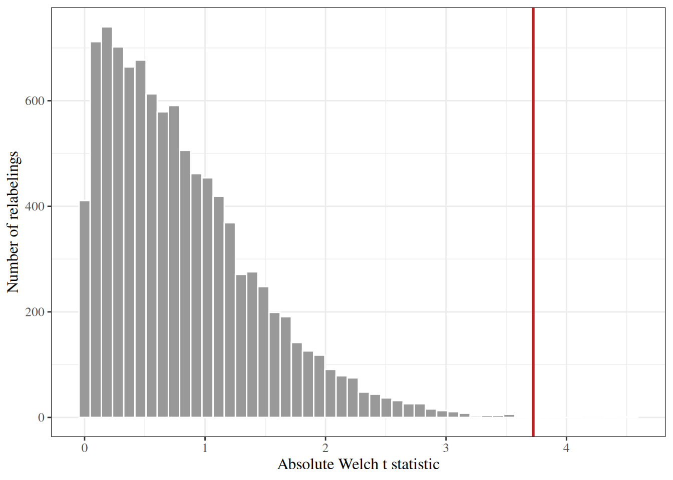
The Monte Carlo error of \(\hat p_{\text{perm}}\) is about \(\sqrt{\hat p_{\text{perm}} (1 - \hat p_{\text{perm}}) / B} =\) 0.00024, which is comparable to the p-value itself, so a p-value this small needs a larger \(B\) before its second digit means anything.
Theorem 2 (The Monte Carlo permutation p-value is valid) Let \(Y\) be exchangeable under \(H_0\) (Definition 1), and let \(\hat p_{\text{perm}}\) be the Monte Carlo permutation p-value of \(T(Y)\) from \(B\) independent uniform permutations. Then \(\hat p_{\text{perm}}\) is a valid p-value:
\[\Pr_{H_0}\mathopen{}\left(\hat p_{\text{perm}} \le u\right)\mathclose{} \le u \quad \text{for every } u \in [0, 1].\]
Remark 2 (Source: The Monte Carlo permutation p-value is valid). Phipson and Smyth [9] show that the Monte Carlo p-value with the added 1 is valid for random permutations. The proof is omitted here.
Example 6 (Validity in a small simulation) Simulate 2000 data sets of 20 independent standard Gaussian values, ten per group, so that \(H_0\) holds. For each, compute \(\hat p_{\text{perm}}\) of the absolute difference in means with \(B = 99\):
set.seed(582)
in_group1 <- rep(c(TRUE, FALSE), each = 10)
abs_diff_means <- function(y, in1) abs(mean(y[in1]) - mean(y[!in1]))
p_hat <- replicate(2000, {
  y <- rnorm(20)
  t_obs <- abs_diff_means(y, in_group1)
  t_perm <- replicate(99, abs_diff_means(y, sample(in_group1)))
  (1 + sum(t_perm >= t_obs)) / 100
})
u <- c(0.01, 0.05, 0.1)
data.frame(
  u = u,
  fraction_p_at_most_u = sapply(u, function(x) mean(p_hat <= x))
)
With \(B = 99\) the p-value takes the values \(0.01, 0.02, \ldots, 1\), and for a statistic with no ties each value has probability \(0.01\) under \(H_0\), so \(\Pr(\hat p_{\text{perm}} \le u) = u\) for \(u\) in that grid. The fractions are close to \(u\), within simulation error. Choosing \(B + 1\) to be a round number such as 100 makes the grid easy to read.
Remark 3 (Why add 1). Without the 1, a data set whose statistic exceeds all \(B\) permuted statistics would get a p-value of 0, which claims that the observed result is impossible under \(H_0\). Under \(H_0\), with no ties, that happens with probability \(1 / (B + 1)\), because the observed statistic is equally likely to be any one of the \(B + 1\) values it is compared with. A p-value that equals 0 with positive probability is not valid. With the 1, the smallest value of \(\hat p_{\text{perm}}\) is \(1 / (B + 1)\).
Hogg et al. [7, Sec. 7.7], pp. 353–360 covers resampling methods.
5 Permutation tests and multiple testing
Example 7 (Permutation p-values for all 2308 genes) Relabeling the samples once permutes every gene at the same time, so \(B = 1000\) relabelings give a permutation null distribution for each of the 2308 genes. This computes \(\mathopen{}\left|t\right|\mathclose{}\) for all genes from column means and sums of squares, in a function checked against t.test() on gene 3:
expr_matrix <- as.matrix(khan_pair[, grepl("^gene_", names(khan_pair))])
abs_welch_t_all <- function(x, in_group1) {
  n1 <- sum(in_group1)
  n2 <- sum(!in_group1)
  mean1 <- colMeans(x[in_group1, , drop = FALSE])
  mean2 <- colMeans(x[!in_group1, , drop = FALSE])
  var1 <- (colSums(x[in_group1, , drop = FALSE]^2) - n1 * mean1^2) / (n1 - 1)
  var2 <- (colSums(x[!in_group1, , drop = FALSE]^2) - n2 * mean2^2) / (n2 - 1)
  abs(mean1 - mean2) / sqrt(var1 / n1 + var2 / n2)
}
t_all <- abs_welch_t_all(expr_matrix, in_class4)
all.equal(unname(t_all["gene_3"]), t_obs)
#> [1] TRUE
Each relabeling yields 2308 statistics, one per gene. The permutation p-value of a gene counts the relabelings whose statistic for that gene reaches its observed one:
B_all <- 1000
set.seed(583)
exceed_counts <- Reduce(
  `+`,
  lapply(seq_len(B_all), function(b) {
    abs_welch_t_all(expr_matrix, sample(in_class4)) >= t_all
  })
)
p_perm_all <- (1 + exceed_counts) / (B_all + 1)
c(
  smallest_possible = 1 / (B_all + 1),
  genes_at_smallest = sum(p_perm_all == 1 / (B_all + 1)),
  bonferroni_threshold = 0.05 / length(p_perm_all)
)
#>    smallest_possible    genes_at_smallest bonferroni_threshold
#>          9.99001e-04          1.36000e+02          2.16638e-05
The smallest p-value that 1000 relabelings can give is 0.001, and 136 genes reach it. The Bonferroni threshold, 0.000022, is far below the smallest possible p-value, so the Bonferroni correction cannot reject any gene with these p-values. For a Bonferroni correction at level \(\alpha\) across \(m\) tests the p-values must be able to fall below \(\alpha/ m\), which needs \(B + 1 \ge m / \alpha\), here \(B \ge\) 46,159 relabelings. The BH procedure needs less resolution, because its thresholds grow with the rank. At \(q = 0.05\) it rejects genes from the permutation p-values and from Welch’s t-test p-values as follows:
welch_p_all <- vapply(
  as.data.frame(expr_matrix),
  function(x) t.test(x ~ khan_pair$tumor_class)$p.value,
  numeric(1)
)
bh_counts <- c(
  permutation = sum(p.adjust(p_perm_all, method = "BH") <= 0.05),
  welch = sum(p.adjust(welch_p_all, method = "BH") <= 0.05)
)
bh_counts
#> permutation       welch
#>         249         250
The two sets of p-values give BH rejection counts of 249 and 250.
6 Further reading
- Good [3] gives a book-length treatment of permutation tests.
- Phipson and Smyth [9] explain why Monte Carlo permutation p-values need the added 1.
- Chapter 12 of the Computational and Inferential Thinking textbook for UC Berkeley’s Data 8 introduces permutation tests through plain-language A/B testing examples.
- Section 24.2 of Lange’s textbook [10] covers permutation tests, with an emphasis on computation.
- Chapter 13 of James et al. [2] applies permutation and other resampling methods to multiple testing.