Convexity in Several Variables

Published

Last modified: 2026-11-13 13:00:00 (PST)

Source

This section is adapted from the convexity part of Zhou [1], used under the MIT License (see the license text in Linear Algebra). The source states the first-order test (in one direction) and the second-derivative test for convexity without proof; here both directions of the first-order test are proved, and the second-derivative test is proved from the Taylor theorem of Section in Critical Points and Optimality Conditions. The source defines both concave and strictly concave as “$-f$ is strictly convex”; here $f$ is concave when $-f$ is convex. The source states that an intersection of convex sets is convex and that a maximum of convex functions is convex for any finite number of them; here each is stated for two and the general case follows by induction. These parts of the source are not part of this section:

its catalogs of convex sets and convex functions, including the positive semidefinite matrices and $-\log \det$
intersections of infinitely many convex sets, and suprema of infinitely many convex functions
its examples, exercises and figures, including the multivariate normal maximum likelihood example

Definition 1 (Convex set)

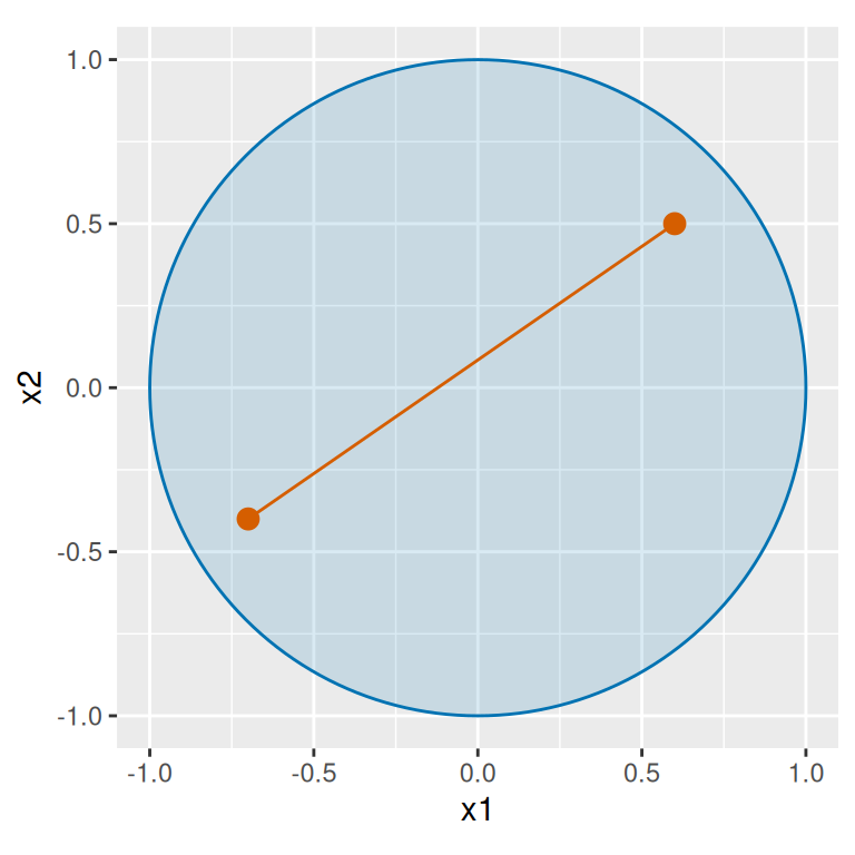
Definition 1 (Convex set) A set $K \subseteq \mathbb{R}^p$ is convex if [2] for all $\mathord{\smash[b]{\underset{\raise.3ex\hbox{$\scriptstyle\sim$}}{x}}\vphantom{x}}, \mathord{\smash[b]{\underset{\raise.3ex\hbox{$\scriptstyle\sim$}}{y}}\vphantom{y}}\in K$ and all $t \in [0, 1]$, the point $t \mathord{\smash[b]{\underset{\raise.3ex\hbox{$\scriptstyle\sim$}}{x}}\vphantom{x}}+ (1 - t) \mathord{\smash[b]{\underset{\raise.3ex\hbox{$\scriptstyle\sim$}}{y}}\vphantom{y}}$ is in $K$: $K$ contains the whole line segment between any two of its points.

Example 1 (Convex sets)

Example 1 (Convex sets)

$\mathbb{R}^p$ is convex, and so is any set with at most one point.
The closed ball $B = \mathopen{}\left\{\mathord{\smash[b]{\underset{\raise.3ex\hbox{$\scriptstyle\sim$}}{x}}\vphantom{x}}: \mathopen{}\left\lVert\mathord{\smash[b]{\underset{\raise.3ex\hbox{$\scriptstyle\sim$}}{x}}\vphantom{x}}\right\rVert\mathclose{} \le r\right\}\mathclose{}$ is convex: for $\mathord{\smash[b]{\underset{\raise.3ex\hbox{$\scriptstyle\sim$}}{x}}\vphantom{x}}, \mathord{\smash[b]{\underset{\raise.3ex\hbox{$\scriptstyle\sim$}}{y}}\vphantom{y}}\in B$ and $t \in [0, 1]$,

\[ \begin{aligned} \mathopen{}\left\lVert t \mathord{\smash[b]{\underset{\raise.3ex\hbox{$\scriptstyle\sim$}}{x}}\vphantom{x}}+ (1 - t) \mathord{\smash[b]{\underset{\raise.3ex\hbox{$\scriptstyle\sim$}}{y}}\vphantom{y}}\right\rVert\mathclose{} &\le \mathopen{}\left\lVert t \mathord{\smash[b]{\underset{\raise.3ex\hbox{$\scriptstyle\sim$}}{x}}\vphantom{x}}\right\rVert\mathclose{} + \mathopen{}\left\lVert(1 - t) \mathord{\smash[b]{\underset{\raise.3ex\hbox{$\scriptstyle\sim$}}{y}}\vphantom{y}}\right\rVert\mathclose{} && \text{(triangle inequality)} \\ &= t\,\mathopen{}\left\lVert\mathord{\smash[b]{\underset{\raise.3ex\hbox{$\scriptstyle\sim$}}{x}}\vphantom{x}}\right\rVert\mathclose{} + (1 - t)\,\mathopen{}\left\lVert\mathord{\smash[b]{\underset{\raise.3ex\hbox{$\scriptstyle\sim$}}{y}}\vphantom{y}}\right\rVert\mathclose{} && \text{(norm of a multiple; } t, 1 - t \ge 0 \text{)} \\ &\le t\,r + (1 - t)\,r && \text{(} \mathord{\smash[b]{\underset{\raise.3ex\hbox{$\scriptstyle\sim$}}{x}}\vphantom{x}}, \mathord{\smash[b]{\underset{\raise.3ex\hbox{$\scriptstyle\sim$}}{y}}\vphantom{y}}\in B \text{)} \\ &= r. && \text{(arithmetic)} \end{aligned} \]

The first step is the triangle inequality, and the second uses the norm of a multiple.

Example 2 (A set that is not convex)

Example 2 (A set that is not convex) $K = \mathopen{}\left\{x \in \mathbb{R}: \mathopen{}\left|x\right|\mathclose{} \ge 1\right\}\mathclose{}$ is not convex: $-1$ and $1$ are in $K$, but with $t = \tfrac{1}{2}$ the point $\tfrac{1}{2}(-1) + \tfrac{1}{2}(1) = 0$ is not.

Show code

cs_angle_fc <- seq(0, 2 * pi, length.out = 201)
cs_cos_fc <- cos(cs_angle_fc)
cs_sin_fc <- sin(cs_angle_fc)
cs_disk_fc <- tibble::tibble(x1 = cs_cos_fc, x2 = cs_sin_fc)
cs_points_x1_fc <- c(-0.7, 0.6)
cs_points_x2_fc <- c(-0.4, 0.5)
cs_points_fc <- tibble::tibble(x1 = cs_points_x1_fc, x2 = cs_points_x2_fc)
cs_segment_fc <- tibble::tibble(
  x1 = -0.7, x2 = -0.4, x1_end = 0.6, x2_end = 0.5
)
cs_aes_fc <- ggplot2::aes(x1, x2)
cs_seg_aes_fc <- ggplot2::aes(xend = x1_end, yend = x2_end)
ggplot2::ggplot(cs_disk_fc, cs_aes_fc) +
  ggplot2::geom_polygon(fill = "#0072B2", alpha = 0.15, colour = "#0072B2") +
  ggplot2::geom_segment(
    data = cs_segment_fc, mapping = cs_seg_aes_fc, colour = "#D55E00"
  ) +
  ggplot2::geom_point(data = cs_points_fc, colour = "#D55E00", size = 3) +
  ggplot2::coord_fixed() +
  ggplot2::labs(x = "x1", y = "x2")

Show code

import matplotlib.pyplot as plt
import numpy as np

cs_angle_fc = np.linspace(0, 2 * np.pi, 201)
cs_x1_fc = np.array([-0.7, 0.6])
cs_x2_fc = np.array([-0.4, 0.5])
fig, ax = plt.subplots(figsize=(4, 4), layout="constrained")
ax.fill(np.cos(cs_angle_fc), np.sin(cs_angle_fc), color="#0072B2", alpha=0.15)
ax.plot(np.cos(cs_angle_fc), np.sin(cs_angle_fc), color="#0072B2")
ax.plot(cs_x1_fc, cs_x2_fc, "o-", color="#D55E00", markersize=8)
ax.set_aspect("equal")
ax.set_xlabel("x1")
ax.set_ylabel("x2")
plt.show()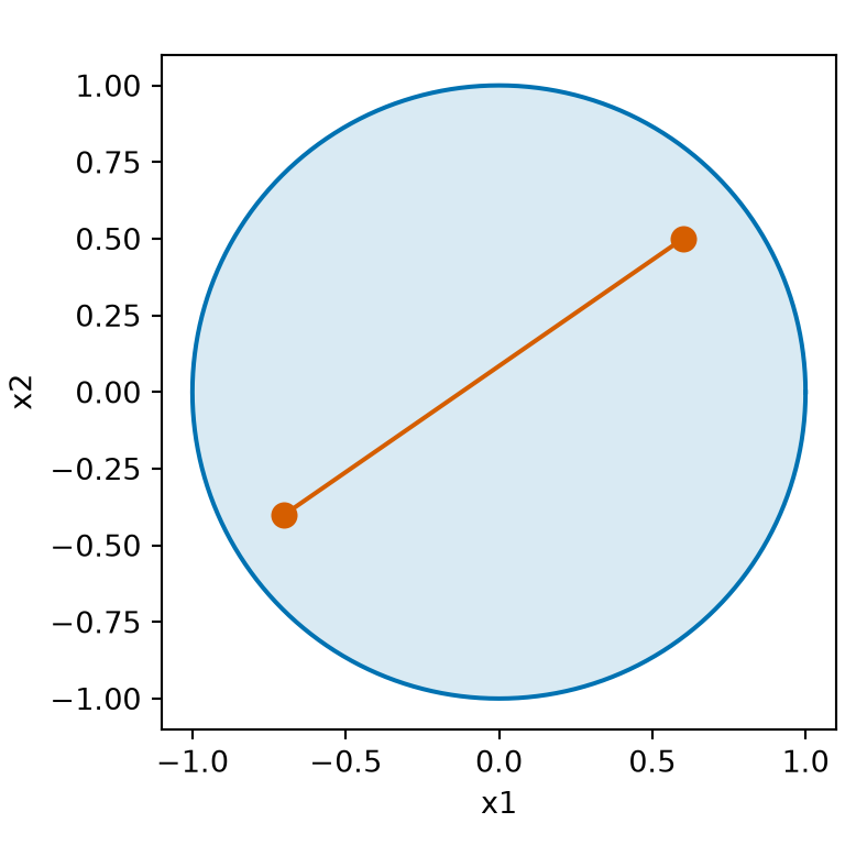

A blue-outlined disk of radius 1 centered at the origin, shaded light blue. Two vermilion circles mark points x and y inside it, joined by a vermilion segment that stays inside the disk. — Figure 1: The closed ball of Example 1 in $\mathbb{R}^2$ with $r = 1$. The segment between two of its points stays in the ball, as a convex set requires.

Definition 2 (Half-space)

Definition 2 (Half-space) Let $\mathord{\smash[b]{\underset{\raise.3ex\hbox{$\scriptstyle\sim$}}{a}}\vphantom{a}} \in \mathbb{R}^p$ be a nonzero vector and $c$ a real number. The set $\mathopen{}\left\{\mathord{\smash[b]{\underset{\raise.3ex\hbox{$\scriptstyle\sim$}}{x}}\vphantom{x}}\in \mathbb{R}^p : \mathord{\smash[b]{\underset{\raise.3ex\hbox{$\scriptstyle\sim$}}{a}}\vphantom{a}} \cdot \mathord{\smash[b]{\underset{\raise.3ex\hbox{$\scriptstyle\sim$}}{x}}\vphantom{x}} \ge c\right\}\mathclose{}$ is a (closed) half-space: the points on one side of the boundary $\mathopen{}\left\{\mathord{\smash[b]{\underset{\raise.3ex\hbox{$\scriptstyle\sim$}}{x}}\vphantom{x}}: \mathord{\smash[b]{\underset{\raise.3ex\hbox{$\scriptstyle\sim$}}{a}}\vphantom{a}} \cdot \mathord{\smash[b]{\underset{\raise.3ex\hbox{$\scriptstyle\sim$}}{x}}\vphantom{x}} = c\right\}\mathclose{}$, together with the boundary. In $\mathbb{R}^2$, a half-space is called a half-plane.

Example 3 (The right half-plane)

Example 3 (The right half-plane) With $\mathord{\smash[b]{\underset{\raise.3ex\hbox{$\scriptstyle\sim$}}{a}}\vphantom{a}} = {(1, 0)}^{\top}$ and $c = 0$, the half-plane $\mathopen{}\left\{\mathord{\smash[b]{\underset{\raise.3ex\hbox{$\scriptstyle\sim$}}{x}}\vphantom{x}}\in \mathbb{R}^2 : x_1 \ge 0\right\}\mathclose{}$ is the set of points on or to the right of the $x_2$-axis. ${(1, 5)}^{\top}$ is in it, since $1 \ge 0$; ${(0, -3)}^{\top}$ is in it, on the boundary; and ${(-1, 0)}^{\top}$ is not, since $-1 < 0$.

Theorem 1 (An intersection of convex sets is convex)

Theorem 1 (An intersection of convex sets is convex) If $K_1$ and $K_2$ are convex subsets of $\mathbb{R}^p$ (Definition 1), then $K_1 \cap K_2$ is convex.

Proof

Proof. Let $\mathord{\smash[b]{\underset{\raise.3ex\hbox{$\scriptstyle\sim$}}{x}}\vphantom{x}}, \mathord{\smash[b]{\underset{\raise.3ex\hbox{$\scriptstyle\sim$}}{y}}\vphantom{y}}\in K_1 \cap K_2$ and $t \in [0, 1]$. Then $\mathord{\smash[b]{\underset{\raise.3ex\hbox{$\scriptstyle\sim$}}{x}}\vphantom{x}}, \mathord{\smash[b]{\underset{\raise.3ex\hbox{$\scriptstyle\sim$}}{y}}\vphantom{y}}\in K_1$, so $t \mathord{\smash[b]{\underset{\raise.3ex\hbox{$\scriptstyle\sim$}}{x}}\vphantom{x}}+ (1 - t) \mathord{\smash[b]{\underset{\raise.3ex\hbox{$\scriptstyle\sim$}}{y}}\vphantom{y}}\in K_1$, since $K_1$ is convex; in the same way $t \mathord{\smash[b]{\underset{\raise.3ex\hbox{$\scriptstyle\sim$}}{x}}\vphantom{x}}+ (1 - t) \mathord{\smash[b]{\underset{\raise.3ex\hbox{$\scriptstyle\sim$}}{y}}\vphantom{y}}\in K_2$. So $t \mathord{\smash[b]{\underset{\raise.3ex\hbox{$\scriptstyle\sim$}}{x}}\vphantom{x}}+ (1 - t) \mathord{\smash[b]{\underset{\raise.3ex\hbox{$\scriptstyle\sim$}}{y}}\vphantom{y}}\in K_1 \cap K_2$.

Example 4 (Intersecting a ball with a half-plane)

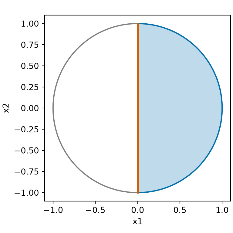
Example 4 (Intersecting a ball with a half-plane) The closed unit ball in $\mathbb{R}^2$ is convex (Example 1), and so is the half-plane (Definition 2) $\mathopen{}\left\{\mathord{\smash[b]{\underset{\raise.3ex\hbox{$\scriptstyle\sim$}}{x}}\vphantom{x}}: x_1 \ge 0\right\}\mathclose{}$: if $x_1 \ge 0$ and $y_1 \ge 0$, then $t x_1 + (1 - t) y_1 \ge 0$ for $t \in [0, 1]$. By Theorem 1, the closed half-disk $\mathopen{}\left\{\mathord{\smash[b]{\underset{\raise.3ex\hbox{$\scriptstyle\sim$}}{x}}\vphantom{x}}: \mathopen{}\left\lVert\mathord{\smash[b]{\underset{\raise.3ex\hbox{$\scriptstyle\sim$}}{x}}\vphantom{x}}\right\rVert\mathclose{} \le 1,\ x_1 \ge 0\right\}\mathclose{}$ is convex. A union need not be convex: $\mathopen{}\left\{x \in \mathbb{R}: x \le -1\right\}\mathclose{}$ and $\mathopen{}\left\{x \in \mathbb{R}: x \ge 1\right\}\mathclose{}$ are convex, but their union is the set of Example 2.

Figure 2 shows the half-disk.

Show code

ci_angle_ci <- seq(-pi / 2, pi / 2, length.out = 101)
ci_half_x1_ci <- cos(ci_angle_ci)
ci_half_x2_ci <- sin(ci_angle_ci)
ci_half_ci <- tibble::tibble(x1 = ci_half_x1_ci, x2 = ci_half_x2_ci)
ci_full_angle_ci <- seq(0, 2 * pi, length.out = 201)
ci_full_x1_ci <- cos(ci_full_angle_ci)
ci_full_x2_ci <- sin(ci_full_angle_ci)
ci_full_ci <- tibble::tibble(x1 = ci_full_x1_ci, x2 = ci_full_x2_ci)
ci_edge_ci <- tibble::tibble(x1 = 0, x2 = -1, x1_end = 0, x2_end = 1)
ci_aes_ci <- ggplot2::aes(x1, x2)
ci_seg_aes_ci <- ggplot2::aes(xend = x1_end, yend = x2_end)
ci_full_ci |>
  ggplot2::ggplot() +
  ci_aes_ci +
  ggplot2::geom_path(colour = "grey60") +
  ggplot2::geom_polygon(
    data = ci_half_ci, fill = "#0072B2", alpha = 0.25, colour = "#0072B2"
  ) +
  ggplot2::geom_segment(
    data = ci_edge_ci, mapping = ci_seg_aes_ci,
    colour = "#D55E00", linewidth = 1
  ) +
  ggplot2::coord_fixed() +
  ggplot2::labs(x = "x1", y = "x2")

Show code

import matplotlib.pyplot as plt
import numpy as np

ci_full_py = np.linspace(0, 2 * np.pi, 201)
ci_half_py = np.linspace(-np.pi / 2, np.pi / 2, 101)
fig, ax = plt.subplots(figsize=(4, 4), layout="constrained")
ax.plot(np.cos(ci_full_py), np.sin(ci_full_py), color="grey")
ax.fill(np.cos(ci_half_py), np.sin(ci_half_py), color="#0072B2", alpha=0.25)
ax.plot(np.cos(ci_half_py), np.sin(ci_half_py), color="#0072B2")
ax.plot([0, 0], [-1, 1], color="#D55E00", linewidth=2)
ax.set_aspect("equal")
ax.set_xlabel("x1")
ax.set_ylabel("x2")
plt.show();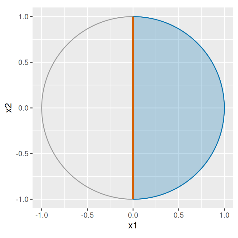

A circle of radius 1 centered at the origin, drawn as a grey outline, with the right half of the disk, where x1 is at least 0, shaded blue and outlined in blue. A vermilion vertical segment along the x2 axis from -1 to 1 marks the edge of the half-plane x1 equal to 0. — Figure 2: The closed half-disk (blue) is the intersection of the unit ball with the half-plane $x_1 \ge 0$ of Example 4. The vermilion segment is the edge of the half-plane. The half-disk is convex, as Theorem 1 states.

Definition 3 (Convex hull, convex envelope)

Definition 3 (Convex hull, convex envelope) The convex hull (or convex envelope) [3] of a set $S \subseteq \mathbb{R}^p$ is the set of points that lie in every convex set containing $S$:

\[ \operatorname{conv}(S) \stackrel{\text{def}}{=}\mathopen{}\left\{\mathord{\smash[b]{\underset{\raise.3ex\hbox{$\scriptstyle\sim$}}{x}}\vphantom{x}}\in \mathbb{R}^p : \mathord{\smash[b]{\underset{\raise.3ex\hbox{$\scriptstyle\sim$}}{x}}\vphantom{x}}\in K \text{ for every convex } K \subseteq \mathbb{R}^p \text{ with } S \subseteq K\right\}\mathclose{}. \]

Example 5 (The convex hull of three points is a triangle)

Example 5 (The convex hull of three points is a triangle) Let $S = \mathopen{}\left\{\mathord{\smash[b]{\underset{\raise.3ex\hbox{$\scriptstyle\sim$}}{0}}\vphantom{0}}, \mathord{\smash[b]{\underset{\raise.3ex\hbox{$\scriptstyle\sim$}}{e}}\vphantom{e}}_1, \mathord{\smash[b]{\underset{\raise.3ex\hbox{$\scriptstyle\sim$}}{e}}\vphantom{e}}_2\right\}\mathclose{} \subseteq \mathbb{R}^2$, with $\mathord{\smash[b]{\underset{\raise.3ex\hbox{$\scriptstyle\sim$}}{e}}\vphantom{e}}_1 = {(1, 0)}^{\top}$ and $\mathord{\smash[b]{\underset{\raise.3ex\hbox{$\scriptstyle\sim$}}{e}}\vphantom{e}}_2 = {(0, 1)}^{\top}$, and let $T = \mathopen{}\left\{\mathord{\smash[b]{\underset{\raise.3ex\hbox{$\scriptstyle\sim$}}{x}}\vphantom{x}}\in \mathbb{R}^2 : x_1 \ge 0,\ x_2 \ge 0,\ x_1 + x_2 \le 1\right\}\mathclose{}$, the filled triangle with corners $\mathord{\smash[b]{\underset{\raise.3ex\hbox{$\scriptstyle\sim$}}{0}}\vphantom{0}}$, $\mathord{\smash[b]{\underset{\raise.3ex\hbox{$\scriptstyle\sim$}}{e}}\vphantom{e}}_1$ and $\mathord{\smash[b]{\underset{\raise.3ex\hbox{$\scriptstyle\sim$}}{e}}\vphantom{e}}_2$. Then $\operatorname{conv}(S) = T$: the convex hull of $S$ is $T$.

Inclusion $\operatorname{conv}(S) \subseteq T$. $T$ is the intersection of three half-planes, with $\mathord{\smash[b]{\underset{\raise.3ex\hbox{$\scriptstyle\sim$}}{a}}\vphantom{a}} = {(1, 0)}^{\top}$, ${(0, 1)}^{\top}$ and ${(-1, -1)}^{\top}$, and $c = 0$, $0$ and $-1$. Each half-plane $H = \mathopen{}\left\{\mathord{\smash[b]{\underset{\raise.3ex\hbox{$\scriptstyle\sim$}}{x}}\vphantom{x}}: \mathord{\smash[b]{\underset{\raise.3ex\hbox{$\scriptstyle\sim$}}{a}}\vphantom{a}} \cdot \mathord{\smash[b]{\underset{\raise.3ex\hbox{$\scriptstyle\sim$}}{x}}\vphantom{x}} \ge c\right\}\mathclose{}$ is convex: for $\mathord{\smash[b]{\underset{\raise.3ex\hbox{$\scriptstyle\sim$}}{x}}\vphantom{x}}, \mathord{\smash[b]{\underset{\raise.3ex\hbox{$\scriptstyle\sim$}}{y}}\vphantom{y}}\in H$ and $t \in [0, 1]$,

\[ \begin{aligned} \mathord{\smash[b]{\underset{\raise.3ex\hbox{$\scriptstyle\sim$}}{a}}\vphantom{a}} \cdot t \mathord{\smash[b]{\underset{\raise.3ex\hbox{$\scriptstyle\sim$}}{x}}\vphantom{x}}+ (1 - t) \mathord{\smash[b]{\underset{\raise.3ex\hbox{$\scriptstyle\sim$}}{y}}\vphantom{y}} &= t \mathord{\smash[b]{\underset{\raise.3ex\hbox{$\scriptstyle\sim$}}{a}}\vphantom{a}} \cdot \mathord{\smash[b]{\underset{\raise.3ex\hbox{$\scriptstyle\sim$}}{x}}\vphantom{x}} + (1 - t) \mathord{\smash[b]{\underset{\raise.3ex\hbox{$\scriptstyle\sim$}}{a}}\vphantom{a}} \cdot \mathord{\smash[b]{\underset{\raise.3ex\hbox{$\scriptstyle\sim$}}{y}}\vphantom{y}} && \text{(the dot product is linear)} \\ &\ge t c + (1 - t) c && \text{(} \mathord{\smash[b]{\underset{\raise.3ex\hbox{$\scriptstyle\sim$}}{x}}\vphantom{x}}, \mathord{\smash[b]{\underset{\raise.3ex\hbox{$\scriptstyle\sim$}}{y}}\vphantom{y}}\in H \text{ and } t, 1 - t \ge 0 \text{)} \\ &= c. && \text{(arithmetic)} \end{aligned} \]

So $T$ is convex, by Theorem 1 applied twice. $T$ contains $S$, so every point of $\operatorname{conv}(S)$ is in $T$.
Inclusion $T \subseteq \operatorname{conv}(S)$. Let $K$ be a convex set containing $S$, let $\mathord{\smash[b]{\underset{\raise.3ex\hbox{$\scriptstyle\sim$}}{x}}\vphantom{x}}\in T$, and let $s = x_1 + x_2$, so $0 \le s \le 1$. If $s = 0$, then $\mathord{\smash[b]{\underset{\raise.3ex\hbox{$\scriptstyle\sim$}}{x}}\vphantom{x}}= \mathord{\smash[b]{\underset{\raise.3ex\hbox{$\scriptstyle\sim$}}{0}}\vphantom{0}}\in K$. Otherwise $\mathord{\smash[b]{\underset{\raise.3ex\hbox{$\scriptstyle\sim$}}{p}}\vphantom{p}} = \mathord{\smash[b]{\underset{\raise.3ex\hbox{$\scriptstyle\sim$}}{x}}\vphantom{x}}/ s$ has $p_1 + p_2 = 1$ with $p_1, p_2 \ge 0$, so $\mathord{\smash[b]{\underset{\raise.3ex\hbox{$\scriptstyle\sim$}}{p}}\vphantom{p}} = p_1 \mathord{\smash[b]{\underset{\raise.3ex\hbox{$\scriptstyle\sim$}}{e}}\vphantom{e}}_1 + (1 - p_1) \mathord{\smash[b]{\underset{\raise.3ex\hbox{$\scriptstyle\sim$}}{e}}\vphantom{e}}_2$ is in $K$, by convexity with $t = p_1$. Then $\mathord{\smash[b]{\underset{\raise.3ex\hbox{$\scriptstyle\sim$}}{x}}\vphantom{x}}= s \mathord{\smash[b]{\underset{\raise.3ex\hbox{$\scriptstyle\sim$}}{p}}\vphantom{p}} + (1 - s) \mathord{\smash[b]{\underset{\raise.3ex\hbox{$\scriptstyle\sim$}}{0}}\vphantom{0}}$ is in $K$, by convexity with $t = s$. So $\mathord{\smash[b]{\underset{\raise.3ex\hbox{$\scriptstyle\sim$}}{x}}\vphantom{x}}$ is in every convex set containing $S$.

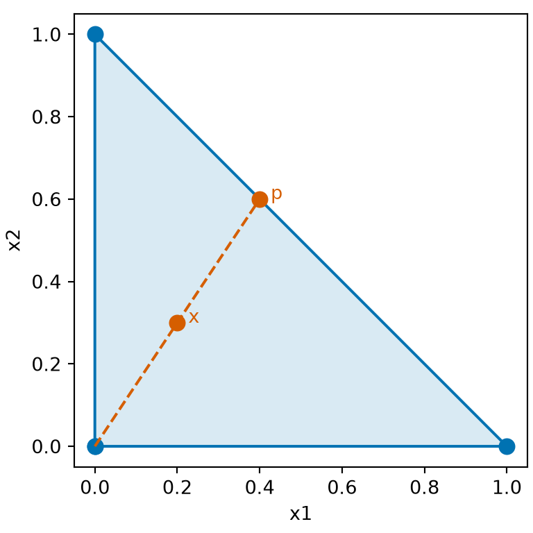
Figure 3 shows $S$, $T$ and the two steps for one point of $T$.

Show code

ch_corner_x1_fc <- c(0, 1, 0)
ch_corner_x2_fc <- c(0, 0, 1)
ch_corners_fc <- tibble::tibble(x1 = ch_corner_x1_fc, x2 = ch_corner_x2_fc)
ch_path_x1_fc <- c(0, 0.2, 0.4)
ch_path_x2_fc <- c(0, 0.3, 0.6)
ch_path_fc <- tibble::tibble(x1 = ch_path_x1_fc, x2 = ch_path_x2_fc)
ch_marks_x1_fc <- c(0.2, 0.4)
ch_marks_x2_fc <- c(0.3, 0.6)
ch_marks_label_fc <- c("x", "p")
ch_marks_fc <- tibble::tibble(
  x1 = ch_marks_x1_fc,
  x2 = ch_marks_x2_fc,
  label = ch_marks_label_fc
)
ch_aes_fc <- ggplot2::aes(x = x1, y = x2)
ch_label_aes_fc <- ggplot2::aes(x = x1, y = x2, label = label)
ggplot2::ggplot() +
  ggplot2::geom_polygon(
    data = ch_corners_fc, mapping = ch_aes_fc,
    fill = "#0072B2", alpha = 0.15, colour = "#0072B2"
  ) +
  ggplot2::geom_point(
    data = ch_corners_fc, mapping = ch_aes_fc,
    colour = "#0072B2", size = 3
  ) +
  ggplot2::geom_line(
    data = ch_path_fc, mapping = ch_aes_fc,
    colour = "#D55E00", linetype = "dashed"
  ) +
  ggplot2::geom_point(
    data = ch_marks_fc, mapping = ch_aes_fc,
    colour = "#D55E00", size = 3
  ) +
  ggplot2::geom_text(
    data = ch_marks_fc, mapping = ch_label_aes_fc,
    colour = "#D55E00", nudge_x = 0.07
  ) +
  ggplot2::coord_fixed() +
  ggplot2::labs(x = "x1", y = "x2")

Show code

import matplotlib.pyplot as plt

ch_x1_fc = [0, 1, 0]
ch_x2_fc = [0, 0, 1]
fig, ax = plt.subplots(figsize=(4, 4), layout="constrained")
ax.fill(ch_x1_fc, ch_x2_fc, color="#0072B2", alpha=0.15);
ax.plot(ch_x1_fc + [0], ch_x2_fc + [0], "o-", color="#0072B2", markersize=8);
ax.plot([0, 0.4], [0, 0.6], "--", color="#D55E00");
ax.plot([0.2, 0.4], [0.3, 0.6], "o", color="#D55E00", markersize=8);
ax.annotate("x", (0.2, 0.3), xytext=(6, 0), textcoords="offset points",
            color="#D55E00");
ax.annotate("p", (0.4, 0.6), xytext=(6, 0), textcoords="offset points",
            color="#D55E00");
ax.set_aspect("equal");
ax.set_xlabel("x1");
ax.set_ylabel("x2");
plt.show();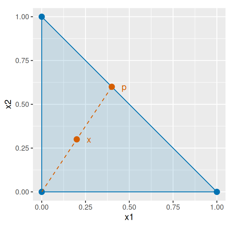

A light blue filled triangle with blue corners at (0, 0), (1, 0) and (0, 1). A vermilion point p at (0.4, 0.6) sits on the edge from (1, 0) to (0, 1). A dashed vermilion segment runs from the origin to p, passing through a second vermilion point x at (0.2, 0.3), halfway along it. — Figure 3: The three blue corners are the set $S$ of Example 5. The shaded triangle $T$ is its convex hull. The point $\mathord{\smash[b]{\underset{\raise.3ex\hbox{$\scriptstyle\sim$}}{x}}\vphantom{x}}= {(0.2, 0.3)}^{\top}$ has $s = 0.5$. The point $\mathord{\smash[b]{\underset{\raise.3ex\hbox{$\scriptstyle\sim$}}{p}}\vphantom{p}} = {(0.4, 0.6)}^{\top}$ lies on the segment between $\mathord{\smash[b]{\underset{\raise.3ex\hbox{$\scriptstyle\sim$}}{e}}\vphantom{e}}_1$ and $\mathord{\smash[b]{\underset{\raise.3ex\hbox{$\scriptstyle\sim$}}{e}}\vphantom{e}}_2$, and $\mathord{\smash[b]{\underset{\raise.3ex\hbox{$\scriptstyle\sim$}}{x}}\vphantom{x}}$ lies on the segment between $\mathord{\smash[b]{\underset{\raise.3ex\hbox{$\scriptstyle\sim$}}{0}}\vphantom{0}}$ and $\mathord{\smash[b]{\underset{\raise.3ex\hbox{$\scriptstyle\sim$}}{p}}\vphantom{p}}$.

Definition 4 (Strictly convex function)

Definition 4 (Strictly convex function) A function $f : \mathbb{R}^p \to \mathbb{R}$ is strictly convex if $f(t \mathord{\smash[b]{\underset{\raise.3ex\hbox{$\scriptstyle\sim$}}{x}}\vphantom{x}}+ (1 - t) \mathord{\smash[b]{\underset{\raise.3ex\hbox{$\scriptstyle\sim$}}{y}}\vphantom{y}}) < t f(\mathord{\smash[b]{\underset{\raise.3ex\hbox{$\scriptstyle\sim$}}{x}}\vphantom{x}}) + (1 - t) f(\mathord{\smash[b]{\underset{\raise.3ex\hbox{$\scriptstyle\sim$}}{y}}\vphantom{y}})$ for all $\mathord{\smash[b]{\underset{\raise.3ex\hbox{$\scriptstyle\sim$}}{x}}\vphantom{x}}\ne \mathord{\smash[b]{\underset{\raise.3ex\hbox{$\scriptstyle\sim$}}{y}}\vphantom{y}}$ in $\mathbb{R}^p$ and all $t \in (0, 1)$.

Definition 5 (Concave function)

Definition 5 (Concave function) A function $f : \mathbb{R}^p \to \mathbb{R}$ is concave if $-f$ is convex.

Definition 6 (Strictly concave function)

Definition 6 (Strictly concave function) A function $f : \mathbb{R}^p \to \mathbb{R}$ is strictly concave if $-f$ is strictly convex (Definition 4).

Example 6 (Strictly convex, and convex but not strictly)

Example 6 (Strictly convex, and convex but not strictly)

$f(x) = x^2$ is strictly convex:

\[ \begin{aligned} t x^2 + (1 - t) y^2 - (t x + (1 - t) y)^2 &= t x^2 + (1 - t) y^2 - t^2 x^2 - 2 t (1 - t) x y - (1 - t)^2 y^2 && \text{(expand the square)} \\ &= t (1 - t) x^2 - 2 t (1 - t) x y + t (1 - t) y^2 && \text{(} t - t^2 = t (1 - t) \text{, } (1 - t) - (1 - t)^2 = t (1 - t) \text{)} \\ &= t (1 - t) (x - y)^2, && \text{(factor)} \end{aligned} \]

which is positive when $x \ne y$ and $t \in (0, 1)$. At $t \in \mathopen{}\left\{0, 1\right\}\mathclose{}$ or $x = y$ it is $0$, so $x^2$ is also convex.
$f(x) = 2x + 1$ is convex but not strictly convex:

\[ \begin{aligned} f(t x + (1 - t) y) &= 2 t x + 2 (1 - t) y + 1 \\ &= t f(x) + (1 - t) f(y) \end{aligned} \]

for every $x, y, t$, so the inequality holds, but never strictly. It is also concave.

Theorem 2 (An open ball is convex)

Theorem 2 (An open ball is convex) Let $\mathord{\smash[b]{\underset{\raise.3ex\hbox{$\scriptstyle\sim$}}{x}}\vphantom{x}}_0 \in \mathbb{R}^p$ and $r > 0$. The open ball of radius $r$ around $\mathord{\smash[b]{\underset{\raise.3ex\hbox{$\scriptstyle\sim$}}{x}}\vphantom{x}}_0$ is a convex set.

Proof

Proof. Call the open ball $B$, and let $\mathord{\smash[b]{\underset{\raise.3ex\hbox{$\scriptstyle\sim$}}{x}}\vphantom{x}}, \mathord{\smash[b]{\underset{\raise.3ex\hbox{$\scriptstyle\sim$}}{y}}\vphantom{y}}\in B$ and $t \in [0, 1]$. The triangle inequality and the absolute homogeneity of the norm give

\[ \begin{aligned} \mathopen{}\left\lVert t \mathord{\smash[b]{\underset{\raise.3ex\hbox{$\scriptstyle\sim$}}{x}}\vphantom{x}}+ (1 - t) \mathord{\smash[b]{\underset{\raise.3ex\hbox{$\scriptstyle\sim$}}{y}}\vphantom{y}}- \mathord{\smash[b]{\underset{\raise.3ex\hbox{$\scriptstyle\sim$}}{x}}\vphantom{x}}_0\right\rVert\mathclose{} &= \mathopen{}\left\lVert t (\mathord{\smash[b]{\underset{\raise.3ex\hbox{$\scriptstyle\sim$}}{x}}\vphantom{x}}- \mathord{\smash[b]{\underset{\raise.3ex\hbox{$\scriptstyle\sim$}}{x}}\vphantom{x}}_0) + (1 - t) (\mathord{\smash[b]{\underset{\raise.3ex\hbox{$\scriptstyle\sim$}}{y}}\vphantom{y}}- \mathord{\smash[b]{\underset{\raise.3ex\hbox{$\scriptstyle\sim$}}{x}}\vphantom{x}}_0)\right\rVert\mathclose{} && \text{(} \mathord{\smash[b]{\underset{\raise.3ex\hbox{$\scriptstyle\sim$}}{x}}\vphantom{x}}_0 = t \mathord{\smash[b]{\underset{\raise.3ex\hbox{$\scriptstyle\sim$}}{x}}\vphantom{x}}_0 + (1 - t) \mathord{\smash[b]{\underset{\raise.3ex\hbox{$\scriptstyle\sim$}}{x}}\vphantom{x}}_0 \text{)} \\ &\le t \mathopen{}\left\lVert\mathord{\smash[b]{\underset{\raise.3ex\hbox{$\scriptstyle\sim$}}{x}}\vphantom{x}}- \mathord{\smash[b]{\underset{\raise.3ex\hbox{$\scriptstyle\sim$}}{x}}\vphantom{x}}_0\right\rVert\mathclose{} + (1 - t) \mathopen{}\left\lVert\mathord{\smash[b]{\underset{\raise.3ex\hbox{$\scriptstyle\sim$}}{y}}\vphantom{y}}- \mathord{\smash[b]{\underset{\raise.3ex\hbox{$\scriptstyle\sim$}}{x}}\vphantom{x}}_0\right\rVert\mathclose{} && \text{(triangle inequality and } t, 1 - t \ge 0 \text{)} \\ &< r, && \text{(weighted mean of two numbers less than } r \text{)} \end{aligned} \]

so $t \mathord{\smash[b]{\underset{\raise.3ex\hbox{$\scriptstyle\sim$}}{x}}\vphantom{x}}+ (1 - t) \mathord{\smash[b]{\underset{\raise.3ex\hbox{$\scriptstyle\sim$}}{y}}\vphantom{y}}\in B$.

Definition 7 (Convex function on a set)

Definition 7 (Convex function on a set) Let $K \subseteq \mathbb{R}^p$ be a convex set. A function $f : \mathbb{R}^p \to \mathbb{R}$ is convex on $K$ if

\[ f(t \mathord{\smash[b]{\underset{\raise.3ex\hbox{$\scriptstyle\sim$}}{x}}\vphantom{x}}+ (1 - t) \mathord{\smash[b]{\underset{\raise.3ex\hbox{$\scriptstyle\sim$}}{y}}\vphantom{y}}) \le t f(\mathord{\smash[b]{\underset{\raise.3ex\hbox{$\scriptstyle\sim$}}{x}}\vphantom{x}}) + (1 - t) f(\mathord{\smash[b]{\underset{\raise.3ex\hbox{$\scriptstyle\sim$}}{y}}\vphantom{y}}) \]

for all $\mathord{\smash[b]{\underset{\raise.3ex\hbox{$\scriptstyle\sim$}}{x}}\vphantom{x}}, \mathord{\smash[b]{\underset{\raise.3ex\hbox{$\scriptstyle\sim$}}{y}}\vphantom{y}}\in K$ and all $t \in [0, 1]$.

Example 7 (A function convex on an interval but not on the whole line)

Example 7 (A function convex on an interval but not on the whole line) Let $f(x) = {\min\mathopen{}\left(x^2, 1\right)\mathclose{}}$.

$f$ is convex on $[-1, 1]$, which is the closed ball of radius $1$ around $0$ and so convex by Example 1. For $x, y \in [-1, 1]$ and $t \in [0, 1]$, the point $t x + (1 - t) y$ is also in $[-1, 1]$, where $f$ agrees with $x^2$, so the defining inequality of $f$ is the defining inequality of $x^2$, which holds by Example 6.
$f$ is not convex on all of $\mathbb{R}$: with $x = 0$, $y = 2$ and $t = \tfrac{1}{2}$,

\[ \begin{aligned} f\mathopen{}\left(\tfrac{1}{2} \cdot 0 + \tfrac{1}{2} \cdot 2\right)\mathclose{} &= f(1) && \text{(} \tfrac{1}{2} \cdot 0 + \tfrac{1}{2} \cdot 2 = 1 \text{)} \\ &= 1, && \text{(} {\min\mathopen{}\left(1, 1\right)\mathclose{}} = 1 \text{)} \end{aligned} \]

which is greater than $\tfrac{1}{2} f(0) + \tfrac{1}{2} f(2) = \tfrac{1}{2}$, since $f(0) = 0$ and $f(2) = 1$.

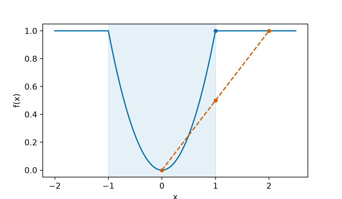
In Figure 4, the chord from $0$ to $2$ passes below the graph at $1$, while every chord with both ends in $[-1, 1]$ lies on or above it.

Show code

co_x_co <- seq(-2, 2.5, length.out = 451)
co_square_co <- co_x_co^2
co_f_co <- pmin(co_square_co, 1)
co_graph_co <- tibble::tibble(x = co_x_co, f = co_f_co)
co_chord_x_co <- c(0, 2)
co_chord_f_co <- c(0, 1)
co_chord_co <- tibble::tibble(x = co_chord_x_co, f = co_chord_f_co)
co_mid_x_co <- c(1, 1)
co_mid_f_co <- c(0.5, 1)
co_mid_co <- tibble::tibble(x = co_mid_x_co, f = co_mid_f_co)
co_mid_cols_co <- c("#D55E00", "#0072B2")
co_graph_co |>
  ggplot2::ggplot() +
  ggplot2::aes(x = x, y = f) +
  ggplot2::annotate(
    "rect",
    xmin = -1, xmax = 1, ymin = -Inf, ymax = Inf,
    fill = "#0072B2", alpha = 0.1
  ) +
  ggplot2::geom_line(colour = "#0072B2") +
  ggplot2::geom_line(
    data = co_chord_co, colour = "#D55E00", linetype = "dashed"
  ) +
  ggplot2::geom_point(data = co_chord_co, colour = "#D55E00", size = 2) +
  ggplot2::geom_point(data = co_mid_co, colour = co_mid_cols_co, size = 2) +
  ggplot2::labs(x = "x", y = "f(x)") +
  ggplot2::theme_minimal()

Show code

import matplotlib.pyplot as plt
import numpy as np

co_x_py = np.linspace(-2, 2.5, 451)
co_f_py = np.minimum(co_x_py**2, 1)
fig, ax = plt.subplots(figsize=(6, 3.5))
ax.axvspan(-1, 1, color="#0072B2", alpha=0.1)
ax.plot(co_x_py, co_f_py, color="#0072B2")
ax.plot([0, 2], [0, 1], "--o", color="#D55E00", markersize=4)
ax.plot([1], [0.5], "o", color="#D55E00", markersize=4)
ax.plot([1], [1], "o", color="#0072B2", markersize=4)
ax.set_xlabel("x")
ax.set_ylabel("f(x)")
plt.show();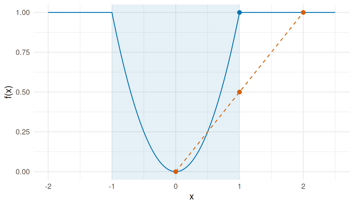

The graph of f(x) = min(x^2, 1) for x from -2 to 2.5: a parabola between -1 and 1, flat at height 1 outside. The interval from -1 to 1 is shaded. A dashed vermilion chord joins (0, 0) and (2, 1) and passes through (1, 0.5), below the graph's value 1 at x = 1. — Figure 4: The graph of $f(x) = {\min\mathopen{}\left(x^2, 1\right)\mathclose{}}$ from Example 7. On the shaded interval $[-1, 1]$, $f$ is $x^2$ and is convex on it. The dashed chord from $0$ to $2$ is at $\tfrac{1}{2}$ above $x = 1$, below $f(1) = 1$.

Definition 8 (Function convex at a point)

Definition 8 (Function convex at a point) Let $f : \mathbb{R}^p \to \mathbb{R}$ and let $\mathord{\smash[b]{\underset{\raise.3ex\hbox{$\scriptstyle\sim$}}{x}}\vphantom{x}}_0 \in \mathbb{R}^p$. $f$ is convex at $\mathord{\smash[b]{\underset{\raise.3ex\hbox{$\scriptstyle\sim$}}{x}}\vphantom{x}}_0$ if there is an $r > 0$ such that $f$ is convex on the open ball of radius $r$ around $\mathord{\smash[b]{\underset{\raise.3ex\hbox{$\scriptstyle\sim$}}{x}}\vphantom{x}}_0$.

Example 8 (A function convex at one point and not at another)

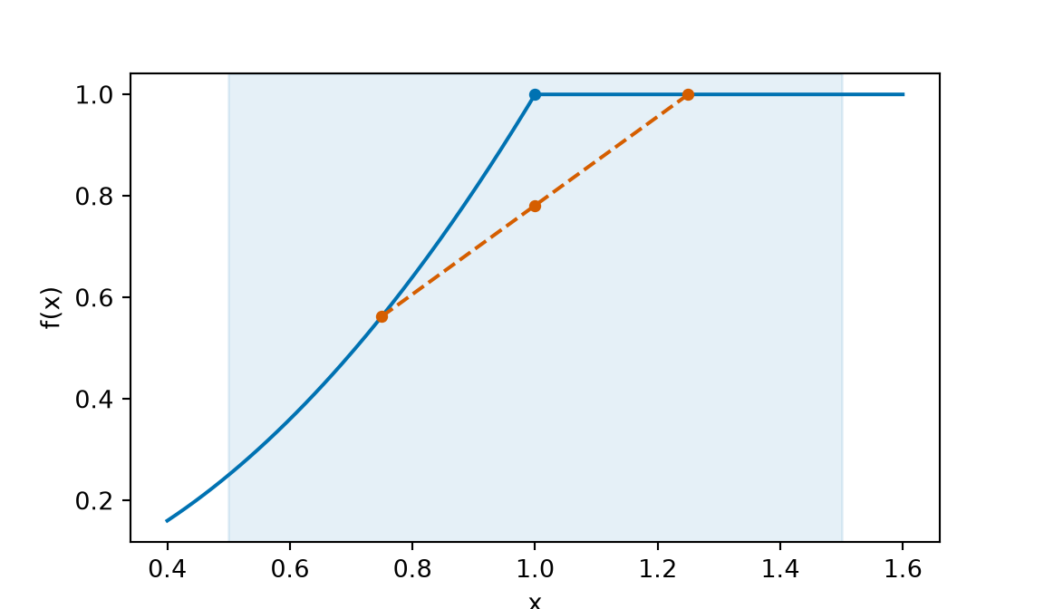
Example 8 (A function convex at one point and not at another) Let $f(x) = {\min\mathopen{}\left(x^2, 1\right)\mathclose{}}$, as in Example 7.

$f$ is convex at $0$: the open ball of radius $1$ around $0$ is $(-1, 1)$, a subset of $[-1, 1]$, and $f$ is convex on $[-1, 1]$ by Example 7, so the defining inequality holds for all $x, y \in (-1, 1)$ as well.
$f$ is not convex at $1$. Take any $r > 0$, let $\varepsilon= \tfrac{1}{2} {\min\mathopen{}\left(r, 1\right)\mathclose{}}$, and take $x = 1 - \varepsilon$, $y = 1 + \varepsilon$ and $t = \tfrac{1}{2}$, so that $x$ and $y$ are in the open ball of radius $r$ around $1$ and $t x + (1 - t) y = 1$. Then $f(1) = 1$, while

\[ \begin{aligned} \tfrac{1}{2} f(1 - \varepsilon) + \tfrac{1}{2} f(1 + \varepsilon) &= \tfrac{1}{2} (1 - \varepsilon)^2 + \tfrac{1}{2} \cdot 1 && \text{(} 0 < 1 - \varepsilon< 1 < 1 + \varepsilon\text{)} \\ &< \tfrac{1}{2} + \tfrac{1}{2} && \text{(} (1 - \varepsilon)^2 < 1 \text{)} \\ &= 1, && \text{(add)} \end{aligned} \]

so the defining inequality fails on every open ball around $1$.

In Figure 5, the chord from $1 - \varepsilon$ to $1 + \varepsilon$ passes below the graph at $1$.

Show code

ca_x_ca <- seq(0.4, 1.6, length.out = 241)
ca_square_ca <- ca_x_ca^2
ca_f_ca <- pmin(ca_square_ca, 1)
ca_graph_ca <- tibble::tibble(x = ca_x_ca, f = ca_f_ca)
ca_ends_ca <- c(0.75, 1.25)
ca_end_squares_ca <- ca_ends_ca^2
ca_end_f_ca <- pmin(ca_end_squares_ca, 1)
ca_chord_ca <- tibble::tibble(x = ca_ends_ca, f = ca_end_f_ca)
ca_chord_mid_ca <- mean(ca_end_f_ca)
ca_mid_x_ca <- c(1, 1)
ca_mid_f_ca <- c(ca_chord_mid_ca, 1)
ca_mid_ca <- tibble::tibble(x = ca_mid_x_ca, f = ca_mid_f_ca)
ca_mid_cols_ca <- c("#D55E00", "#0072B2")
ca_graph_ca |>
  ggplot2::ggplot() +
  ggplot2::aes(x = x, y = f) +
  ggplot2::annotate(
    "rect",
    xmin = 0.5, xmax = 1.5, ymin = -Inf, ymax = Inf,
    fill = "#0072B2", alpha = 0.1
  ) +
  ggplot2::geom_line(colour = "#0072B2") +
  ggplot2::geom_line(
    data = ca_chord_ca, colour = "#D55E00", linetype = "dashed"
  ) +
  ggplot2::geom_point(data = ca_chord_ca, colour = "#D55E00", size = 2) +
  ggplot2::geom_point(data = ca_mid_ca, colour = ca_mid_cols_ca, size = 2) +
  ggplot2::labs(x = "x", y = "f(x)") +
  ggplot2::theme_minimal()

Show code

import matplotlib.pyplot as plt
import numpy as np

ca_x_py = np.linspace(0.4, 1.6, 241)
ca_f_py = np.minimum(ca_x_py**2, 1)
ca_ends_py = np.array([0.75, 1.25])
ca_end_f_py = np.minimum(ca_ends_py**2, 1)
fig, ax = plt.subplots(figsize=(6, 3.5))
ax.axvspan(0.5, 1.5, color="#0072B2", alpha=0.1)
ax.plot(ca_x_py, ca_f_py, color="#0072B2")
ax.plot(ca_ends_py, ca_end_f_py, "--o", color="#D55E00", markersize=4)
ax.plot([1], [ca_end_f_py.mean()], "o", color="#D55E00", markersize=4)
ax.plot([1], [1], "o", color="#0072B2", markersize=4)
ax.set_xlabel("x")
ax.set_ylabel("f(x)")
plt.show();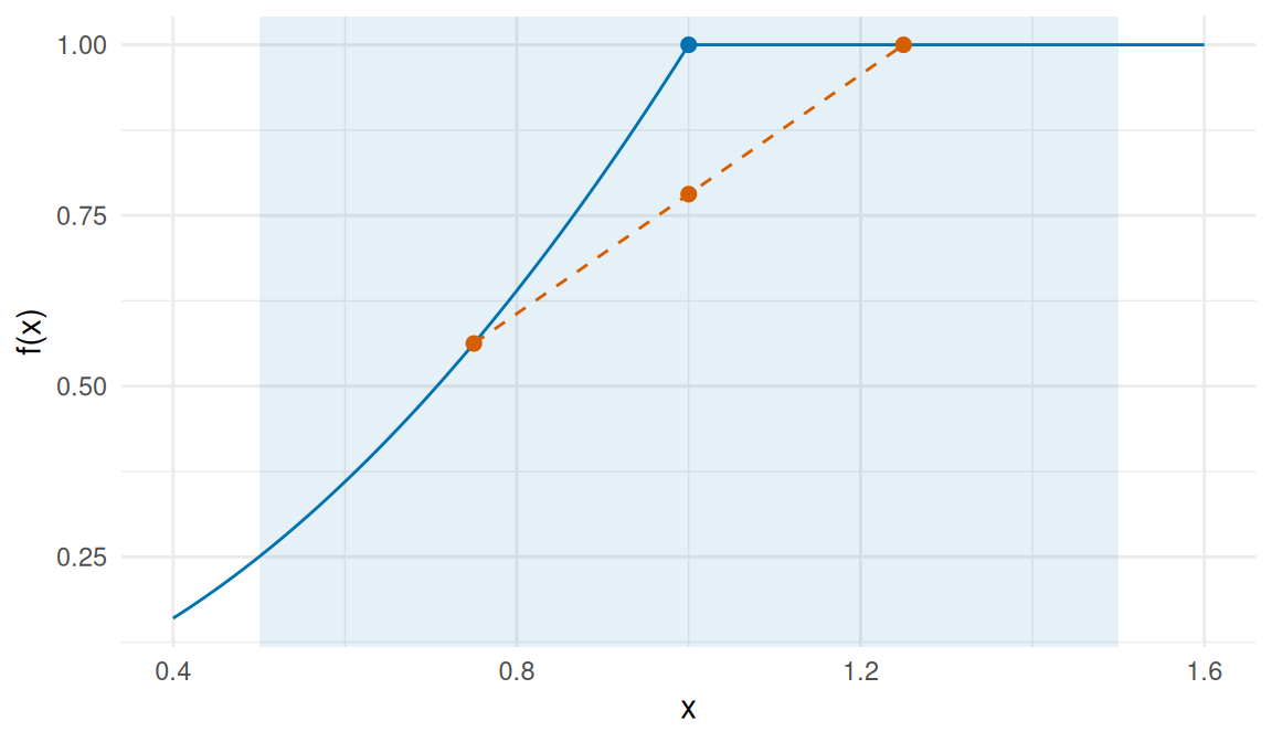

The graph of f(x) = min(x^2, 1) for x from 0.4 to 1.6: rising as x^2 up to x = 1, then flat at height 1. The open ball of radius 0.5 around 1, the interval from 0.5 to 1.5, is shaded. A dashed vermilion chord joins (0.75, 0.5625) and (1.25, 1) and passes through (1, 0.78125), below the graph's value 1 at x = 1. — Figure 5: The graph of $f(x) = {\min\mathopen{}\left(x^2, 1\right)\mathclose{}}$ near $1$, from Example 8, with $r = \tfrac{1}{2}$ and $\varepsilon= \tfrac{1}{4}$. The dashed chord from $\tfrac{3}{4}$ to $\tfrac{5}{4}$ stays inside the shaded open ball of radius $r$ around $1$, and is at $\tfrac{25}{32}$ above $x = 1$, below $f(1) = 1$.

Theorem 3 (The maximum of convex functions is convex)

Theorem 3 (The maximum of convex functions is convex) If $f_1$ and $f_2$ are convex functions on $\mathbb{R}^p$, then $f(\mathord{\smash[b]{\underset{\raise.3ex\hbox{$\scriptstyle\sim$}}{x}}\vphantom{x}}) \stackrel{\text{def}}{=}\max\mathopen{}\left\{f_1(\mathord{\smash[b]{\underset{\raise.3ex\hbox{$\scriptstyle\sim$}}{x}}\vphantom{x}}), f_2(\mathord{\smash[b]{\underset{\raise.3ex\hbox{$\scriptstyle\sim$}}{x}}\vphantom{x}})\right\}\mathclose{}$ is convex.

Proof

\[ \begin{aligned} f_i(t \mathord{\smash[b]{\underset{\raise.3ex\hbox{$\scriptstyle\sim$}}{x}}\vphantom{x}}+ (1 - t) \mathord{\smash[b]{\underset{\raise.3ex\hbox{$\scriptstyle\sim$}}{y}}\vphantom{y}}) &\le t f_i(\mathord{\smash[b]{\underset{\raise.3ex\hbox{$\scriptstyle\sim$}}{x}}\vphantom{x}}) + (1 - t) f_i(\mathord{\smash[b]{\underset{\raise.3ex\hbox{$\scriptstyle\sim$}}{y}}\vphantom{y}}) && \text{(} f_i \text{ is convex)} \\ &\le t f(\mathord{\smash[b]{\underset{\raise.3ex\hbox{$\scriptstyle\sim$}}{x}}\vphantom{x}}) + (1 - t) f(\mathord{\smash[b]{\underset{\raise.3ex\hbox{$\scriptstyle\sim$}}{y}}\vphantom{y}}). && \text{(} f_i \le f \text{, and } t, 1 - t \ge 0 \text{)} \end{aligned} \]

Both $f_1$ and $f_2$ at $t \mathord{\smash[b]{\underset{\raise.3ex\hbox{$\scriptstyle\sim$}}{x}}\vphantom{x}}+ (1 - t) \mathord{\smash[b]{\underset{\raise.3ex\hbox{$\scriptstyle\sim$}}{y}}\vphantom{y}}$ are at most $t f(\mathord{\smash[b]{\underset{\raise.3ex\hbox{$\scriptstyle\sim$}}{x}}\vphantom{x}}) + (1 - t) f(\mathord{\smash[b]{\underset{\raise.3ex\hbox{$\scriptstyle\sim$}}{y}}\vphantom{y}})$, so their maximum $f(t \mathord{\smash[b]{\underset{\raise.3ex\hbox{$\scriptstyle\sim$}}{x}}\vphantom{x}}+ (1 - t) \mathord{\smash[b]{\underset{\raise.3ex\hbox{$\scriptstyle\sim$}}{y}}\vphantom{y}})$ is too.

Example 9 (A maximum is convex; a minimum need not be)

Example 9 (A maximum is convex; a minimum need not be)

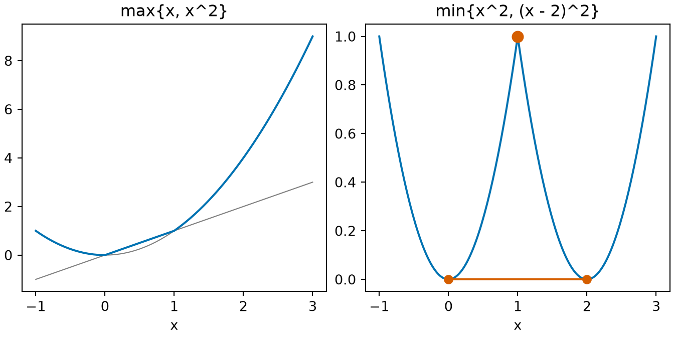
$f_1(x) = x$ is convex, by the computation for $2x + 1$ in Example 6 with $2$ and $1$ replaced by $1$ and $0$, and $f_2(x) = x^2$ is convex by the same example, so $\max\mathopen{}\left\{x, x^2\right\}\mathclose{}$ is convex by Theorem 3.
The minimum of two convex functions need not be convex: $g(x) = \min\mathopen{}\left\{x^2, (x - 2)^2\right\}\mathclose{}$ has

\[ \begin{aligned} g(0) &= g(2) \\ &= 0, \end{aligned} \]

but at the midpoint

\[ \begin{aligned} g(1) &= \min\mathopen{}\left\{1, 1\right\}\mathclose{} \\ &= 1 \\ &> \tfrac{1}{2} g(0) + \tfrac{1}{2} g(2) \\ &= 0. \end{aligned} \]

Show code

cm_x_fm <- seq(-1, 3, length.out = 201)
cm_levels_fm <- c("max{x, x^2}", "min{x^2, (x - 2)^2}")
cm_max_value_fm <- pmax(cm_x_fm, cm_x_fm^2)
cm_min_value_fm <- pmin(cm_x_fm^2, (cm_x_fm - 2)^2)
cm_max_fm <- tibble::tibble(
  x = cm_x_fm, value = cm_max_value_fm, panel = cm_levels_fm[1]
)
cm_min_fm <- tibble::tibble(
  x = cm_x_fm, value = cm_min_value_fm, panel = cm_levels_fm[2]
)
cm_main_fm <- dplyr::bind_rows(cm_max_fm, cm_min_fm)
cm_main_fm$panel <- factor(cm_main_fm$panel, levels = cm_levels_fm)
cm_square_value_fm <- cm_x_fm^2
cm_line_fm <- tibble::tibble(
  x = cm_x_fm, value = cm_x_fm, panel = cm_levels_fm[1], part = "x"
)
cm_square_fm <- tibble::tibble(
  x = cm_x_fm, value = cm_square_value_fm, panel = cm_levels_fm[1],
  part = "x^2"
)
cm_parts_fm <- dplyr::bind_rows(cm_line_fm, cm_square_fm)
cm_parts_fm$panel <- factor(cm_parts_fm$panel, levels = cm_levels_fm)
cm_chord_fm <- tibble::tibble(
  x = 0, xend = 2, value = 0, panel = cm_levels_fm[2]
)
cm_chord_fm$panel <- factor(cm_chord_fm$panel, levels = cm_levels_fm)
cm_mid_fm <- tibble::tibble(x = 1, value = 1, panel = cm_levels_fm[2])
cm_mid_fm$panel <- factor(cm_mid_fm$panel, levels = cm_levels_fm)
cm_aes_fm <- ggplot2::aes(x, value)
cm_parts_aes_fm <- ggplot2::aes(group = part)
cm_chord_aes_fm <- ggplot2::aes(xend = xend, yend = value)
ggplot2::ggplot(cm_main_fm, cm_aes_fm) +
  ggplot2::geom_line(
    data = cm_parts_fm, mapping = cm_parts_aes_fm,
    colour = "grey60", linewidth = 0.4
  ) +
  ggplot2::geom_line(colour = "#0072B2") +
  ggplot2::geom_segment(
    data = cm_chord_fm, mapping = cm_chord_aes_fm, colour = "#D55E00"
  ) +
  ggplot2::geom_point(data = cm_mid_fm, colour = "#D55E00", size = 3) +
  ggplot2::facet_wrap(~panel, scales = "free_y") +
  ggplot2::labs(x = "x", y = NULL)

Show code

import matplotlib.pyplot as plt
import numpy as np

cm_x_fm = np.linspace(-1, 3, 201)
fig, axes = plt.subplots(1, 2, figsize=(7, 3.5), layout="constrained")
axes[0].plot(cm_x_fm, cm_x_fm, color="grey", linewidth=0.8)
axes[0].plot(cm_x_fm, cm_x_fm**2, color="grey", linewidth=0.8)
axes[0].plot(cm_x_fm, np.maximum(cm_x_fm, cm_x_fm**2), color="#0072B2")
axes[0].set_title("max{x, x^2}")
axes[1].plot(cm_x_fm, np.minimum(cm_x_fm**2, (cm_x_fm - 2)**2), color="#0072B2")
axes[1].plot([0, 2], [0, 0], "o-", color="#D55E00", markersize=6)
axes[1].plot(1, 1, "o", color="#D55E00", markersize=8)
axes[1].set_title("min{x^2, (x - 2)^2}")
for ax in axes:
    ax.set_xlabel("x")
plt.show()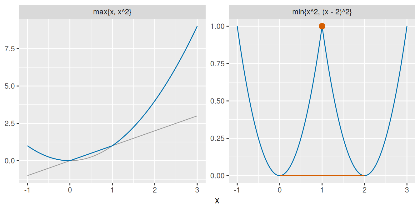

Two panels over x. Left: the lines x and x squared in thin grey and their pointwise maximum in blue, a curve that is convex. Right: the curve g of x, the smaller of x squared and x minus 2 squared, in blue, a double dip with a peak of 1 at x of 1. A vermilion segment along the x-axis joins the points (0, 0) and (2, 0) on the curve, and a vermilion circle at (1, 1) lies above that segment. — Figure 6: The functions of Example 9. The maximum of the two convex functions on the left is again one. The minimum on the right is not: $g(1) = 1$ is above $\tfrac{1}{2} g(0) + \tfrac{1}{2} g(2) = 0$, the height of the segment.

Definition 9 (Epigraph)

Definition 9 (Epigraph) The epigraph [4] of $f : \mathbb{R}^p \to \mathbb{R}$ is the set of points on or over its graph,

\[ \operatorname{epi} f \stackrel{\text{def}}{=}\mathopen{}\left\{(\mathord{\smash[b]{\underset{\raise.3ex\hbox{$\scriptstyle\sim$}}{x}}\vphantom{x}}, s) : \mathord{\smash[b]{\underset{\raise.3ex\hbox{$\scriptstyle\sim$}}{x}}\vphantom{x}}\in \mathbb{R}^p,\ s \in \mathbb{R},\ f(\mathord{\smash[b]{\underset{\raise.3ex\hbox{$\scriptstyle\sim$}}{x}}\vphantom{x}}) \le s\right\}\mathclose{}. \]

A pair $(\mathord{\smash[b]{\underset{\raise.3ex\hbox{$\scriptstyle\sim$}}{x}}\vphantom{x}}, s)$ is treated as the $(p + 1)$-vector with entries $x_1, \ldots, x_p, s$, so $\operatorname{epi} f \subseteq \mathbb{R}^{p+1}$, and sums and multiples of pairs are taken entry by entry.

Example 10 (The epigraph of $x^2$)

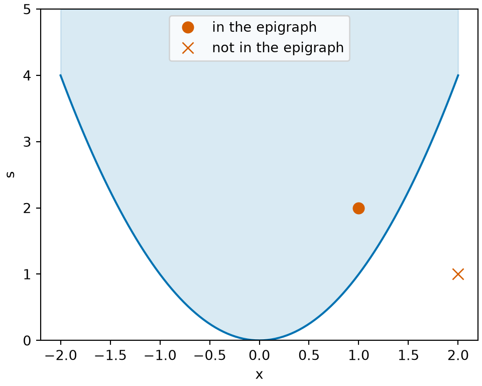
Example 10 (The epigraph of $x^2$) For $f(x) = x^2$, $\operatorname{epi} f = \mathopen{}\left\{(x, s) : x^2 \le s\right\}\mathclose{}$, the points $(x, s)$ on the parabola $s = x^2$ or on the side of it where $s$ is larger. $(1, 2)$ is in it, since $1^2 \le 2$; $(2, 1)$ is not, since $2^2 > 1$.

Show code

ep_x_fe <- seq(-2, 2, length.out = 201)
ep_curve_fe <- tibble::tibble(x = ep_x_fe, s = ep_x_fe^2, top = 5)
ep_marks_x_fe <- c(1, 2)
ep_marks_s_fe <- c(2, 1)
ep_marks_kind_fe <- c("in the epigraph", "not in the epigraph")
ep_marks_fe <- tibble::tibble(
  x = ep_marks_x_fe, s = ep_marks_s_fe, kind = ep_marks_kind_fe
)
ep_aes_fe <- ggplot2::aes(x, s)
ep_ribbon_aes_fe <- ggplot2::aes(ymin = s, ymax = top)
ep_marks_aes_fe <- ggplot2::aes(shape = kind)
ep_shapes_fe <- c("in the epigraph" = 16, "not in the epigraph" = 4)
ggplot2::ggplot(ep_curve_fe, ep_aes_fe) +
  ggplot2::geom_ribbon(
    mapping = ep_ribbon_aes_fe, fill = "#0072B2", alpha = 0.15
  ) +
  ggplot2::geom_line(colour = "#0072B2") +
  ggplot2::geom_point(
    data = ep_marks_fe, mapping = ep_marks_aes_fe,
    colour = "#D55E00", size = 3
  ) +
  ggplot2::scale_shape_manual(values = ep_shapes_fe) +
  ggplot2::labs(x = "x", y = "s", shape = NULL)

Show code

import matplotlib.pyplot as plt
import numpy as np

ep_x_fe = np.linspace(-2, 2, 201)
fig, ax = plt.subplots(figsize=(5, 4), layout="constrained")
ax.fill_between(ep_x_fe, ep_x_fe**2, 5, color="#0072B2", alpha=0.15)
ax.plot(ep_x_fe, ep_x_fe**2, color="#0072B2")
ax.plot(1, 2, "o", color="#D55E00", markersize=8, label="in the epigraph")
ax.plot(2, 1, "x", color="#D55E00", markersize=8, label="not in the epigraph")
ax.set_ylim(0, 5)
#> (0.0, 5.0)
ax.set_xlabel("x")
ax.set_ylabel("s")
ax.legend(loc="upper center")
plt.show()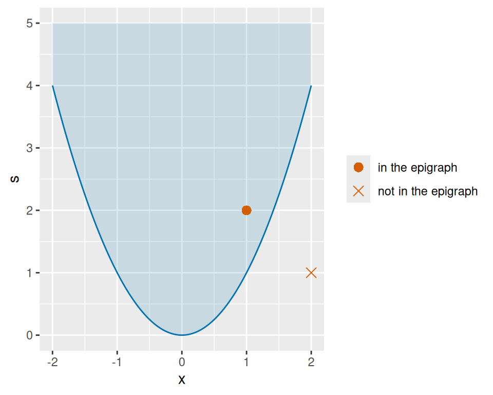

Plot of the parabola s equals x squared for x from -2 to 2. The region on and above the parabola is shaded light blue. A vermilion filled circle at (1, 2) lies in the shaded region, and a vermilion cross at (2, 1) lies below the parabola, outside it. — Figure 7: The epigraph of $f(x) = x^2$ (Example 10): the shaded points on or above the parabola. $(1, 2)$ is in it, and $(2, 1)$ is not.

Theorem 4 (Convexity through the epigraph)

Theorem 4 (Convexity through the epigraph) $f : \mathbb{R}^p \to \mathbb{R}$ is convex if and only if its epigraph (Definition 9) is convex (Definition 1).

Proof

Proof. If. Let $\mathord{\smash[b]{\underset{\raise.3ex\hbox{$\scriptstyle\sim$}}{x}}\vphantom{x}}, \mathord{\smash[b]{\underset{\raise.3ex\hbox{$\scriptstyle\sim$}}{y}}\vphantom{y}}\in \mathbb{R}^p$ and $t \in [0, 1]$. The points $(\mathord{\smash[b]{\underset{\raise.3ex\hbox{$\scriptstyle\sim$}}{x}}\vphantom{x}}, f(\mathord{\smash[b]{\underset{\raise.3ex\hbox{$\scriptstyle\sim$}}{x}}\vphantom{x}}))$ and $(\mathord{\smash[b]{\underset{\raise.3ex\hbox{$\scriptstyle\sim$}}{y}}\vphantom{y}}, f(\mathord{\smash[b]{\underset{\raise.3ex\hbox{$\scriptstyle\sim$}}{y}}\vphantom{y}}))$ are in $\operatorname{epi} f$, since $f(\mathord{\smash[b]{\underset{\raise.3ex\hbox{$\scriptstyle\sim$}}{x}}\vphantom{x}}) \le f(\mathord{\smash[b]{\underset{\raise.3ex\hbox{$\scriptstyle\sim$}}{x}}\vphantom{x}})$ and $f(\mathord{\smash[b]{\underset{\raise.3ex\hbox{$\scriptstyle\sim$}}{y}}\vphantom{y}}) \le f(\mathord{\smash[b]{\underset{\raise.3ex\hbox{$\scriptstyle\sim$}}{y}}\vphantom{y}})$. Since $\operatorname{epi} f$ is convex, it contains

\[ t\,(\mathord{\smash[b]{\underset{\raise.3ex\hbox{$\scriptstyle\sim$}}{x}}\vphantom{x}}, f(\mathord{\smash[b]{\underset{\raise.3ex\hbox{$\scriptstyle\sim$}}{x}}\vphantom{x}})) + (1 - t)\,(\mathord{\smash[b]{\underset{\raise.3ex\hbox{$\scriptstyle\sim$}}{y}}\vphantom{y}}, f(\mathord{\smash[b]{\underset{\raise.3ex\hbox{$\scriptstyle\sim$}}{y}}\vphantom{y}})) = \mathopen{}\left(t \mathord{\smash[b]{\underset{\raise.3ex\hbox{$\scriptstyle\sim$}}{x}}\vphantom{x}}+ (1 - t) \mathord{\smash[b]{\underset{\raise.3ex\hbox{$\scriptstyle\sim$}}{y}}\vphantom{y}},\ t f(\mathord{\smash[b]{\underset{\raise.3ex\hbox{$\scriptstyle\sim$}}{x}}\vphantom{x}}) + (1 - t) f(\mathord{\smash[b]{\underset{\raise.3ex\hbox{$\scriptstyle\sim$}}{y}}\vphantom{y}})\right)\mathclose{}, \]

and by Definition 9 that membership means $f(t \mathord{\smash[b]{\underset{\raise.3ex\hbox{$\scriptstyle\sim$}}{x}}\vphantom{x}}+ (1 - t) \mathord{\smash[b]{\underset{\raise.3ex\hbox{$\scriptstyle\sim$}}{y}}\vphantom{y}}) \le t f(\mathord{\smash[b]{\underset{\raise.3ex\hbox{$\scriptstyle\sim$}}{x}}\vphantom{x}}) + (1 - t) f(\mathord{\smash[b]{\underset{\raise.3ex\hbox{$\scriptstyle\sim$}}{y}}\vphantom{y}})$.

Only if. Let $(\mathord{\smash[b]{\underset{\raise.3ex\hbox{$\scriptstyle\sim$}}{x}}\vphantom{x}}, s)$ and $(\mathord{\smash[b]{\underset{\raise.3ex\hbox{$\scriptstyle\sim$}}{y}}\vphantom{y}}, u)$ be in $\operatorname{epi} f$, so $f(\mathord{\smash[b]{\underset{\raise.3ex\hbox{$\scriptstyle\sim$}}{x}}\vphantom{x}}) \le s$ and $f(\mathord{\smash[b]{\underset{\raise.3ex\hbox{$\scriptstyle\sim$}}{y}}\vphantom{y}}) \le u$, and let $t \in [0, 1]$. Then

\[ \begin{aligned} f(t \mathord{\smash[b]{\underset{\raise.3ex\hbox{$\scriptstyle\sim$}}{x}}\vphantom{x}}+ (1 - t) \mathord{\smash[b]{\underset{\raise.3ex\hbox{$\scriptstyle\sim$}}{y}}\vphantom{y}}) &\le t f(\mathord{\smash[b]{\underset{\raise.3ex\hbox{$\scriptstyle\sim$}}{x}}\vphantom{x}}) + (1 - t) f(\mathord{\smash[b]{\underset{\raise.3ex\hbox{$\scriptstyle\sim$}}{y}}\vphantom{y}}) && \text{(} f \text{ is convex)} \\ &\le t s + (1 - t) u, && \text{(} f(\mathord{\smash[b]{\underset{\raise.3ex\hbox{$\scriptstyle\sim$}}{x}}\vphantom{x}}) \le s \text{, } f(\mathord{\smash[b]{\underset{\raise.3ex\hbox{$\scriptstyle\sim$}}{y}}\vphantom{y}}) \le u \text{, and } t, 1 - t \ge 0 \text{)} \end{aligned} \]

so $t\,(\mathord{\smash[b]{\underset{\raise.3ex\hbox{$\scriptstyle\sim$}}{x}}\vphantom{x}}, s) + (1 - t)\,(\mathord{\smash[b]{\underset{\raise.3ex\hbox{$\scriptstyle\sim$}}{y}}\vphantom{y}}, u) = (t \mathord{\smash[b]{\underset{\raise.3ex\hbox{$\scriptstyle\sim$}}{x}}\vphantom{x}}+ (1 - t) \mathord{\smash[b]{\underset{\raise.3ex\hbox{$\scriptstyle\sim$}}{y}}\vphantom{y}},\ t s + (1 - t) u)$ is in $\operatorname{epi} f$.

Example 11 (Two epigraphs)

Example 11 (Two epigraphs)

The epigraph of $f(x) = \mathopen{}\left|x\right|\mathclose{}$ is $\mathopen{}\left\{(x, s) : \mathopen{}\left|x\right|\mathclose{} \le s\right\}\mathclose{}$, a wedge. It is the intersection of the half-planes $\mathopen{}\left\{(x, s) : s - x \ge 0\right\}\mathclose{}$ and $\mathopen{}\left\{(x, s) : s + x \ge 0\right\}\mathclose{}$. Each half-plane is convex: if $s_1 - x_1 \ge 0$ and $s_2 - x_2 \ge 0$, then $(t s_1 + (1 - t) s_2) - (t x_1 + (1 - t) x_2) = t (s_1 - x_1) + (1 - t)(s_2 - x_2) \ge 0$, and the same with $+$ for the other. So the wedge is convex (Theorem 1), and $\mathopen{}\left|x\right|\mathclose{}$ is convex by Theorem 4.
The epigraph of $g(x) = -x^2$ is not convex: $(-1, -1)$ and $(1, -1)$ are in it, since $g(\pm 1) = -1$, but their midpoint $(0, -1)$ is not, since $g(0) = 0 > -1$. So $-x^2$ is not convex.

Definition 10 (Tangent plane)

Definition 10 (Tangent plane) Let $f : \mathbb{R}^p \to \mathbb{R}$ have a gradient at $\mathord{\smash[b]{\underset{\raise.3ex\hbox{$\scriptstyle\sim$}}{y}}\vphantom{y}}$. The tangent plane [5] to the graph of $f$ at $\mathord{\smash[b]{\underset{\raise.3ex\hbox{$\scriptstyle\sim$}}{y}}\vphantom{y}}$ is the graph of the function

\[ \mathord{\smash[b]{\underset{\raise.3ex\hbox{$\scriptstyle\sim$}}{x}}\vphantom{x}}\mapsto f(\mathord{\smash[b]{\underset{\raise.3ex\hbox{$\scriptstyle\sim$}}{y}}\vphantom{y}}) + {\mathopen{}\left(\frac{\partial}{\partial \mathord{\smash[b]{\underset{\raise.3ex\hbox{$\scriptstyle\sim$}}{x}}\vphantom{x}}} f(\mathord{\smash[b]{\underset{\raise.3ex\hbox{$\scriptstyle\sim$}}{y}}\vphantom{y}})\right)\mathclose{}}^{\top} (\mathord{\smash[b]{\underset{\raise.3ex\hbox{$\scriptstyle\sim$}}{x}}\vphantom{x}}- \mathord{\smash[b]{\underset{\raise.3ex\hbox{$\scriptstyle\sim$}}{y}}\vphantom{y}}), \]

which takes the value $f(\mathord{\smash[b]{\underset{\raise.3ex\hbox{$\scriptstyle\sim$}}{y}}\vphantom{y}})$ at $\mathord{\smash[b]{\underset{\raise.3ex\hbox{$\scriptstyle\sim$}}{x}}\vphantom{x}}= \mathord{\smash[b]{\underset{\raise.3ex\hbox{$\scriptstyle\sim$}}{y}}\vphantom{y}}$ and has the same gradient as $f$ there.

Example 12 (A tangent line and a tangent plane)

Example 12 (A tangent line and a tangent plane)

For $f(x) = x^2$ at $y = 1$, $f(1) = 1$ and $f'(1) = 2$, so the tangent line is

\[ \begin{aligned} s &= 1 + 2\,(x - 1) && \text{(substitute } f(1) \text{ and } f'(1) \text{)} \\ &= 1 + 2x - 2 && \text{(distribute)} \\ &= 2x - 1. && \text{(} 1 - 2 = -1 \text{)} \end{aligned} \]
For $f(\mathord{\smash[b]{\underset{\raise.3ex\hbox{$\scriptstyle\sim$}}{x}}\vphantom{x}}) = x_1^2 + x_2^2$ at $\mathord{\smash[b]{\underset{\raise.3ex\hbox{$\scriptstyle\sim$}}{y}}\vphantom{y}}= {(1, 1)}^{\top}$, $f(\mathord{\smash[b]{\underset{\raise.3ex\hbox{$\scriptstyle\sim$}}{y}}\vphantom{y}}) = 2$ and the gradient is $\nabla f(\mathord{\smash[b]{\underset{\raise.3ex\hbox{$\scriptstyle\sim$}}{y}}\vphantom{y}}) = {(2 y_1,\ 2 y_2)}^{\top} = {(2, 2)}^{\top}$, so the tangent plane is

\[ \begin{aligned} s &= 2 + 2\,(x_1 - 1) + 2\,(x_2 - 1) && \text{(substitute } f(\mathord{\smash[b]{\underset{\raise.3ex\hbox{$\scriptstyle\sim$}}{y}}\vphantom{y}}) \text{ and the gradient)} \\ &= 2 + 2 x_1 - 2 + 2 x_2 - 2 && \text{(distribute)} \\ &= 2 x_1 + 2 x_2 - 2. && \text{(} 2 - 2 - 2 = -2 \text{)} \end{aligned} \]

Figure 8 shows the tangent plane of the second bullet.

Show code

tp_x_tp <- seq(-1, 3, length.out = 41)
tp_square_tp <- tp_x_tp^2
tp_double_tp <- 2 * tp_x_tp
tp_bowl_tp <- outer(tp_square_tp, tp_square_tp, "+")
tp_sum_tp <- outer(tp_double_tp, tp_double_tp, "+")
tp_plane_tp <- tp_sum_tp - 2
tp_point_tp <- tibble::tibble(x1 = 1, x2 = 1, z = 2)
tp_black_tp <- list(color = "#000000", size = 5)
tp_stops_tp <- c(0, 1)
tp_blue_cols_tp <- c("#CCE0F0", "#0072B2")
tp_red_cols_tp <- c("#D55E00", "#D55E00")
tp_blue_tp <- list(tp_stops_tp, tp_blue_cols_tp)
tp_red_tp <- list(tp_stops_tp, tp_red_cols_tp)
tp_eye_tp <- list(x = 1.6, y = -1.6, z = 0.9)
tp_camera_tp <- list(eye = tp_eye_tp)
tp_xaxis_tp <- list(title = "x1")
tp_yaxis_tp <- list(title = "x2")
tp_zaxis_tp <- list(title = "f(x)")
tp_scene_tp <- list(
  xaxis = tp_xaxis_tp,
  yaxis = tp_yaxis_tp,
  zaxis = tp_zaxis_tp,
  camera = tp_camera_tp
)
tp_legend_tp <- list(orientation = "h")
plotly::plot_ly() |>
  plotly::add_surface(
    x = tp_x_tp,
    y = tp_x_tp,
    z = tp_bowl_tp,
    colorscale = tp_blue_tp,
    showscale = FALSE,
    opacity = 0.8
  ) |>
  plotly::add_surface(
    x = tp_x_tp,
    y = tp_x_tp,
    z = tp_plane_tp,
    colorscale = tp_red_tp,
    showscale = FALSE,
    opacity = 0.5
  ) |>
  plotly::add_trace(
    data = tp_point_tp,
    x = ~x1,
    y = ~x2,
    z = ~z,
    type = "scatter3d",
    mode = "markers",
    marker = tp_black_tp,
    name = "point of tangency"
  ) |>
  plotly::layout(scene = tp_scene_tp, legend = tp_legend_tp)

Show code

import matplotlib.pyplot as plt
import numpy as np

tp_x1_py, tp_x2_py = np.meshgrid(np.linspace(-1, 3, 41),
                                 np.linspace(-1, 3, 41))
tp_bowl_py = tp_x1_py**2 + tp_x2_py**2
tp_plane_py = 2 * tp_x1_py + 2 * tp_x2_py - 2
fig = plt.figure(figsize=(6, 4.5))
ax = fig.add_subplot(projection="3d")
ax.plot_surface(tp_x1_py, tp_x2_py, tp_bowl_py, color="#0072B2", alpha=0.6)
ax.plot_surface(tp_x1_py, tp_x2_py, tp_plane_py, color="#D55E00", alpha=0.4)
ax.scatter([1], [1], [2], color="black", label="point of tangency")
ax.set_xlabel("x1")
ax.set_ylabel("x2")
ax.set_zlabel("f(x)")
ax.legend(loc="upper right")
plt.show();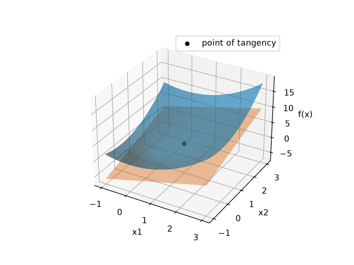

Surface plot of f(x) = x1^2 + x2^2 for x1 and x2 from -1 to 3, a bowl with its lowest point at the origin. A flat vermilion plane, the tangent plane 2 x1 + 2 x2 - 2, touches the bowl from below at the point (1, 1, 2), which is marked with a black point. — Figure 8: The tangent plane (vermilion) of the bowl $f(\mathord{\smash[b]{\underset{\raise.3ex\hbox{$\scriptstyle\sim$}}{x}}\vphantom{x}}) = x_1^2 + x_2^2$ of Example 12 touches it at ${(1, 1)}^{\top}$ and lies below it.

Remark 1 (The tangent plane in one variable)

Remark 1 (The tangent plane in one variable). For $p = 1$ the tangent plane is the tangent line $s = f(y) + f'(y)\,(x - y)$, the line through $(y, f(y))$ with slope $f'(y)$.

Theorem 5 (First-order characterization of convexity)

Theorem 5 (First-order characterization of convexity) Let $f : \mathbb{R}^p \to \mathbb{R}$ have first partial derivatives that are continuous on $\mathbb{R}^p$. Then $f$ is convex if and only if

\[ f(\mathord{\smash[b]{\underset{\raise.3ex\hbox{$\scriptstyle\sim$}}{x}}\vphantom{x}}) \ge f(\mathord{\smash[b]{\underset{\raise.3ex\hbox{$\scriptstyle\sim$}}{y}}\vphantom{y}}) + {\mathopen{}\left(\frac{\partial}{\partial \mathord{\smash[b]{\underset{\raise.3ex\hbox{$\scriptstyle\sim$}}{x}}\vphantom{x}}} f(\mathord{\smash[b]{\underset{\raise.3ex\hbox{$\scriptstyle\sim$}}{y}}\vphantom{y}})\right)\mathclose{}}^{\top} (\mathord{\smash[b]{\underset{\raise.3ex\hbox{$\scriptstyle\sim$}}{x}}\vphantom{x}}- \mathord{\smash[b]{\underset{\raise.3ex\hbox{$\scriptstyle\sim$}}{y}}\vphantom{y}}) \qquad \text{for all } \mathord{\smash[b]{\underset{\raise.3ex\hbox{$\scriptstyle\sim$}}{x}}\vphantom{x}}, \mathord{\smash[b]{\underset{\raise.3ex\hbox{$\scriptstyle\sim$}}{y}}\vphantom{y}}\in \mathbb{R}^p: \tag{1}\]

every tangent plane (Definition 10) lies on or under the graph. If the inequality is strict whenever $\mathord{\smash[b]{\underset{\raise.3ex\hbox{$\scriptstyle\sim$}}{x}}\vphantom{x}}\ne \mathord{\smash[b]{\underset{\raise.3ex\hbox{$\scriptstyle\sim$}}{y}}\vphantom{y}}$, then $f$ is strictly convex (Definition 4).

Proof

Proof. Only if. Let $\mathord{\smash[b]{\underset{\raise.3ex\hbox{$\scriptstyle\sim$}}{x}}\vphantom{x}}, \mathord{\smash[b]{\underset{\raise.3ex\hbox{$\scriptstyle\sim$}}{y}}\vphantom{y}}\in \mathbb{R}^p$, let $\mathord{\smash[b]{\underset{\raise.3ex\hbox{$\scriptstyle\sim$}}{d}}\vphantom{d}} \stackrel{\text{def}}{=}\mathord{\smash[b]{\underset{\raise.3ex\hbox{$\scriptstyle\sim$}}{x}}\vphantom{x}}- \mathord{\smash[b]{\underset{\raise.3ex\hbox{$\scriptstyle\sim$}}{y}}\vphantom{y}}$, and let $g(t) \stackrel{\text{def}}{=}f(\mathord{\smash[b]{\underset{\raise.3ex\hbox{$\scriptstyle\sim$}}{y}}\vphantom{y}}+ t \mathord{\smash[b]{\underset{\raise.3ex\hbox{$\scriptstyle\sim$}}{d}}\vphantom{d}})$. The inner function $t \mapsto \mathord{\smash[b]{\underset{\raise.3ex\hbox{$\scriptstyle\sim$}}{y}}\vphantom{y}}+ t \mathord{\smash[b]{\underset{\raise.3ex\hbox{$\scriptstyle\sim$}}{d}}\vphantom{d}}$ has derivative ${\mathord{\smash[b]{\underset{\raise.3ex\hbox{$\scriptstyle\sim$}}{d}}\vphantom{d}}}^{\top}$, so the vector chain rule gives

\[ \begin{aligned} g'(0) &= {\mathord{\smash[b]{\underset{\raise.3ex\hbox{$\scriptstyle\sim$}}{d}}\vphantom{d}}}^{\top}\,\frac{\partial}{\partial \mathord{\smash[b]{\underset{\raise.3ex\hbox{$\scriptstyle\sim$}}{x}}\vphantom{x}}} f(\mathord{\smash[b]{\underset{\raise.3ex\hbox{$\scriptstyle\sim$}}{y}}\vphantom{y}}) && \text{(vector chain rule)} \\ &= {\mathopen{}\left(\frac{\partial}{\partial \mathord{\smash[b]{\underset{\raise.3ex\hbox{$\scriptstyle\sim$}}{x}}\vphantom{x}}} f(\mathord{\smash[b]{\underset{\raise.3ex\hbox{$\scriptstyle\sim$}}{y}}\vphantom{y}})\right)\mathclose{}}^{\top} \mathord{\smash[b]{\underset{\raise.3ex\hbox{$\scriptstyle\sim$}}{d}}\vphantom{d}}. && \text{(a } 1 \times 1 \text{ matrix equals its transpose)} \end{aligned} \]

For $t \in (0, 1]$, $\mathord{\smash[b]{\underset{\raise.3ex\hbox{$\scriptstyle\sim$}}{y}}\vphantom{y}}+ t \mathord{\smash[b]{\underset{\raise.3ex\hbox{$\scriptstyle\sim$}}{d}}\vphantom{d}} = t \mathord{\smash[b]{\underset{\raise.3ex\hbox{$\scriptstyle\sim$}}{x}}\vphantom{x}}+ (1 - t) \mathord{\smash[b]{\underset{\raise.3ex\hbox{$\scriptstyle\sim$}}{y}}\vphantom{y}}$, so

\[ \begin{aligned} g(t) - g(0) &= f(t \mathord{\smash[b]{\underset{\raise.3ex\hbox{$\scriptstyle\sim$}}{x}}\vphantom{x}}+ (1 - t) \mathord{\smash[b]{\underset{\raise.3ex\hbox{$\scriptstyle\sim$}}{y}}\vphantom{y}}) - f(\mathord{\smash[b]{\underset{\raise.3ex\hbox{$\scriptstyle\sim$}}{y}}\vphantom{y}}) && \text{(definition of } g \text{)} \\ &\le t f(\mathord{\smash[b]{\underset{\raise.3ex\hbox{$\scriptstyle\sim$}}{x}}\vphantom{x}}) + (1 - t) f(\mathord{\smash[b]{\underset{\raise.3ex\hbox{$\scriptstyle\sim$}}{y}}\vphantom{y}}) - f(\mathord{\smash[b]{\underset{\raise.3ex\hbox{$\scriptstyle\sim$}}{y}}\vphantom{y}}) && \text{(} f \text{ is convex)} \\ &= t\,(f(\mathord{\smash[b]{\underset{\raise.3ex\hbox{$\scriptstyle\sim$}}{x}}\vphantom{x}}) - f(\mathord{\smash[b]{\underset{\raise.3ex\hbox{$\scriptstyle\sim$}}{y}}\vphantom{y}})), && \text{(collect terms)} \end{aligned} \]

and dividing by $t > 0$, $\dfrac{g(t) - g(0)}{t} \le f(\mathord{\smash[b]{\underset{\raise.3ex\hbox{$\scriptstyle\sim$}}{x}}\vphantom{x}}) - f(\mathord{\smash[b]{\underset{\raise.3ex\hbox{$\scriptstyle\sim$}}{y}}\vphantom{y}})$. As $t \to 0$ from the right, the left side tends to $g'(0)$ ($g$ is differentiable at $0$, so the one-sided limit equals the two-sided derivative), and a limit of numbers that are all at most $f(\mathord{\smash[b]{\underset{\raise.3ex\hbox{$\scriptstyle\sim$}}{x}}\vphantom{x}}) - f(\mathord{\smash[b]{\underset{\raise.3ex\hbox{$\scriptstyle\sim$}}{y}}\vphantom{y}})$ is at most $f(\mathord{\smash[b]{\underset{\raise.3ex\hbox{$\scriptstyle\sim$}}{x}}\vphantom{x}}) - f(\mathord{\smash[b]{\underset{\raise.3ex\hbox{$\scriptstyle\sim$}}{y}}\vphantom{y}})$. So ${\mathopen{}\left(\frac{\partial}{\partial \mathord{\smash[b]{\underset{\raise.3ex\hbox{$\scriptstyle\sim$}}{x}}\vphantom{x}}} f(\mathord{\smash[b]{\underset{\raise.3ex\hbox{$\scriptstyle\sim$}}{y}}\vphantom{y}})\right)\mathclose{}}^{\top} (\mathord{\smash[b]{\underset{\raise.3ex\hbox{$\scriptstyle\sim$}}{x}}\vphantom{x}}- \mathord{\smash[b]{\underset{\raise.3ex\hbox{$\scriptstyle\sim$}}{y}}\vphantom{y}}) \le f(\mathord{\smash[b]{\underset{\raise.3ex\hbox{$\scriptstyle\sim$}}{x}}\vphantom{x}}) - f(\mathord{\smash[b]{\underset{\raise.3ex\hbox{$\scriptstyle\sim$}}{y}}\vphantom{y}})$, which rearranges to Equation 1.

If. Let $\mathord{\smash[b]{\underset{\raise.3ex\hbox{$\scriptstyle\sim$}}{x}}\vphantom{x}}, \mathord{\smash[b]{\underset{\raise.3ex\hbox{$\scriptstyle\sim$}}{y}}\vphantom{y}}\in \mathbb{R}^p$, $t \in [0, 1]$, $\mathord{\smash[b]{\underset{\raise.3ex\hbox{$\scriptstyle\sim$}}{z}}\vphantom{z}} \stackrel{\text{def}}{=}t \mathord{\smash[b]{\underset{\raise.3ex\hbox{$\scriptstyle\sim$}}{x}}\vphantom{x}}+ (1 - t) \mathord{\smash[b]{\underset{\raise.3ex\hbox{$\scriptstyle\sim$}}{y}}\vphantom{y}}$, and $\mathord{\smash[b]{\underset{\raise.3ex\hbox{$\scriptstyle\sim$}}{g}}\vphantom{g}} \stackrel{\text{def}}{=}\frac{\partial}{\partial \mathord{\smash[b]{\underset{\raise.3ex\hbox{$\scriptstyle\sim$}}{x}}\vphantom{x}}} f(\mathord{\smash[b]{\underset{\raise.3ex\hbox{$\scriptstyle\sim$}}{z}}\vphantom{z}})$. Applying Equation 1 at the point $\mathord{\smash[b]{\underset{\raise.3ex\hbox{$\scriptstyle\sim$}}{z}}\vphantom{z}}$, once toward $\mathord{\smash[b]{\underset{\raise.3ex\hbox{$\scriptstyle\sim$}}{x}}\vphantom{x}}$ and once toward $\mathord{\smash[b]{\underset{\raise.3ex\hbox{$\scriptstyle\sim$}}{y}}\vphantom{y}}$,

\[ f(\mathord{\smash[b]{\underset{\raise.3ex\hbox{$\scriptstyle\sim$}}{x}}\vphantom{x}}) \ge f(\mathord{\smash[b]{\underset{\raise.3ex\hbox{$\scriptstyle\sim$}}{z}}\vphantom{z}}) + {\mathord{\smash[b]{\underset{\raise.3ex\hbox{$\scriptstyle\sim$}}{g}}\vphantom{g}}}^{\top} (\mathord{\smash[b]{\underset{\raise.3ex\hbox{$\scriptstyle\sim$}}{x}}\vphantom{x}}- \mathord{\smash[b]{\underset{\raise.3ex\hbox{$\scriptstyle\sim$}}{z}}\vphantom{z}}), \qquad f(\mathord{\smash[b]{\underset{\raise.3ex\hbox{$\scriptstyle\sim$}}{y}}\vphantom{y}}) \ge f(\mathord{\smash[b]{\underset{\raise.3ex\hbox{$\scriptstyle\sim$}}{z}}\vphantom{z}}) + {\mathord{\smash[b]{\underset{\raise.3ex\hbox{$\scriptstyle\sim$}}{g}}\vphantom{g}}}^{\top} (\mathord{\smash[b]{\underset{\raise.3ex\hbox{$\scriptstyle\sim$}}{y}}\vphantom{y}}- \mathord{\smash[b]{\underset{\raise.3ex\hbox{$\scriptstyle\sim$}}{z}}\vphantom{z}}). \]

Multiplying the first by $t \ge 0$ and the second by $1 - t \ge 0$ and adding,

\[ \begin{aligned} t f(\mathord{\smash[b]{\underset{\raise.3ex\hbox{$\scriptstyle\sim$}}{x}}\vphantom{x}}) + (1 - t) f(\mathord{\smash[b]{\underset{\raise.3ex\hbox{$\scriptstyle\sim$}}{y}}\vphantom{y}}) &\ge t \mathopen{}\left(f(\mathord{\smash[b]{\underset{\raise.3ex\hbox{$\scriptstyle\sim$}}{z}}\vphantom{z}}) + {\mathord{\smash[b]{\underset{\raise.3ex\hbox{$\scriptstyle\sim$}}{g}}\vphantom{g}}}^{\top} (\mathord{\smash[b]{\underset{\raise.3ex\hbox{$\scriptstyle\sim$}}{x}}\vphantom{x}}- \mathord{\smash[b]{\underset{\raise.3ex\hbox{$\scriptstyle\sim$}}{z}}\vphantom{z}})\right)\mathclose{} + (1 - t) \mathopen{}\left(f(\mathord{\smash[b]{\underset{\raise.3ex\hbox{$\scriptstyle\sim$}}{z}}\vphantom{z}}) + {\mathord{\smash[b]{\underset{\raise.3ex\hbox{$\scriptstyle\sim$}}{g}}\vphantom{g}}}^{\top} (\mathord{\smash[b]{\underset{\raise.3ex\hbox{$\scriptstyle\sim$}}{y}}\vphantom{y}}- \mathord{\smash[b]{\underset{\raise.3ex\hbox{$\scriptstyle\sim$}}{z}}\vphantom{z}})\right)\mathclose{} && \text{(multiply by } t, 1 - t \ge 0 \text{ and add)} \\ &= (t + (1 - t))\,f(\mathord{\smash[b]{\underset{\raise.3ex\hbox{$\scriptstyle\sim$}}{z}}\vphantom{z}}) + t\,{\mathord{\smash[b]{\underset{\raise.3ex\hbox{$\scriptstyle\sim$}}{g}}\vphantom{g}}}^{\top} (\mathord{\smash[b]{\underset{\raise.3ex\hbox{$\scriptstyle\sim$}}{x}}\vphantom{x}}- \mathord{\smash[b]{\underset{\raise.3ex\hbox{$\scriptstyle\sim$}}{z}}\vphantom{z}}) + (1 - t)\,{\mathord{\smash[b]{\underset{\raise.3ex\hbox{$\scriptstyle\sim$}}{g}}\vphantom{g}}}^{\top} (\mathord{\smash[b]{\underset{\raise.3ex\hbox{$\scriptstyle\sim$}}{y}}\vphantom{y}}- \mathord{\smash[b]{\underset{\raise.3ex\hbox{$\scriptstyle\sim$}}{z}}\vphantom{z}}) && \text{(distribute } t \text{ and } 1 - t \text{)} \\ &= f(\mathord{\smash[b]{\underset{\raise.3ex\hbox{$\scriptstyle\sim$}}{z}}\vphantom{z}}) + t\,{\mathord{\smash[b]{\underset{\raise.3ex\hbox{$\scriptstyle\sim$}}{g}}\vphantom{g}}}^{\top} (\mathord{\smash[b]{\underset{\raise.3ex\hbox{$\scriptstyle\sim$}}{x}}\vphantom{x}}- \mathord{\smash[b]{\underset{\raise.3ex\hbox{$\scriptstyle\sim$}}{z}}\vphantom{z}}) + (1 - t)\,{\mathord{\smash[b]{\underset{\raise.3ex\hbox{$\scriptstyle\sim$}}{g}}\vphantom{g}}}^{\top} (\mathord{\smash[b]{\underset{\raise.3ex\hbox{$\scriptstyle\sim$}}{y}}\vphantom{y}}- \mathord{\smash[b]{\underset{\raise.3ex\hbox{$\scriptstyle\sim$}}{z}}\vphantom{z}}) && \text{(} t + (1 - t) = 1 \text{)} \\ &= f(\mathord{\smash[b]{\underset{\raise.3ex\hbox{$\scriptstyle\sim$}}{z}}\vphantom{z}}) + {\mathord{\smash[b]{\underset{\raise.3ex\hbox{$\scriptstyle\sim$}}{g}}\vphantom{g}}}^{\top} \mathopen{}\left(t (\mathord{\smash[b]{\underset{\raise.3ex\hbox{$\scriptstyle\sim$}}{x}}\vphantom{x}}- \mathord{\smash[b]{\underset{\raise.3ex\hbox{$\scriptstyle\sim$}}{z}}\vphantom{z}}) + (1 - t) (\mathord{\smash[b]{\underset{\raise.3ex\hbox{$\scriptstyle\sim$}}{y}}\vphantom{y}}- \mathord{\smash[b]{\underset{\raise.3ex\hbox{$\scriptstyle\sim$}}{z}}\vphantom{z}})\right)\mathclose{} && \text{(factor out } {\mathord{\smash[b]{\underset{\raise.3ex\hbox{$\scriptstyle\sim$}}{g}}\vphantom{g}}}^{\top} \text{; matrix products distribute)} \\ &= f(\mathord{\smash[b]{\underset{\raise.3ex\hbox{$\scriptstyle\sim$}}{z}}\vphantom{z}}) + {\mathord{\smash[b]{\underset{\raise.3ex\hbox{$\scriptstyle\sim$}}{g}}\vphantom{g}}}^{\top} \mathopen{}\left(t \mathord{\smash[b]{\underset{\raise.3ex\hbox{$\scriptstyle\sim$}}{x}}\vphantom{x}}+ (1 - t) \mathord{\smash[b]{\underset{\raise.3ex\hbox{$\scriptstyle\sim$}}{y}}\vphantom{y}}- \mathord{\smash[b]{\underset{\raise.3ex\hbox{$\scriptstyle\sim$}}{z}}\vphantom{z}}\right)\mathclose{} && \text{(collect terms)} \\ &= f(\mathord{\smash[b]{\underset{\raise.3ex\hbox{$\scriptstyle\sim$}}{z}}\vphantom{z}}). && \text{(definition of } \mathord{\smash[b]{\underset{\raise.3ex\hbox{$\scriptstyle\sim$}}{z}}\vphantom{z}} \text{)} \end{aligned} \]

That inequality is the defining inequality of a convex function. If Equation 1 is strict for distinct points, and $\mathord{\smash[b]{\underset{\raise.3ex\hbox{$\scriptstyle\sim$}}{x}}\vphantom{x}}\ne \mathord{\smash[b]{\underset{\raise.3ex\hbox{$\scriptstyle\sim$}}{y}}\vphantom{y}}$ and $t \in (0, 1)$, then:

$\mathord{\smash[b]{\underset{\raise.3ex\hbox{$\scriptstyle\sim$}}{z}}\vphantom{z}}$ differs from both $\mathord{\smash[b]{\underset{\raise.3ex\hbox{$\scriptstyle\sim$}}{x}}\vphantom{x}}$ and $\mathord{\smash[b]{\underset{\raise.3ex\hbox{$\scriptstyle\sim$}}{y}}\vphantom{y}}$, since $\mathord{\smash[b]{\underset{\raise.3ex\hbox{$\scriptstyle\sim$}}{x}}\vphantom{x}}- \mathord{\smash[b]{\underset{\raise.3ex\hbox{$\scriptstyle\sim$}}{z}}\vphantom{z}} = (1 - t)(\mathord{\smash[b]{\underset{\raise.3ex\hbox{$\scriptstyle\sim$}}{x}}\vphantom{x}}- \mathord{\smash[b]{\underset{\raise.3ex\hbox{$\scriptstyle\sim$}}{y}}\vphantom{y}}) \ne \mathord{\smash[b]{\underset{\raise.3ex\hbox{$\scriptstyle\sim$}}{0}}\vphantom{0}}$ and $\mathord{\smash[b]{\underset{\raise.3ex\hbox{$\scriptstyle\sim$}}{y}}\vphantom{y}}- \mathord{\smash[b]{\underset{\raise.3ex\hbox{$\scriptstyle\sim$}}{z}}\vphantom{z}} = t (\mathord{\smash[b]{\underset{\raise.3ex\hbox{$\scriptstyle\sim$}}{y}}\vphantom{y}}- \mathord{\smash[b]{\underset{\raise.3ex\hbox{$\scriptstyle\sim$}}{x}}\vphantom{x}}) \ne \mathord{\smash[b]{\underset{\raise.3ex\hbox{$\scriptstyle\sim$}}{0}}\vphantom{0}}$;
so both inequalities at $\mathord{\smash[b]{\underset{\raise.3ex\hbox{$\scriptstyle\sim$}}{z}}\vphantom{z}}$ are strict;
both multipliers $t$ and $1 - t$ are positive, so the first step of the display is strict, and $f$ is strictly convex.

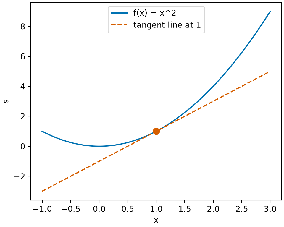
Example 13 (Tangent lines under a parabola)

Example 13 (Tangent lines under a parabola) For $f(x) = x^2$, the right side of Equation 1 is $y^2 + 2y (x - y) = 2xy - y^2$, and

\[ \begin{aligned} f(x) - (2xy - y^2) &= x^2 - 2xy + y^2 \\ &= (x - y)^2 \\ &\ge 0, \end{aligned} \]

with equality only at $x = y$, confirming that $x^2$ is strictly convex. For $g(x) = -x^2$ the inequality fails: at $y = 0$ the tangent line is $s = 0$, and $g(1) = -1 < 0$.

Show code

tl_x_ft <- seq(-1, 3, length.out = 201)
tl_curve_ft <- tibble::tibble(x = tl_x_ft, s = tl_x_ft^2)
tl_line_ft <- tibble::tibble(x = tl_x_ft, s = 2 * tl_x_ft - 1)
tl_point_ft <- tibble::tibble(x = 1, s = 1)
tl_aes_ft <- ggplot2::aes(x, s)
ggplot2::ggplot(tl_curve_ft, tl_aes_ft) +
  ggplot2::geom_line(colour = "#0072B2") +
  ggplot2::geom_line(
    data = tl_line_ft, colour = "#D55E00", linetype = "dashed"
  ) +
  ggplot2::geom_point(data = tl_point_ft, colour = "#D55E00", size = 3) +
  ggplot2::labs(x = "x", y = "s")

Show code

import matplotlib.pyplot as plt
import numpy as np

tl_x_ft = np.linspace(-1, 3, 201)
fig, ax = plt.subplots(figsize=(5, 4), layout="constrained")
ax.plot(tl_x_ft, tl_x_ft**2, color="#0072B2", label="f(x) = x^2")
ax.plot(tl_x_ft, 2 * tl_x_ft - 1, "--", color="#D55E00",
        label="tangent line at 1")
ax.plot(1, 1, "o", color="#D55E00", markersize=8)
ax.set_xlabel("x")
ax.set_ylabel("s")
ax.legend(loc="upper center")
plt.show()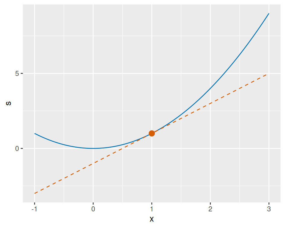

Plot of the parabola f of x equals x squared for x from -1 to 3, in blue, and the straight line s equals 2 x minus 1 in dashed vermilion. The line touches the parabola at the point (1, 1), marked by a vermilion circle, and lies below the parabola everywhere else. — Figure 9: The tangent line $s = 2x - 1$ of $f(x) = x^2$ at $y = 1$ (Example 12). It touches the graph at $(1, 1)$ and lies below it everywhere else, as in Example 13.

Theorem 6 (Second-derivative test for convexity)

Theorem 6 (Second-derivative test for convexity) Let $f : \mathbb{R}^p \to \mathbb{R}$ have first and second partial derivatives that are continuous on $\mathbb{R}^p$.

If $\mathbf{H}_f(\mathord{\smash[b]{\underset{\raise.3ex\hbox{$\scriptstyle\sim$}}{x}}\vphantom{x}})$ is positive semidefinite for every $\mathord{\smash[b]{\underset{\raise.3ex\hbox{$\scriptstyle\sim$}}{x}}\vphantom{x}}$, then $f$ is convex.
If $\mathbf{H}_f(\mathord{\smash[b]{\underset{\raise.3ex\hbox{$\scriptstyle\sim$}}{x}}\vphantom{x}})$ is positive definite for every $\mathord{\smash[b]{\underset{\raise.3ex\hbox{$\scriptstyle\sim$}}{x}}\vphantom{x}}$, then $f$ is strictly convex (Definition 4).

Proof

Proof. Let $\mathord{\smash[b]{\underset{\raise.3ex\hbox{$\scriptstyle\sim$}}{x}}\vphantom{x}}, \mathord{\smash[b]{\underset{\raise.3ex\hbox{$\scriptstyle\sim$}}{y}}\vphantom{y}}\in \mathbb{R}^p$. By Theorem 6 in Critical Points and Optimality Conditions with $\mathord{\smash[b]{\underset{\raise.3ex\hbox{$\scriptstyle\sim$}}{z}}\vphantom{z}} = \mathord{\smash[b]{\underset{\raise.3ex\hbox{$\scriptstyle\sim$}}{y}}\vphantom{y}}$ and $\mathord{\smash[b]{\underset{\raise.3ex\hbox{$\scriptstyle\sim$}}{h}}\vphantom{h}} = \mathord{\smash[b]{\underset{\raise.3ex\hbox{$\scriptstyle\sim$}}{x}}\vphantom{x}}- \mathord{\smash[b]{\underset{\raise.3ex\hbox{$\scriptstyle\sim$}}{y}}\vphantom{y}}$, there is a $\tau\in (0, 1)$ such that, with $\mathord{\smash[b]{\underset{\raise.3ex\hbox{$\scriptstyle\sim$}}{w}}\vphantom{w}} \stackrel{\text{def}}{=}\mathord{\smash[b]{\underset{\raise.3ex\hbox{$\scriptstyle\sim$}}{y}}\vphantom{y}}+ \tau(\mathord{\smash[b]{\underset{\raise.3ex\hbox{$\scriptstyle\sim$}}{x}}\vphantom{x}}- \mathord{\smash[b]{\underset{\raise.3ex\hbox{$\scriptstyle\sim$}}{y}}\vphantom{y}})$,

\[ \begin{aligned} f(\mathord{\smash[b]{\underset{\raise.3ex\hbox{$\scriptstyle\sim$}}{x}}\vphantom{x}}) &= f(\mathord{\smash[b]{\underset{\raise.3ex\hbox{$\scriptstyle\sim$}}{y}}\vphantom{y}}) + {\mathopen{}\left(\frac{\partial}{\partial \mathord{\smash[b]{\underset{\raise.3ex\hbox{$\scriptstyle\sim$}}{x}}\vphantom{x}}} f(\mathord{\smash[b]{\underset{\raise.3ex\hbox{$\scriptstyle\sim$}}{y}}\vphantom{y}})\right)\mathclose{}}^{\top} (\mathord{\smash[b]{\underset{\raise.3ex\hbox{$\scriptstyle\sim$}}{x}}\vphantom{x}}- \mathord{\smash[b]{\underset{\raise.3ex\hbox{$\scriptstyle\sim$}}{y}}\vphantom{y}}) + \frac{1}{2}\,{(\mathord{\smash[b]{\underset{\raise.3ex\hbox{$\scriptstyle\sim$}}{x}}\vphantom{x}}- \mathord{\smash[b]{\underset{\raise.3ex\hbox{$\scriptstyle\sim$}}{y}}\vphantom{y}})}^{\top}\,\mathbf{H}_f(\mathord{\smash[b]{\underset{\raise.3ex\hbox{$\scriptstyle\sim$}}{w}}\vphantom{w}})\,(\mathord{\smash[b]{\underset{\raise.3ex\hbox{$\scriptstyle\sim$}}{x}}\vphantom{x}}- \mathord{\smash[b]{\underset{\raise.3ex\hbox{$\scriptstyle\sim$}}{y}}\vphantom{y}}) && \text{(}\href{optimization-critical-points.qmd#thm-taylor-mv}{\text{Theorem~6 in Critical Points and Optimality Conditions}}\text{)} \\ &\ge f(\mathord{\smash[b]{\underset{\raise.3ex\hbox{$\scriptstyle\sim$}}{y}}\vphantom{y}}) + {\mathopen{}\left(\frac{\partial}{\partial \mathord{\smash[b]{\underset{\raise.3ex\hbox{$\scriptstyle\sim$}}{x}}\vphantom{x}}} f(\mathord{\smash[b]{\underset{\raise.3ex\hbox{$\scriptstyle\sim$}}{y}}\vphantom{y}})\right)\mathclose{}}^{\top} (\mathord{\smash[b]{\underset{\raise.3ex\hbox{$\scriptstyle\sim$}}{x}}\vphantom{x}}- \mathord{\smash[b]{\underset{\raise.3ex\hbox{$\scriptstyle\sim$}}{y}}\vphantom{y}}). && \text{(} \mathbf{H}_f(\mathord{\smash[b]{\underset{\raise.3ex\hbox{$\scriptstyle\sim$}}{w}}\vphantom{w}}) \text{ is positive semidefinite)} \end{aligned} \]

This inequality is Equation 1, so $f$ is convex by Theorem 5. Under the hypothesis of part 2 and with $\mathord{\smash[b]{\underset{\raise.3ex\hbox{$\scriptstyle\sim$}}{x}}\vphantom{x}}\ne \mathord{\smash[b]{\underset{\raise.3ex\hbox{$\scriptstyle\sim$}}{y}}\vphantom{y}}$, the quadratic-form term is positive, so the inequality is strict, and $f$ is strictly convex by the last sentence of Theorem 5.

Example 14 (Using the Hessian to show convexity)

Example 14 (Using the Hessian to show convexity)

For a symmetric positive semidefinite $\mathbf{A}$, $f(\mathord{\smash[b]{\underset{\raise.3ex\hbox{$\scriptstyle\sim$}}{x}}\vphantom{x}}) = {\mathord{\smash[b]{\underset{\raise.3ex\hbox{$\scriptstyle\sim$}}{x}}\vphantom{x}}}^{\top} \mathbf{A} \mathord{\smash[b]{\underset{\raise.3ex\hbox{$\scriptstyle\sim$}}{x}}\vphantom{x}}$ has Hessian $2 \mathbf{A}$ (by the Hessian of a quadratic form), which is positive semidefinite because ${\mathord{\smash[b]{\underset{\raise.3ex\hbox{$\scriptstyle\sim$}}{h}}\vphantom{h}}}^{\top} (2 \mathbf{A}) \mathord{\smash[b]{\underset{\raise.3ex\hbox{$\scriptstyle\sim$}}{h}}\vphantom{h}} = 2\,{\mathord{\smash[b]{\underset{\raise.3ex\hbox{$\scriptstyle\sim$}}{h}}\vphantom{h}}}^{\top} \mathbf{A} \mathord{\smash[b]{\underset{\raise.3ex\hbox{$\scriptstyle\sim$}}{h}}\vphantom{h}} \ge 0$; so $f$ is convex.
$f(\mathord{\smash[b]{\underset{\raise.3ex\hbox{$\scriptstyle\sim$}}{x}}\vphantom{x}}) = x_1^2 + x_2^2 - 2 x_1$ has Hessian $2 \mathbf{I}_2$ (Example 16 in Critical Points and Optimality Conditions), which is positive definite, so $f$ is strictly convex.
$f(\mathord{\smash[b]{\underset{\raise.3ex\hbox{$\scriptstyle\sim$}}{x}}\vphantom{x}}) = e^{2x_1 + x_2} - x_1$ has Hessian $e^{u} \begin{bmatrix} 4 & 2 \\ 2 & 1 \end{bmatrix}$ with $u = 2x_1 + x_2$ (the Hessian example), and

\[ \begin{aligned} {\mathord{\smash[b]{\underset{\raise.3ex\hbox{$\scriptstyle\sim$}}{h}}\vphantom{h}}}^{\top}\,\mathbf{H}_f(\mathord{\smash[b]{\underset{\raise.3ex\hbox{$\scriptstyle\sim$}}{x}}\vphantom{x}})\,\mathord{\smash[b]{\underset{\raise.3ex\hbox{$\scriptstyle\sim$}}{h}}\vphantom{h}} &= e^{u} (4 h_1^2 + 4 h_1 h_2 + h_2^2) \\ &= e^{u} (2 h_1 + h_2)^2 \\ &\ge 0, \end{aligned} \]

so $f$ is convex. The Hessian is not positive definite ($\mathord{\smash[b]{\underset{\raise.3ex\hbox{$\scriptstyle\sim$}}{h}}\vphantom{h}} = {(1, -2)}^{\top}$ gives $0$), so part 2 does not apply, and in fact $f$ is not strictly convex: along $\mathord{\smash[b]{\underset{\raise.3ex\hbox{$\scriptstyle\sim$}}{x}}\vphantom{x}}= t\,{(1, -2)}^{\top}$,

\[ \begin{aligned} u &= 2t - 2t \\ &= 0 \end{aligned} \]

and $f = 1 - t$ is linear in $t$, so the convexity inequality holds with equality there.

Show code

ch_x1_ch <- seq(-1, 1, length.out = 101)
ch_x2_ch <- seq(-3, 3, length.out = 101)
ch_grid_ch <- tidyr::expand_grid(x1 = ch_x1_ch, x2 = ch_x2_ch)
ch_u_ch <- 2 * ch_grid_ch$x1 + ch_grid_ch$x2
ch_grid_ch$z <- exp(ch_u_ch) - ch_grid_ch$x1
ch_line_x1_ch <- c(-1, 1)
ch_line_x2_ch <- c(2, -2)
ch_line_ch <- tibble::tibble(x1 = ch_line_x1_ch, x2 = ch_line_x2_ch)
ch_aes_ch <- ggplot2::aes(x1, x2)
ch_z_aes_ch <- ggplot2::aes(z = z)
ggplot2::ggplot(ch_grid_ch, ch_aes_ch) +
  ggplot2::geom_contour(ch_z_aes_ch, colour = "#0072B2", bins = 12) +
  ggplot2::geom_line(
    data = ch_line_ch, colour = "#D55E00", linetype = "dashed"
  ) +
  ggplot2::labs(x = "x1", y = "x2")

Show code

import matplotlib.pyplot as plt
import numpy as np

ch_x1_ax = np.linspace(-1, 1, 101)
ch_x2_ax = np.linspace(-3, 3, 101)
ch_xx_ax, ch_yy_ax = np.meshgrid(ch_x1_ax, ch_x2_ax)
ch_z_ax = np.exp(2 * ch_xx_ax + ch_yy_ax) - ch_xx_ax
fig, ax = plt.subplots(figsize=(5, 4), layout="constrained")
ax.contour(ch_xx_ax, ch_yy_ax, ch_z_ax, levels=12, colors="#0072B2")
ax.plot([-1, 1], [2, -2], "--", color="#D55E00")
ax.set_xlabel("x1")
ax.set_ylabel("x2")
plt.show();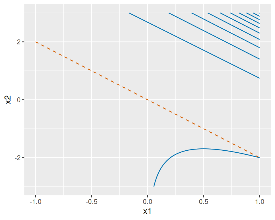

Contour plot of f(x) = exp(2 x1 + x2) - x1 for x1 from -1 to 1 and x2 from -3 to 3. The level curves are long parallel curves that run along the direction (1, -2), crowded together on the upper right and spread out on the lower left. A dashed vermilion line along that direction through the origin marks where f is linear. — Figure 10: Level curves of the third function in Example 14. Along the dashed line through the origin in the direction ${(1, -2)}^{\top}$ the function is linear, so the function is convex but not strictly convex.

Show code

ch_x1_sf <- seq(-1, 1, length.out = 101)
ch_x2_sf <- seq(-3, 3, length.out = 101)
ch_grid_sf <- tidyr::expand_grid(x1 = ch_x1_sf, x2 = ch_x2_sf)
ch_u_sf <- 2 * ch_grid_sf$x1 + ch_grid_sf$x2
ch_value_sf <- exp(ch_u_sf) - ch_grid_sf$x1
ch_n2_sf <- length(ch_x2_sf)
ch_z_sf <- matrix(ch_value_sf, nrow = ch_n2_sf)
ch_l_x1_sf <- seq(-1, 1, length.out = 21)
ch_line_sf <- tibble::tibble(x1 = ch_l_x1_sf)
ch_line_sf$x2 <- -2 * ch_line_sf$x1
ch_lu_sf <- 2 * ch_line_sf$x1 + ch_line_sf$x2
ch_line_sf$z <- exp(ch_lu_sf) - ch_line_sf$x1
ch_dash_sf <- list(color = "#D55E00", dash = "dash", width = 5)
ch_stops_sf <- c(0, 1)
ch_cols_sf <- c("#CCE0F0", "#0072B2")
ch_scale_sf <- list(ch_stops_sf, ch_cols_sf)
ch_eye_sf <- list(x = 1.6, y = -1.6, z = 0.9)
ch_camera_sf <- list(eye = ch_eye_sf)
ch_xaxis_sf <- list(title = "x1")
ch_yaxis_sf <- list(title = "x2")
ch_zaxis_sf <- list(title = "f(x)")
ch_scene_sf <- list(
  xaxis = ch_xaxis_sf,
  yaxis = ch_yaxis_sf,
  zaxis = ch_zaxis_sf,
  camera = ch_camera_sf
)
ch_legend_sf <- list(orientation = "h")
plotly::plot_ly() |>
  plotly::add_surface(
    x = ch_x1_sf,
    y = ch_x2_sf,
    z = ch_z_sf,
    colorscale = ch_scale_sf,
    showscale = FALSE,
    opacity = 0.8
  ) |>
  plotly::add_trace(
    data = ch_line_sf,
    x = ~x1,
    y = ~x2,
    z = ~z,
    type = "scatter3d",
    mode = "lines",
    line = ch_dash_sf,
    name = "f is linear"
  ) |>
  plotly::layout(scene = ch_scene_sf, legend = ch_legend_sf)

Show code

import html
import numpy as np
import plotly.graph_objects as go

fig_alt = (
    "Surface plot of f(x) = exp(2 x1 + x2) - x1 for x1 from -1 to 1 and x2 from "
    "-3 to 3. The surface is a trough that rises steeply toward the upper "
    "right, where 2 x1 plus x2 is large, and is nearly flat on the lower left. "
    "A dashed vermilion straight line along the direction (1, -2) through the "
    "origin lies on the surface, because f is linear there."
)

ch_x1_3d = np.linspace(-1, 1, 101)
ch_x2_3d = np.linspace(-3, 3, 101)
ch_xx_3d, ch_yy_3d = np.meshgrid(ch_x1_3d, ch_x2_3d)
ch_z_3d = np.exp(2 * ch_xx_3d + ch_yy_3d) - ch_xx_3d
ch_line_x1_3d = np.linspace(-1, 1, 21)
ch_line_x2_3d = -2 * ch_line_x1_3d
ch_line_z_3d = np.exp(2 * ch_line_x1_3d + ch_line_x2_3d) - ch_line_x1_3d
fig = go.Figure(data=[
    go.Surface(
        x=ch_x1_3d,
        y=ch_x2_3d,
        z=ch_z_3d,
        colorscale=[[0, "#CCE0F0"], [1, "#0072B2"]],
        showscale=False,
        opacity=0.6,
        showlegend=False,
    ),
    go.Scatter3d(x=ch_line_x1_3d, y=ch_line_x2_3d, z=ch_line_z_3d,
                 mode="lines",
                 line=dict(color="#D55E00", width=5, dash="dash"),
                 name="f is linear"),
])
fig.update_layout(
    scene=dict(
        xaxis_title="x1",
        yaxis_title="x2",
        zaxis_title="f(x)",
        camera=dict(eye=dict(x=1.6, y=-1.6, z=0.9)),
    ),
    legend=dict(orientation="h"),
);
print(
    "```{=html}\n"
    + f'<div role="img" aria-label="{html.escape(fig_alt)}">\n'
    + fig.to_html(full_html=False, include_plotlyjs="cdn")
    + "\n</div>\n```"
)

Figure 11: The graph of the third function in Example 14, the surface whose level curves are in Figure 10. Along the dashed line through the origin in the direction ${(1, -2)}^{\top}$ the surface is a straight line, so the function is linear there. The function is therefore convex but not strictly convex.

R
Python

Example 15 (Strictly convex with a singular Hessian)

Example 15 (Strictly convex with a singular Hessian) Part 2 is sufficient but not necessary. $f(x) = x^4$ has

\[ \begin{aligned} f''(0) &= 12 \cdot 0^2 \\ &= 0, \end{aligned} \]

so $\mathbf{H}_f(0) = [0]$ is singular and not positive definite. Yet $f$ is strictly convex, by the strict form of Equation 1: for $x \ne y$,

\[ \begin{aligned} x^4 - y^4 - 4 y^3 (x - y) &= (x - y)(x^3 + x^2 y + x y^2 + y^3) - 4 y^3 (x - y) && \text{(factor } x^4 - y^4 \text{)} \\ &= (x - y)(x^3 + x^2 y + x y^2 - 3 y^3) && \text{(collect the } y^3 \text{ terms)} \\ &= (x - y)^2 (x^2 + 2 x y + 3 y^2) && \text{(} (x - y)(x^2 + 2 x y + 3 y^2) = x^3 + x^2 y + x y^2 - 3 y^3 \text{)} \\ &= (x - y)^2 \mathopen{}\left((x + y)^2 + 2 y^2\right)\mathclose{}, && \text{(complete the square)} \end{aligned} \]

which is positive: $(x - y)^2 > 0$, and $(x + y)^2 + 2 y^2 = 0$ would need $y = 0$ and then

\[ \begin{aligned} x &= 0 \\ &= y. \end{aligned} \]

Theorem 7 (A convex function has a positive semidefinite Hessian)

Theorem 7 (A convex function has a positive semidefinite Hessian) Let $f : \mathbb{R}^p \to \mathbb{R}$ have first and second partial derivatives that are continuous on $\mathbb{R}^p$. If $f$ is convex, then the Hessian $\mathbf{H}_f(\mathord{\smash[b]{\underset{\raise.3ex\hbox{$\scriptstyle\sim$}}{x}}\vphantom{x}})$ is positive semidefinite for every $\mathord{\smash[b]{\underset{\raise.3ex\hbox{$\scriptstyle\sim$}}{x}}\vphantom{x}}\in \mathbb{R}^p$.

Proof

Proof. Fix $\mathord{\smash[b]{\underset{\raise.3ex\hbox{$\scriptstyle\sim$}}{x}}\vphantom{x}}, \mathord{\smash[b]{\underset{\raise.3ex\hbox{$\scriptstyle\sim$}}{v}}\vphantom{v}} \in \mathbb{R}^p$. Let $h > 0$. By Theorem 6 in Critical Points and Optimality Conditions applied with $\mathord{\smash[b]{\underset{\raise.3ex\hbox{$\scriptstyle\sim$}}{z}}\vphantom{z}} = \mathord{\smash[b]{\underset{\raise.3ex\hbox{$\scriptstyle\sim$}}{x}}\vphantom{x}}$ and $\mathord{\smash[b]{\underset{\raise.3ex\hbox{$\scriptstyle\sim$}}{h}}\vphantom{h}} = h\mathord{\smash[b]{\underset{\raise.3ex\hbox{$\scriptstyle\sim$}}{v}}\vphantom{v}}$, and again with $\mathord{\smash[b]{\underset{\raise.3ex\hbox{$\scriptstyle\sim$}}{h}}\vphantom{h}} = -h\mathord{\smash[b]{\underset{\raise.3ex\hbox{$\scriptstyle\sim$}}{v}}\vphantom{v}}$, there are $\tau_+, \tau_- \in (0, 1)$ with

\[ \begin{aligned} f(\mathord{\smash[b]{\underset{\raise.3ex\hbox{$\scriptstyle\sim$}}{x}}\vphantom{x}}+ h\mathord{\smash[b]{\underset{\raise.3ex\hbox{$\scriptstyle\sim$}}{v}}\vphantom{v}}) &= f(\mathord{\smash[b]{\underset{\raise.3ex\hbox{$\scriptstyle\sim$}}{x}}\vphantom{x}}) + h\,{\mathopen{}\left(\frac{\partial}{\partial \mathord{\smash[b]{\underset{\raise.3ex\hbox{$\scriptstyle\sim$}}{x}}\vphantom{x}}} f(\mathord{\smash[b]{\underset{\raise.3ex\hbox{$\scriptstyle\sim$}}{x}}\vphantom{x}})\right)\mathclose{}}^{\top} \mathord{\smash[b]{\underset{\raise.3ex\hbox{$\scriptstyle\sim$}}{v}}\vphantom{v}} + \frac{h^2}{2}\,{\mathord{\smash[b]{\underset{\raise.3ex\hbox{$\scriptstyle\sim$}}{v}}\vphantom{v}}}^{\top}\,\mathbf{H}_f(\mathord{\smash[b]{\underset{\raise.3ex\hbox{$\scriptstyle\sim$}}{w}}\vphantom{w}}_+)\,\mathord{\smash[b]{\underset{\raise.3ex\hbox{$\scriptstyle\sim$}}{v}}\vphantom{v}} && \text{(}\href{optimization-critical-points.qmd#thm-taylor-mv}{\text{Theorem~6 in Critical Points and Optimality Conditions}}\text{)} \\ f(\mathord{\smash[b]{\underset{\raise.3ex\hbox{$\scriptstyle\sim$}}{x}}\vphantom{x}}- h\mathord{\smash[b]{\underset{\raise.3ex\hbox{$\scriptstyle\sim$}}{v}}\vphantom{v}}) &= f(\mathord{\smash[b]{\underset{\raise.3ex\hbox{$\scriptstyle\sim$}}{x}}\vphantom{x}}) - h\,{\mathopen{}\left(\frac{\partial}{\partial \mathord{\smash[b]{\underset{\raise.3ex\hbox{$\scriptstyle\sim$}}{x}}\vphantom{x}}} f(\mathord{\smash[b]{\underset{\raise.3ex\hbox{$\scriptstyle\sim$}}{x}}\vphantom{x}})\right)\mathclose{}}^{\top} \mathord{\smash[b]{\underset{\raise.3ex\hbox{$\scriptstyle\sim$}}{v}}\vphantom{v}} + \frac{h^2}{2}\,{\mathord{\smash[b]{\underset{\raise.3ex\hbox{$\scriptstyle\sim$}}{v}}\vphantom{v}}}^{\top}\,\mathbf{H}_f(\mathord{\smash[b]{\underset{\raise.3ex\hbox{$\scriptstyle\sim$}}{w}}\vphantom{w}}_-)\,\mathord{\smash[b]{\underset{\raise.3ex\hbox{$\scriptstyle\sim$}}{v}}\vphantom{v}}, && \text{(}\href{optimization-critical-points.qmd#thm-taylor-mv}{\text{Theorem~6 in Critical Points and Optimality Conditions}}\text{)} \end{aligned} \]

where $\mathord{\smash[b]{\underset{\raise.3ex\hbox{$\scriptstyle\sim$}}{w}}\vphantom{w}}_\pm = \mathord{\smash[b]{\underset{\raise.3ex\hbox{$\scriptstyle\sim$}}{x}}\vphantom{x}}\pm \tau_\pm h\mathord{\smash[b]{\underset{\raise.3ex\hbox{$\scriptstyle\sim$}}{v}}\vphantom{v}}$. Adding the two equations cancels the first-order summands:

\[ f(\mathord{\smash[b]{\underset{\raise.3ex\hbox{$\scriptstyle\sim$}}{x}}\vphantom{x}}+ h\mathord{\smash[b]{\underset{\raise.3ex\hbox{$\scriptstyle\sim$}}{v}}\vphantom{v}}) + f(\mathord{\smash[b]{\underset{\raise.3ex\hbox{$\scriptstyle\sim$}}{x}}\vphantom{x}}- h\mathord{\smash[b]{\underset{\raise.3ex\hbox{$\scriptstyle\sim$}}{v}}\vphantom{v}}) - 2 f(\mathord{\smash[b]{\underset{\raise.3ex\hbox{$\scriptstyle\sim$}}{x}}\vphantom{x}}) = \frac{h^2}{2}\,{\mathord{\smash[b]{\underset{\raise.3ex\hbox{$\scriptstyle\sim$}}{v}}\vphantom{v}}}^{\top}\mathopen{}\left(\mathbf{H}_f(\mathord{\smash[b]{\underset{\raise.3ex\hbox{$\scriptstyle\sim$}}{w}}\vphantom{w}}_+) + \mathbf{H}_f(\mathord{\smash[b]{\underset{\raise.3ex\hbox{$\scriptstyle\sim$}}{w}}\vphantom{w}}_-)\right)\mathclose{}\mathord{\smash[b]{\underset{\raise.3ex\hbox{$\scriptstyle\sim$}}{v}}\vphantom{v}}. \]

Since $f$ is convex and $\mathord{\smash[b]{\underset{\raise.3ex\hbox{$\scriptstyle\sim$}}{x}}\vphantom{x}}= \frac{1}{2}(\mathord{\smash[b]{\underset{\raise.3ex\hbox{$\scriptstyle\sim$}}{x}}\vphantom{x}}+ h\mathord{\smash[b]{\underset{\raise.3ex\hbox{$\scriptstyle\sim$}}{v}}\vphantom{v}}) + \frac{1}{2}(\mathord{\smash[b]{\underset{\raise.3ex\hbox{$\scriptstyle\sim$}}{x}}\vphantom{x}}- h\mathord{\smash[b]{\underset{\raise.3ex\hbox{$\scriptstyle\sim$}}{v}}\vphantom{v}})$,

\[ f(\mathord{\smash[b]{\underset{\raise.3ex\hbox{$\scriptstyle\sim$}}{x}}\vphantom{x}}) \le \frac{1}{2} f(\mathord{\smash[b]{\underset{\raise.3ex\hbox{$\scriptstyle\sim$}}{x}}\vphantom{x}}+ h\mathord{\smash[b]{\underset{\raise.3ex\hbox{$\scriptstyle\sim$}}{v}}\vphantom{v}}) + \frac{1}{2} f(\mathord{\smash[b]{\underset{\raise.3ex\hbox{$\scriptstyle\sim$}}{x}}\vphantom{x}}- h\mathord{\smash[b]{\underset{\raise.3ex\hbox{$\scriptstyle\sim$}}{v}}\vphantom{v}}), \]

so the left side of the previous display is nonnegative. Dividing by $h^2 / 2$ gives

\[ {\mathord{\smash[b]{\underset{\raise.3ex\hbox{$\scriptstyle\sim$}}{v}}\vphantom{v}}}^{\top}\mathopen{}\left(\mathbf{H}_f(\mathord{\smash[b]{\underset{\raise.3ex\hbox{$\scriptstyle\sim$}}{w}}\vphantom{w}}_+) + \mathbf{H}_f(\mathord{\smash[b]{\underset{\raise.3ex\hbox{$\scriptstyle\sim$}}{w}}\vphantom{w}}_-)\right)\mathclose{}\mathord{\smash[b]{\underset{\raise.3ex\hbox{$\scriptstyle\sim$}}{v}}\vphantom{v}} \ge 0 \qquad \text{for every } h > 0. \]

As $h \to 0$, both $\mathord{\smash[b]{\underset{\raise.3ex\hbox{$\scriptstyle\sim$}}{w}}\vphantom{w}}_+$ and $\mathord{\smash[b]{\underset{\raise.3ex\hbox{$\scriptstyle\sim$}}{w}}\vphantom{w}}_-$ approach $\mathord{\smash[b]{\underset{\raise.3ex\hbox{$\scriptstyle\sim$}}{x}}\vphantom{x}}$, and the entries of $\mathbf{H}_f$ are continuous, so the left side approaches $2\,{\mathord{\smash[b]{\underset{\raise.3ex\hbox{$\scriptstyle\sim$}}{v}}\vphantom{v}}}^{\top}\,\mathbf{H}_f(\mathord{\smash[b]{\underset{\raise.3ex\hbox{$\scriptstyle\sim$}}{x}}\vphantom{x}})\,\mathord{\smash[b]{\underset{\raise.3ex\hbox{$\scriptstyle\sim$}}{v}}\vphantom{v}}$. Therefore ${\mathord{\smash[b]{\underset{\raise.3ex\hbox{$\scriptstyle\sim$}}{v}}\vphantom{v}}}^{\top}\,\mathbf{H}_f(\mathord{\smash[b]{\underset{\raise.3ex\hbox{$\scriptstyle\sim$}}{x}}\vphantom{x}})\,\mathord{\smash[b]{\underset{\raise.3ex\hbox{$\scriptstyle\sim$}}{v}}\vphantom{v}} \ge 0$ for every $\mathord{\smash[b]{\underset{\raise.3ex\hbox{$\scriptstyle\sim$}}{v}}\vphantom{v}}$.

Corollary 1 (Convex if and only if the Hessian is positive semidefinite)

Corollary 1 (Convex if and only if the Hessian is positive semidefinite) Let $f : \mathbb{R}^p \to \mathbb{R}$ have first and second partial derivatives that are continuous on $\mathbb{R}^p$. Then $f$ is convex if and only if the Hessian $\mathbf{H}_f(\mathord{\smash[b]{\underset{\raise.3ex\hbox{$\scriptstyle\sim$}}{x}}\vphantom{x}})$ is positive semidefinite for every $\mathord{\smash[b]{\underset{\raise.3ex\hbox{$\scriptstyle\sim$}}{x}}\vphantom{x}}\in \mathbb{R}^p$.

Proof

Proof. Part 1 of Theorem 6 proves that a positive semidefinite Hessian at every point makes $f$ convex, and Theorem 7 proves that a convex $f$ has a positive semidefinite Hessian at every point.

Theorem 8 (Second-derivative test for concavity)

Theorem 8 (Second-derivative test for concavity) Let $f : \mathbb{R}^p \to \mathbb{R}$ have first and second partial derivatives that are continuous on $\mathbb{R}^p$.

$f$ is concave if and only if $-\mathbf{H}_f(\mathord{\smash[b]{\underset{\raise.3ex\hbox{$\scriptstyle\sim$}}{x}}\vphantom{x}})$ is positive semidefinite for every $\mathord{\smash[b]{\underset{\raise.3ex\hbox{$\scriptstyle\sim$}}{x}}\vphantom{x}}\in \mathbb{R}^p$.
If $-\mathbf{H}_f(\mathord{\smash[b]{\underset{\raise.3ex\hbox{$\scriptstyle\sim$}}{x}}\vphantom{x}})$ is positive definite for every $\mathord{\smash[b]{\underset{\raise.3ex\hbox{$\scriptstyle\sim$}}{x}}\vphantom{x}}\in \mathbb{R}^p$, then $f$ is strictly concave.

Proof

Proof. Its negative $-f$ has the second partial derivatives $-\frac{\partial}{\partial x_j}\frac{\partial}{\partial x_k} f$, which are continuous on $\mathbb{R}^p$, so its Hessian is $\mathbf{H}_{-f}(\mathord{\smash[b]{\underset{\raise.3ex\hbox{$\scriptstyle\sim$}}{x}}\vphantom{x}}) = -\mathbf{H}_f(\mathord{\smash[b]{\underset{\raise.3ex\hbox{$\scriptstyle\sim$}}{x}}\vphantom{x}})$.

By Definition 5, $f$ is concave if and only if $-f$ is convex. By Corollary 1 applied to $-f$, that holds if and only if $-\mathbf{H}_f(\mathord{\smash[b]{\underset{\raise.3ex\hbox{$\scriptstyle\sim$}}{x}}\vphantom{x}})$ is positive semidefinite for every $\mathord{\smash[b]{\underset{\raise.3ex\hbox{$\scriptstyle\sim$}}{x}}\vphantom{x}}$.
Part 2 of Theorem 6, applied to $-f$, makes $-f$ strictly convex, so $f$ is strictly concave by Definition 6.

Example 16 (A strictly concave quadratic function)

Example 16 (A strictly concave quadratic function) Let $f(\mathord{\smash[b]{\underset{\raise.3ex\hbox{$\scriptstyle\sim$}}{x}}\vphantom{x}}) = 1 - x_1^2 - x_2^2$ for $\mathord{\smash[b]{\underset{\raise.3ex\hbox{$\scriptstyle\sim$}}{x}}\vphantom{x}}= {(x_1, x_2)}^{\top}$. Its Hessian is $\mathbf{H}_f(\mathord{\smash[b]{\underset{\raise.3ex\hbox{$\scriptstyle\sim$}}{x}}\vphantom{x}}) = -2 \mathbf{I}_2$ at every $\mathord{\smash[b]{\underset{\raise.3ex\hbox{$\scriptstyle\sim$}}{x}}\vphantom{x}}$, so $-\mathbf{H}_f(\mathord{\smash[b]{\underset{\raise.3ex\hbox{$\scriptstyle\sim$}}{x}}\vphantom{x}}) = 2 \mathbf{I}_2$. For every $\mathord{\smash[b]{\underset{\raise.3ex\hbox{$\scriptstyle\sim$}}{v}}\vphantom{v}} \ne \mathord{\smash[b]{\underset{\raise.3ex\hbox{$\scriptstyle\sim$}}{0}}\vphantom{0}}$,

\[ \begin{aligned} {\mathord{\smash[b]{\underset{\raise.3ex\hbox{$\scriptstyle\sim$}}{v}}\vphantom{v}}}^{\top} \mathopen{}\left(2 \mathbf{I}_2\right)\mathclose{} \mathord{\smash[b]{\underset{\raise.3ex\hbox{$\scriptstyle\sim$}}{v}}\vphantom{v}} &= 2 {\mathord{\smash[b]{\underset{\raise.3ex\hbox{$\scriptstyle\sim$}}{v}}\vphantom{v}}}^{\top} \mathord{\smash[b]{\underset{\raise.3ex\hbox{$\scriptstyle\sim$}}{v}}\vphantom{v}} && \text{(} \mathbf{I}_2 \mathord{\smash[b]{\underset{\raise.3ex\hbox{$\scriptstyle\sim$}}{v}}\vphantom{v}} = \mathord{\smash[b]{\underset{\raise.3ex\hbox{$\scriptstyle\sim$}}{v}}\vphantom{v}} \text{)} \\ &= 2 \mathopen{}\left\lVert\mathord{\smash[b]{\underset{\raise.3ex\hbox{$\scriptstyle\sim$}}{v}}\vphantom{v}}\right\rVert\mathclose{}^2 && \text{(} {\mathord{\smash[b]{\underset{\raise.3ex\hbox{$\scriptstyle\sim$}}{v}}\vphantom{v}}}^{\top} \mathord{\smash[b]{\underset{\raise.3ex\hbox{$\scriptstyle\sim$}}{v}}\vphantom{v}} = \mathopen{}\left\lVert\mathord{\smash[b]{\underset{\raise.3ex\hbox{$\scriptstyle\sim$}}{v}}\vphantom{v}}\right\rVert\mathclose{}^2 \text{)} \\ &> 0, && \text{(} \mathord{\smash[b]{\underset{\raise.3ex\hbox{$\scriptstyle\sim$}}{v}}\vphantom{v}} \ne \mathord{\smash[b]{\underset{\raise.3ex\hbox{$\scriptstyle\sim$}}{0}}\vphantom{0}}\text{)} \end{aligned} \]

so $-\mathbf{H}_f(\mathord{\smash[b]{\underset{\raise.3ex\hbox{$\scriptstyle\sim$}}{x}}\vphantom{x}})$ is positive definite, and $f$ is strictly concave by part 2 of Theorem 8. Figure 12 shows the dome that its graph forms.

Show code

cc_x_cc <- seq(-1.5, 1.5, length.out = 41)
cc_square_cc <- cc_x_cc^2
cc_sum_cc <- outer(cc_square_cc, cc_square_cc, "+")
cc_dome_cc <- 1 - cc_sum_cc
cc_stops_cc <- c(0, 1)
cc_blue_cols_cc <- c("#CCE0F0", "#0072B2")
cc_blue_cc <- list(cc_stops_cc, cc_blue_cols_cc)
cc_eye_cc <- list(x = 1.6, y = -1.6, z = 0.9)
cc_camera_cc <- list(eye = cc_eye_cc)
cc_xaxis_cc <- list(title = "x1")
cc_yaxis_cc <- list(title = "x2")
cc_zaxis_cc <- list(title = "f(x)")
cc_scene_cc <- list(
  xaxis = cc_xaxis_cc,
  yaxis = cc_yaxis_cc,
  zaxis = cc_zaxis_cc,
  camera = cc_camera_cc
)
plotly::plot_ly() |>
  plotly::add_surface(
    x = cc_x_cc,
    y = cc_x_cc,
    z = cc_dome_cc,
    colorscale = cc_blue_cc,
    showscale = FALSE
  ) |>
  plotly::layout(scene = cc_scene_cc)

Show code

import matplotlib.pyplot as plt
import numpy as np

cc_x1_py, cc_x2_py = np.meshgrid(np.linspace(-1.5, 1.5, 41),
                                 np.linspace(-1.5, 1.5, 41))
cc_dome_py = 1 - cc_x1_py**2 - cc_x2_py**2
fig = plt.figure(figsize=(6, 4.5))
ax = fig.add_subplot(projection="3d")
ax.plot_surface(cc_x1_py, cc_x2_py, cc_dome_py, color="#0072B2", alpha=0.7)
ax.set_xlabel("x1")
ax.set_ylabel("x2")
ax.set_zlabel("f(x)")
plt.show();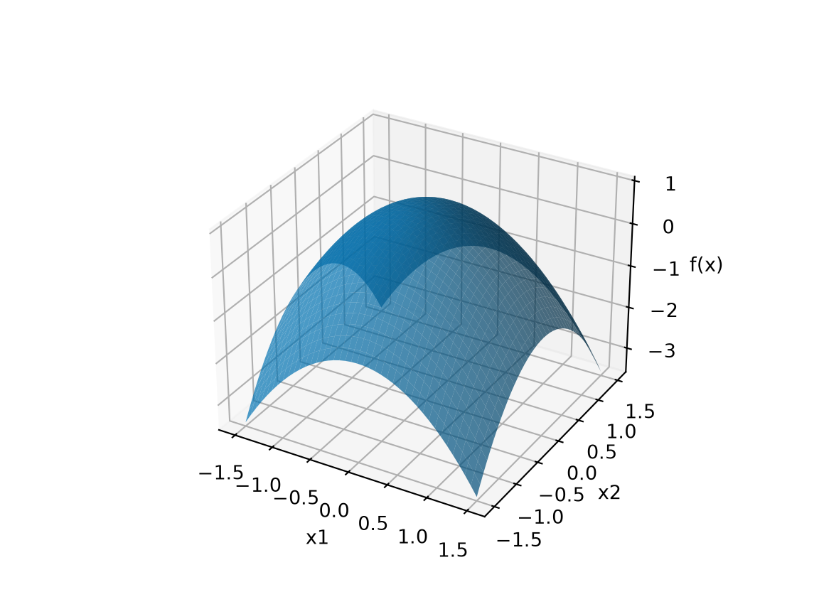

Surface plot of f(x) = 1 - x1^2 - x2^2 for x1 and x2 from -1.5 to 1.5, a dome with its highest point, height 1, at the origin, falling off equally in every direction. — Figure 12: The graph of the strictly concave function $f(\mathord{\smash[b]{\underset{\raise.3ex\hbox{$\scriptstyle\sim$}}{x}}\vphantom{x}}) = 1 - x_1^2 - x_2^2$ of Example 16 is a dome with its highest point at $\mathord{\smash[b]{\underset{\raise.3ex\hbox{$\scriptstyle\sim$}}{0}}\vphantom{0}}$.

Corollary 2 (Stationary points of a convex function are global minimizers)

Corollary 2 (Stationary points of a convex function are global minimizers) If $f$ is as in Theorem 5 and convex, then every stationary point $\mathord{\smash[b]{\underset{\raise.3ex\hbox{$\scriptstyle\sim$}}{x}}\vphantom{x}}^*$ of $f$ (Definition 4 in Critical Points and Optimality Conditions) is a global minimizer.

Proof

Proof. For every $\mathord{\smash[b]{\underset{\raise.3ex\hbox{$\scriptstyle\sim$}}{x}}\vphantom{x}}$,

\[ \begin{aligned} f(\mathord{\smash[b]{\underset{\raise.3ex\hbox{$\scriptstyle\sim$}}{x}}\vphantom{x}}) &\ge f(\mathord{\smash[b]{\underset{\raise.3ex\hbox{$\scriptstyle\sim$}}{x}}\vphantom{x}}^*) + {\mathopen{}\left(\frac{\partial}{\partial \mathord{\smash[b]{\underset{\raise.3ex\hbox{$\scriptstyle\sim$}}{x}}\vphantom{x}}} f(\mathord{\smash[b]{\underset{\raise.3ex\hbox{$\scriptstyle\sim$}}{x}}\vphantom{x}}^*)\right)\mathclose{}}^{\top} (\mathord{\smash[b]{\underset{\raise.3ex\hbox{$\scriptstyle\sim$}}{x}}\vphantom{x}}- \mathord{\smash[b]{\underset{\raise.3ex\hbox{$\scriptstyle\sim$}}{x}}\vphantom{x}}^*) && \text{(}\href{#eq-supporting-hyperplane}{\text{Equation~1}}\text{ with } \mathord{\smash[b]{\underset{\raise.3ex\hbox{$\scriptstyle\sim$}}{y}}\vphantom{y}}= \mathord{\smash[b]{\underset{\raise.3ex\hbox{$\scriptstyle\sim$}}{x}}\vphantom{x}}^* \text{)} \\ &= f(\mathord{\smash[b]{\underset{\raise.3ex\hbox{$\scriptstyle\sim$}}{x}}\vphantom{x}}^*) + {\mathord{\smash[b]{\underset{\raise.3ex\hbox{$\scriptstyle\sim$}}{0}}\vphantom{0}}}^{\top} (\mathord{\smash[b]{\underset{\raise.3ex\hbox{$\scriptstyle\sim$}}{x}}\vphantom{x}}- \mathord{\smash[b]{\underset{\raise.3ex\hbox{$\scriptstyle\sim$}}{x}}\vphantom{x}}^*) && \text{(} \mathord{\smash[b]{\underset{\raise.3ex\hbox{$\scriptstyle\sim$}}{x}}\vphantom{x}}^* \text{ is stationary)} \\ &= f(\mathord{\smash[b]{\underset{\raise.3ex\hbox{$\scriptstyle\sim$}}{x}}\vphantom{x}}^*). && \text{(} \mathord{\smash[b]{\underset{\raise.3ex\hbox{$\scriptstyle\sim$}}{0}}\vphantom{0}} \cdot \mathord{\smash[b]{\underset{\raise.3ex\hbox{$\scriptstyle\sim$}}{v}}\vphantom{v}} = 0 \text{)} \end{aligned} \]

Example 17 (A convex function, and a non-convex one)

Example 17 (A convex function, and a non-convex one)

$f(\mathord{\smash[b]{\underset{\raise.3ex\hbox{$\scriptstyle\sim$}}{x}}\vphantom{x}}) = x_1^2 + x_2^2 - 2 x_1$ is convex by Theorem 6, since its Hessian is $2 \mathbf{I}_2$ (Example 16 in Critical Points and Optimality Conditions), so its stationary point ${(1, 0)}^{\top}$ (Example 8 in Critical Points and Optimality Conditions) is a global minimizer, as completing the square showed in Example 9 in Critical Points and Optimality Conditions.
Without convexity, a stationary point need not be a minimizer at all: $x_1^2 - x_2^2$ has the stationary point $\mathord{\smash[b]{\underset{\raise.3ex\hbox{$\scriptstyle\sim$}}{0}}\vphantom{0}}$, which is not a minimizer (Example 9 in Critical Points and Optimality Conditions).
The corollary says nothing about whether a minimizer exists: $e^{2x_1 + x_2} - x_1$ is convex (Example 14) but has no stationary point, and so no local minimizer (Example 9 in Critical Points and Optimality Conditions).

Definition 11 (Convex optimization problem, convex problem)

Definition 11 (Convex optimization problem, convex problem) A minimization problem whose objective function is convex and whose feasible set is a convex set is a convex optimization problem (or convex problem) [6].

Example 18 (Minimizing over a line, and over a circle)

Example 18 (Minimizing over a line, and over a circle) Let $f(\mathord{\smash[b]{\underset{\raise.3ex\hbox{$\scriptstyle\sim$}}{x}}\vphantom{x}}) = x_1^2 + x_2^2$. Its Hessian is $2 \mathbf{I}_2$ at every $\mathord{\smash[b]{\underset{\raise.3ex\hbox{$\scriptstyle\sim$}}{x}}\vphantom{x}}$, which is positive semidefinite, so $f$ is convex by part 1 of Theorem 6.

Minimizing $f$ subject to $3 x_1 + 4 x_2 = 5$, as in the example of a minimization problem, is a convex problem. Its feasible set $L = \mathopen{}\left\{\mathord{\smash[b]{\underset{\raise.3ex\hbox{$\scriptstyle\sim$}}{x}}\vphantom{x}}\in \mathbb{R}^2 : 3 x_1 + 4 x_2 = 5\right\}\mathclose{}$ is a convex set: for $\mathord{\smash[b]{\underset{\raise.3ex\hbox{$\scriptstyle\sim$}}{x}}\vphantom{x}}, \mathord{\smash[b]{\underset{\raise.3ex\hbox{$\scriptstyle\sim$}}{y}}\vphantom{y}}\in L$ and $t \in [0, 1]$,

\[ \begin{aligned} 3 \mathopen{}\left(t x_1 + (1 - t) y_1\right)\mathclose{} + 4 \mathopen{}\left(t x_2 + (1 - t) y_2\right)\mathclose{} &= t \mathopen{}\left(3 x_1 + 4 x_2\right)\mathclose{} + (1 - t) \mathopen{}\left(3 y_1 + 4 y_2\right)\mathclose{} && \text{(distribute and regroup)} \\ &= 5 t + 5 (1 - t) && \text{(} \mathord{\smash[b]{\underset{\raise.3ex\hbox{$\scriptstyle\sim$}}{x}}\vphantom{x}}, \mathord{\smash[b]{\underset{\raise.3ex\hbox{$\scriptstyle\sim$}}{y}}\vphantom{y}}\in L \text{)} \\ &= 5, && \text{(arithmetic)} \end{aligned} \]

so $t \mathord{\smash[b]{\underset{\raise.3ex\hbox{$\scriptstyle\sim$}}{x}}\vphantom{x}}+ (1 - t) \mathord{\smash[b]{\underset{\raise.3ex\hbox{$\scriptstyle\sim$}}{y}}\vphantom{y}}\in L$.
Minimizing the same $f$ subject to $x_1^2 + x_2^2 = 1$ is not a convex problem, because its feasible set, the unit circle $C$, is not a convex set: ${(1, 0)}^{\top}$ and ${(-1, 0)}^{\top}$ are in $C$, but with $t = \tfrac{1}{2}$ the point $\mathord{\smash[b]{\underset{\raise.3ex\hbox{$\scriptstyle\sim$}}{0}}\vphantom{0}}$ is not, since $0^2 + 0^2 = 0 \ne 1$.

Figure 13 shows both feasible sets.

Show code

cop_x1_fc <- seq(-1.5, 2.5, length.out = 2)
cop_x2_fc <- (5 - 3 * cop_x1_fc) / 4
cop_line_fc <- tibble::tibble(x1 = cop_x1_fc, x2 = cop_x2_fc)
cop_angle_fc <- seq(0, 2 * pi, length.out = 201)
cop_cos_fc <- cos(cop_angle_fc)
cop_sin_fc <- sin(cop_angle_fc)
cop_circle_fc <- tibble::tibble(x1 = cop_cos_fc, x2 = cop_sin_fc)
cop_line_pts_x1_fc <- c(-1, 1)
cop_line_pts_x2_fc <- c(2, 0.5)
cop_line_pts_fc <- tibble::tibble(
  x1 = cop_line_pts_x1_fc,
  x2 = cop_line_pts_x2_fc
)
cop_circle_pts_x1_fc <- c(-1, 1)
cop_circle_pts_x2_fc <- c(0, 0)
cop_circle_pts_fc <- tibble::tibble(
  x1 = cop_circle_pts_x1_fc,
  x2 = cop_circle_pts_x2_fc
)
cop_origin_fc <- tibble::tibble(x1 = 0, x2 = 0)
cop_aes_fc <- ggplot2::aes(x = x1, y = x2)
ggplot2::ggplot() +
  ggplot2::geom_line(
    data = cop_line_fc, mapping = cop_aes_fc, colour = "#0072B2"
  ) +
  ggplot2::geom_point(
    data = cop_line_pts_fc, mapping = cop_aes_fc,
    colour = "#0072B2", size = 3
  ) +
  ggplot2::geom_path(
    data = cop_circle_fc, mapping = cop_aes_fc, colour = "#D55E00"
  ) +
  ggplot2::geom_line(
    data = cop_circle_pts_fc, mapping = cop_aes_fc,
    colour = "#D55E00", linetype = "dashed"
  ) +
  ggplot2::geom_point(
    data = cop_circle_pts_fc, mapping = cop_aes_fc,
    colour = "#D55E00", size = 3
  ) +
  ggplot2::geom_point(
    data = cop_origin_fc, mapping = cop_aes_fc,
    colour = "#D55E00", shape = 21, fill = "white", size = 3
  ) +
  ggplot2::coord_fixed() +
  ggplot2::labs(x = "x1", y = "x2")

Show code

import matplotlib.pyplot as plt
import numpy as np

cop_x1_fc = np.array([-1.5, 2.5])
cop_angle_fc = np.linspace(0, 2 * np.pi, 201)
fig, ax = plt.subplots(figsize=(4.5, 4.5), layout="constrained")
ax.plot(cop_x1_fc, (5 - 3 * cop_x1_fc) / 4, color="#0072B2");
ax.plot([-1, 1], [2, 0.5], "o", color="#0072B2", markersize=8);
ax.plot(np.cos(cop_angle_fc), np.sin(cop_angle_fc), color="#D55E00");
ax.plot([-1, 1], [0, 0], "o--", color="#D55E00", markersize=8);
ax.plot(0, 0, "o", color="#D55E00", markerfacecolor="white", markersize=8);
ax.set_aspect("equal");
ax.set_xlabel("x1");
ax.set_ylabel("x2");
plt.show();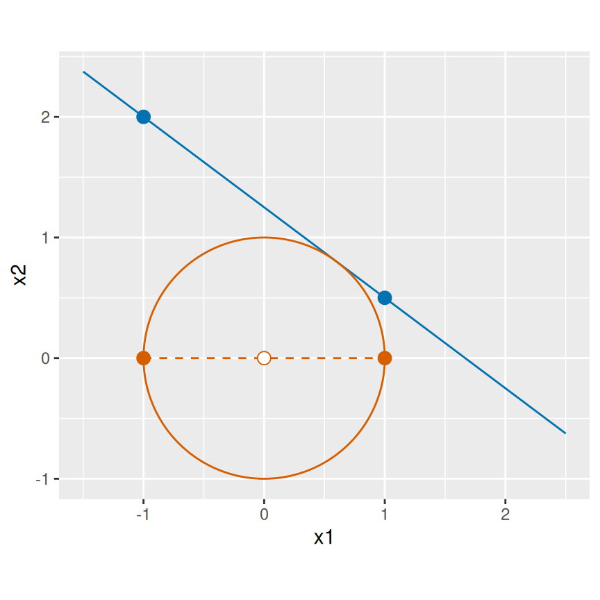

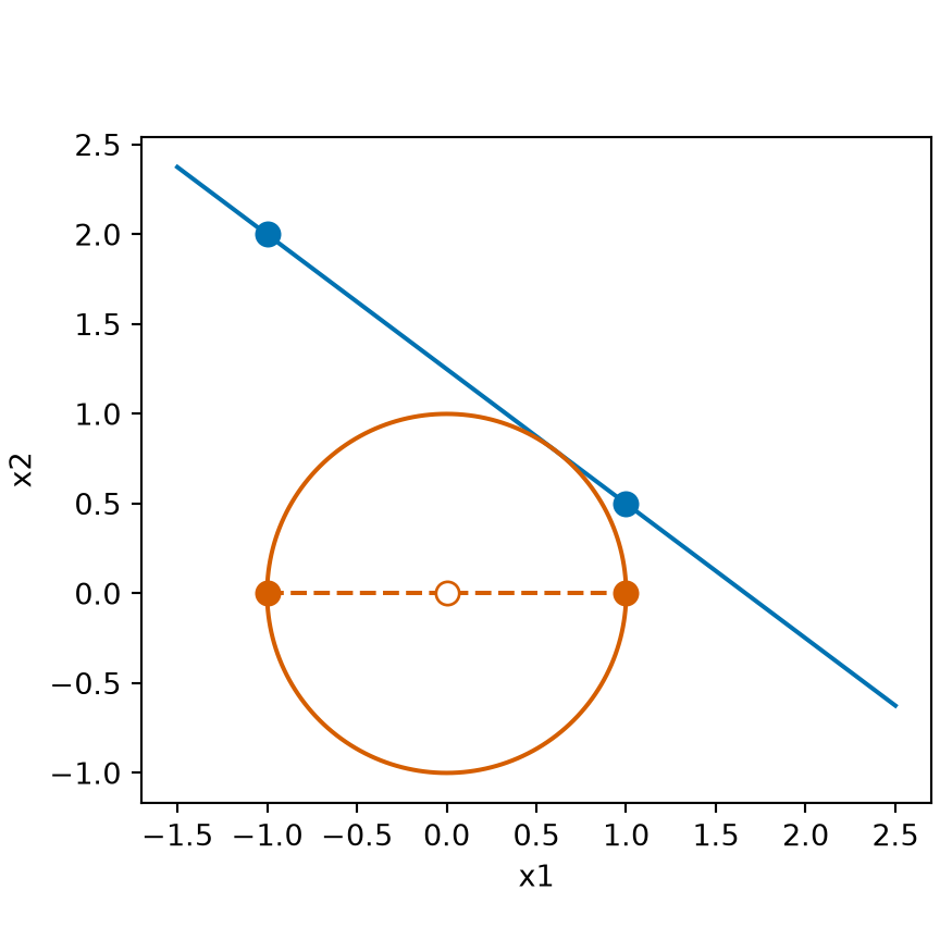
Two feasible sets in the plane. A blue line, 3 x1 + 4 x2 = 5, holds two blue points, (-1, 2) and (1, 0.5), and the segment between them lies on the line. A vermilion unit circle holds two vermilion points, (1, 0) and (-1, 0); the dashed segment between them crosses the inside of the circle, through an open circle at the origin, which is not on the circle. — Figure 13: The two feasible sets of Example 18. The segment between two points of the line stays on the line, so minimizing over the line is a convex problem. The segment between two points of the circle leaves it, through $\mathord{\smash[b]{\underset{\raise.3ex\hbox{$\scriptstyle\sim$}}{0}}\vphantom{0}}$, so minimizing over the circle is not.

Theorem 9 (The exponential function lies above its tangent line at zero)

Theorem 9 (The exponential function lies above its tangent line at zero) For every real $x$,

\[{\operatorname{exp}\mathopen{}\left\{x\right\}\mathclose{}} \ge 1 + x,\]

with equality exactly when $x = 0$.

Proof

Proof. Let $g(x) = {\operatorname{exp}\mathopen{}\left\{x\right\}\mathclose{}} - 1 - x$. The exponential function has second derivative ${\operatorname{exp}\mathopen{}\left\{x\right\}\mathclose{}} > 0$ at every $x$, so it is convex by Theorem 6. The function $g$ differs from it by a linear function, so $g$ is convex too. The derivative of $g$ is $\frac{d g(x)}{d x} = {\operatorname{exp}\mathopen{}\left\{x\right\}\mathclose{}} - 1$, which is $0$ at $x = 0$. By Corollary 2, $0$ is a global minimizer of $g$, and $g(0) = 0$, so $g(x) \ge 0$ for every $x$.

Suppose $g(x) = 0$ for some $x$. Then $x$ is also a global minimizer of $g$, and so a local minimizer. Fermat’s theorem gives $\frac{d g(x)}{d x} = {\operatorname{exp}\mathopen{}\left\{x\right\}\mathclose{}} - 1 = 0$. Then ${\operatorname{exp}\mathopen{}\left\{x\right\}\mathclose{}} = 1 = {\operatorname{exp}\mathopen{}\left\{0\right\}\mathclose{}}$, which gives $x = 0$ because the exponential function is injective.

Corollary 3 (The natural logarithm lies below its tangent line at one)

Corollary 3 (The natural logarithm lies below its tangent line at one) For every $t > 0$,

\[{\operatorname{log}\mathopen{}\left\{t\right\}\mathclose{}} \le t - 1,\]

with equality exactly when $t = 1$.

Proof

Proof. Put $x = {\operatorname{log}\mathopen{}\left\{t\right\}\mathclose{}}$, so that ${\operatorname{exp}\mathopen{}\left\{x\right\}\mathclose{}} = t$ by the inverse relation of the logarithm and the exponential. By Theorem 9, $t = {\operatorname{exp}\mathopen{}\left\{x\right\}\mathclose{}} \ge 1 + x = 1 + {\operatorname{log}\mathopen{}\left\{t\right\}\mathclose{}}$, which is ${\operatorname{log}\mathopen{}\left\{t\right\}\mathclose{}} \le t - 1$. Equality holds exactly when $x = 0$, that is, when ${\operatorname{log}\mathopen{}\left\{t\right\}\mathclose{}} = 0$, that is, when $t = 1$.

Example 19 (Two values of the bounds)

Example 19 (Two values of the bounds)

At $x = 1$, ${\operatorname{exp}\mathopen{}\left\{1\right\}\mathclose{}} = \text{e}\approx 2.718$, which is at least $1 + 1 = 2$. At $t = 2$, ${\operatorname{log}\mathopen{}\left\{2\right\}\mathclose{}} \approx 0.693$, which is at most $2 - 1 = 1$. Neither is an equality, because $x \ne 0$ and $t \ne 1$.

Definitions on this page

Definition 1 (Convex set)
Definition 2 (Half-space)
Definition 3 (Convex hull, convex envelope)
Definition 4 (Strictly convex function)
Definition 5 (Concave function)
Definition 6 (Strictly concave function)
Definition 7 (Convex function on a set)
Definition 8 (Function convex at a point)
Definition 9 (Epigraph)
Definition 10 (Tangent plane)
Definition 11 (Convex optimization problem, convex problem)

References

[1]

H. Zhou, “Optimization and multivariate calculus.” Lecture notes for Biostat 216, Mathematical Methods for Biostatistics, University of California, Los Angeles, 2024. Accessed: Oct. 05, 2026. [Online]. Available: https://ucla-biostat-216.github.io/2024fall/slides/13-optim/13-optim.html

[2]

Wikipedia contributors, “Convex set — Wikipedia, the free encyclopedia.” 2026. Available: https://en.wikipedia.org/wiki/Convex_set

[3]

Wikipedia contributors, “Convex hull — Wikipedia, the free encyclopedia.” 2026. Available: https://en.wikipedia.org/wiki/Convex_hull

[4]

Wikipedia contributors, “Epigraph (mathematics) — Wikipedia, the free encyclopedia.” 2026. Available: https://en.wikipedia.org/wiki/Epigraph_(mathematics)

[5]

Wikipedia contributors, “Tangent space — Wikipedia, the free encyclopedia.” 2026. Available: https://en.wikipedia.org/wiki/Tangent_space

[6]

Wikipedia contributors, “Convex optimization — Wikipedia, the free encyclopedia.” 2026. Available: https://en.wikipedia.org/wiki/Convex_optimization