Convexity in Several Variables

Last modified: 2026-11-13 13:00:00 (PST)

Source

This section is adapted from the convexity part of Zhou [1], used under the MIT License (see the license text in Linear Algebra). The source states the first-order test (in one direction) and the second-derivative test for convexity without proof; here both directions of the first-order test are proved, and the second-derivative test is proved from the Taylor theorem of Section  in Critical Points and Optimality Conditions. The source defines both concave and strictly concave as “\(-f\) is strictly convex”; here \(f\) is concave when \(-f\) is convex. The source states that an intersection of convex sets is convex and that a maximum of convex functions is convex for any finite number of them; here each is stated for two and the general case follows by induction. These parts of the source are not part of this section:

• its catalogs of convex sets and convex functions, including the positive semidefinite matrices and \(-\log \det\)
• intersections of infinitely many convex sets, and suprema of infinitely many convex functions
• its examples, exercises and figures, including the multivariate normal maximum likelihood example

Definition 1 (Convex set) A set \(K \subseteq \mathbb{R}^p\) is convex if [2] for all \(\mathord{\smash[b]{\underset{\raise.3ex\hbox{$\scriptstyle\sim$}}{x}}\vphantom{x}}, \mathord{\smash[b]{\underset{\raise.3ex\hbox{$\scriptstyle\sim$}}{y}}\vphantom{y}}\in K\) and all \(t \in [0, 1]\), the point \(t \mathord{\smash[b]{\underset{\raise.3ex\hbox{$\scriptstyle\sim$}}{x}}\vphantom{x}}+ (1 - t) \mathord{\smash[b]{\underset{\raise.3ex\hbox{$\scriptstyle\sim$}}{y}}\vphantom{y}}\) is in \(K\): \(K\) contains the whole line segment between any two of its points.

Example 1 (Convex sets)  

• \(\mathbb{R}^p\) is convex, and so is any set with at most one point.

• The closed ball \(B = \mathopen{}\left\{\mathord{\smash[b]{\underset{\raise.3ex\hbox{$\scriptstyle\sim$}}{x}}\vphantom{x}}: \mathopen{}\left\lVert\mathord{\smash[b]{\underset{\raise.3ex\hbox{$\scriptstyle\sim$}}{x}}\vphantom{x}}\right\rVert\mathclose{} \le r\right\}\mathclose{}\) is convex: for \(\mathord{\smash[b]{\underset{\raise.3ex\hbox{$\scriptstyle\sim$}}{x}}\vphantom{x}}, \mathord{\smash[b]{\underset{\raise.3ex\hbox{$\scriptstyle\sim$}}{y}}\vphantom{y}}\in B\) and \(t \in [0, 1]\),

  \[ \begin{aligned} \mathopen{}\left\lVert t \mathord{\smash[b]{\underset{\raise.3ex\hbox{$\scriptstyle\sim$}}{x}}\vphantom{x}}+ (1 - t) \mathord{\smash[b]{\underset{\raise.3ex\hbox{$\scriptstyle\sim$}}{y}}\vphantom{y}}\right\rVert\mathclose{} &\le \mathopen{}\left\lVert t \mathord{\smash[b]{\underset{\raise.3ex\hbox{$\scriptstyle\sim$}}{x}}\vphantom{x}}\right\rVert\mathclose{} + \mathopen{}\left\lVert(1 - t) \mathord{\smash[b]{\underset{\raise.3ex\hbox{$\scriptstyle\sim$}}{y}}\vphantom{y}}\right\rVert\mathclose{} && \text{(triangle inequality)} \\ &= t\,\mathopen{}\left\lVert\mathord{\smash[b]{\underset{\raise.3ex\hbox{$\scriptstyle\sim$}}{x}}\vphantom{x}}\right\rVert\mathclose{} + (1 - t)\,\mathopen{}\left\lVert\mathord{\smash[b]{\underset{\raise.3ex\hbox{$\scriptstyle\sim$}}{y}}\vphantom{y}}\right\rVert\mathclose{} && \text{(norm of a multiple; } t, 1 - t \ge 0 \text{)} \\ &\le t\,r + (1 - t)\,r && \text{(} \mathord{\smash[b]{\underset{\raise.3ex\hbox{$\scriptstyle\sim$}}{x}}\vphantom{x}}, \mathord{\smash[b]{\underset{\raise.3ex\hbox{$\scriptstyle\sim$}}{y}}\vphantom{y}}\in B \text{)} \\ &= r. && \text{(arithmetic)} \end{aligned} \]

  The first step is the triangle inequality, and the second uses the norm of a multiple.

Example 2 (A set that is not convex) \(K = \mathopen{}\left\{x \in \mathbb{R}: \mathopen{}\left|x\right|\mathclose{} \ge 1\right\}\mathclose{}\) is not convex: \(-1\) and \(1\) are in \(K\), but with \(t = \tfrac{1}{2}\) the point \(\tfrac{1}{2}(-1) + \tfrac{1}{2}(1) = 0\) is not.

cs_angle_fc <- seq(0, 2 * pi, length.out = 201)
cs_cos_fc <- cos(cs_angle_fc)
cs_sin_fc <- sin(cs_angle_fc)
cs_disk_fc <- tibble::tibble(x1 = cs_cos_fc, x2 = cs_sin_fc)
cs_points_x1_fc <- c(-0.7, 0.6)
cs_points_x2_fc <- c(-0.4, 0.5)
cs_points_fc <- tibble::tibble(x1 = cs_points_x1_fc, x2 = cs_points_x2_fc)
cs_segment_fc <- tibble::tibble(
  x1 = -0.7, x2 = -0.4, x1_end = 0.6, x2_end = 0.5
)
cs_aes_fc <- ggplot2::aes(x1, x2)
cs_seg_aes_fc <- ggplot2::aes(xend = x1_end, yend = x2_end)
ggplot2::ggplot(cs_disk_fc, cs_aes_fc) +
  ggplot2::geom_polygon(fill = "#0072B2", alpha = 0.15, colour = "#0072B2") +
  ggplot2::geom_segment(
    data = cs_segment_fc, mapping = cs_seg_aes_fc, colour = "#D55E00"
  ) +
  ggplot2::geom_point(data = cs_points_fc, colour = "#D55E00", size = 3) +
  ggplot2::coord_fixed() +
  ggplot2::labs(x = "x1", y = "x2")

import matplotlib.pyplot as plt
import numpy as np

cs_angle_fc = np.linspace(0, 2 * np.pi, 201)
cs_x1_fc = np.array([-0.7, 0.6])
cs_x2_fc = np.array([-0.4, 0.5])
fig, ax = plt.subplots(figsize=(4, 4), layout="constrained")
ax.fill(np.cos(cs_angle_fc), np.sin(cs_angle_fc), color="#0072B2", alpha=0.15)
ax.plot(np.cos(cs_angle_fc), np.sin(cs_angle_fc), color="#0072B2")
ax.plot(cs_x1_fc, cs_x2_fc, "o-", color="#D55E00", markersize=8)
ax.set_aspect("equal")
ax.set_xlabel("x1")
ax.set_ylabel("x2")
plt.show()

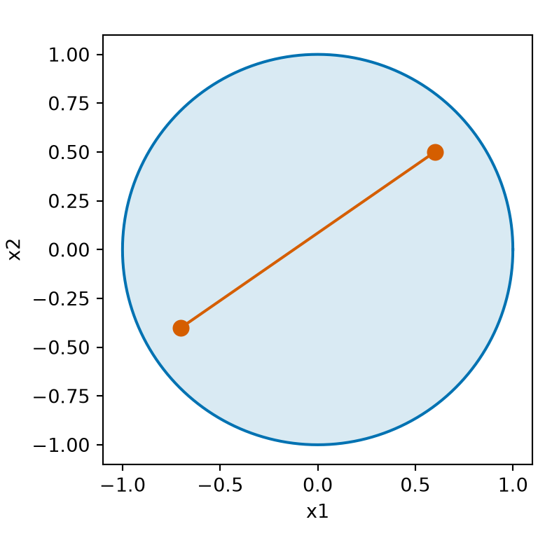
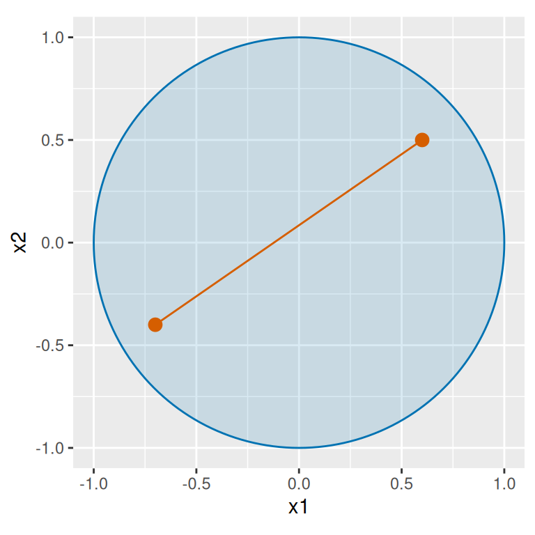
Figure 1: The closed ball of Example 1 in \(\mathbb{R}^2\) with \(r = 1\). The segment between two of its points stays in the ball, as a convex set requires.

• R
• Python

Definition 2 (Half-space) Let \(\mathord{\smash[b]{\underset{\raise.3ex\hbox{$\scriptstyle\sim$}}{a}}\vphantom{a}} \in \mathbb{R}^p\) be a nonzero vector and \(c\) a real number. The set \(\mathopen{}\left\{\mathord{\smash[b]{\underset{\raise.3ex\hbox{$\scriptstyle\sim$}}{x}}\vphantom{x}}\in \mathbb{R}^p : \mathord{\smash[b]{\underset{\raise.3ex\hbox{$\scriptstyle\sim$}}{a}}\vphantom{a}} \cdot \mathord{\smash[b]{\underset{\raise.3ex\hbox{$\scriptstyle\sim$}}{x}}\vphantom{x}} \ge c\right\}\mathclose{}\) is a (closed) half-space: the points on one side of the boundary \(\mathopen{}\left\{\mathord{\smash[b]{\underset{\raise.3ex\hbox{$\scriptstyle\sim$}}{x}}\vphantom{x}}: \mathord{\smash[b]{\underset{\raise.3ex\hbox{$\scriptstyle\sim$}}{a}}\vphantom{a}} \cdot \mathord{\smash[b]{\underset{\raise.3ex\hbox{$\scriptstyle\sim$}}{x}}\vphantom{x}} = c\right\}\mathclose{}\), together with the boundary. In \(\mathbb{R}^2\), a half-space is called a half-plane.

Example 3 (The right half-plane) With \(\mathord{\smash[b]{\underset{\raise.3ex\hbox{$\scriptstyle\sim$}}{a}}\vphantom{a}} = {(1, 0)}^{\top}\) and \(c = 0\), the half-plane \(\mathopen{}\left\{\mathord{\smash[b]{\underset{\raise.3ex\hbox{$\scriptstyle\sim$}}{x}}\vphantom{x}}\in \mathbb{R}^2 : x_1 \ge 0\right\}\mathclose{}\) is the set of points on or to the right of the \(x_2\)-axis. \({(1, 5)}^{\top}\) is in it, since \(1 \ge 0\); \({(0, -3)}^{\top}\) is in it, on the boundary; and \({(-1, 0)}^{\top}\) is not, since \(-1 < 0\).

Theorem 1 (An intersection of convex sets is convex) If \(K_1\) and \(K_2\) are convex subsets of \(\mathbb{R}^p\) (Definition 1), then \(K_1 \cap K_2\) is convex.

Proof. Let \(\mathord{\smash[b]{\underset{\raise.3ex\hbox{$\scriptstyle\sim$}}{x}}\vphantom{x}}, \mathord{\smash[b]{\underset{\raise.3ex\hbox{$\scriptstyle\sim$}}{y}}\vphantom{y}}\in K_1 \cap K_2\) and \(t \in [0, 1]\). Then \(\mathord{\smash[b]{\underset{\raise.3ex\hbox{$\scriptstyle\sim$}}{x}}\vphantom{x}}, \mathord{\smash[b]{\underset{\raise.3ex\hbox{$\scriptstyle\sim$}}{y}}\vphantom{y}}\in K_1\), so \(t \mathord{\smash[b]{\underset{\raise.3ex\hbox{$\scriptstyle\sim$}}{x}}\vphantom{x}}+ (1 - t) \mathord{\smash[b]{\underset{\raise.3ex\hbox{$\scriptstyle\sim$}}{y}}\vphantom{y}}\in K_1\), since \(K_1\) is convex; in the same way \(t \mathord{\smash[b]{\underset{\raise.3ex\hbox{$\scriptstyle\sim$}}{x}}\vphantom{x}}+ (1 - t) \mathord{\smash[b]{\underset{\raise.3ex\hbox{$\scriptstyle\sim$}}{y}}\vphantom{y}}\in K_2\). So \(t \mathord{\smash[b]{\underset{\raise.3ex\hbox{$\scriptstyle\sim$}}{x}}\vphantom{x}}+ (1 - t) \mathord{\smash[b]{\underset{\raise.3ex\hbox{$\scriptstyle\sim$}}{y}}\vphantom{y}}\in K_1 \cap K_2\).

Example 4 (Intersecting a ball with a half-plane) The closed unit ball in \(\mathbb{R}^2\) is convex (Example 1), and so is the half-plane (Definition 2) \(\mathopen{}\left\{\mathord{\smash[b]{\underset{\raise.3ex\hbox{$\scriptstyle\sim$}}{x}}\vphantom{x}}: x_1 \ge 0\right\}\mathclose{}\): if \(x_1 \ge 0\) and \(y_1 \ge 0\), then \(t x_1 + (1 - t) y_1 \ge 0\) for \(t \in [0, 1]\). By Theorem 1, the closed half-disk \(\mathopen{}\left\{\mathord{\smash[b]{\underset{\raise.3ex\hbox{$\scriptstyle\sim$}}{x}}\vphantom{x}}: \mathopen{}\left\lVert\mathord{\smash[b]{\underset{\raise.3ex\hbox{$\scriptstyle\sim$}}{x}}\vphantom{x}}\right\rVert\mathclose{} \le 1,\ x_1 \ge 0\right\}\mathclose{}\) is convex. A union need not be convex: \(\mathopen{}\left\{x \in \mathbb{R}: x \le -1\right\}\mathclose{}\) and \(\mathopen{}\left\{x \in \mathbb{R}: x \ge 1\right\}\mathclose{}\) are convex, but their union is the set of Example 2.

Figure 2 shows the half-disk.

ci_angle_ci <- seq(-pi / 2, pi / 2, length.out = 101)
ci_half_x1_ci <- cos(ci_angle_ci)
ci_half_x2_ci <- sin(ci_angle_ci)
ci_half_ci <- tibble::tibble(x1 = ci_half_x1_ci, x2 = ci_half_x2_ci)
ci_full_angle_ci <- seq(0, 2 * pi, length.out = 201)
ci_full_x1_ci <- cos(ci_full_angle_ci)
ci_full_x2_ci <- sin(ci_full_angle_ci)
ci_full_ci <- tibble::tibble(x1 = ci_full_x1_ci, x2 = ci_full_x2_ci)
ci_edge_ci <- tibble::tibble(x1 = 0, x2 = -1, x1_end = 0, x2_end = 1)
ci_aes_ci <- ggplot2::aes(x1, x2)
ci_seg_aes_ci <- ggplot2::aes(xend = x1_end, yend = x2_end)
ci_full_ci |>
  ggplot2::ggplot() +
  ci_aes_ci +
  ggplot2::geom_path(colour = "grey60") +
  ggplot2::geom_polygon(
    data = ci_half_ci, fill = "#0072B2", alpha = 0.25, colour = "#0072B2"
  ) +
  ggplot2::geom_segment(
    data = ci_edge_ci, mapping = ci_seg_aes_ci,
    colour = "#D55E00", linewidth = 1
  ) +
  ggplot2::coord_fixed() +
  ggplot2::labs(x = "x1", y = "x2")

import matplotlib.pyplot as plt
import numpy as np

ci_full_py = np.linspace(0, 2 * np.pi, 201)
ci_half_py = np.linspace(-np.pi / 2, np.pi / 2, 101)
fig, ax = plt.subplots(figsize=(4, 4), layout="constrained")
ax.plot(np.cos(ci_full_py), np.sin(ci_full_py), color="grey")
ax.fill(np.cos(ci_half_py), np.sin(ci_half_py), color="#0072B2", alpha=0.25)
ax.plot(np.cos(ci_half_py), np.sin(ci_half_py), color="#0072B2")
ax.plot([0, 0], [-1, 1], color="#D55E00", linewidth=2)
ax.set_aspect("equal")
ax.set_xlabel("x1")
ax.set_ylabel("x2")
plt.show();

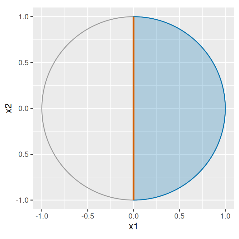
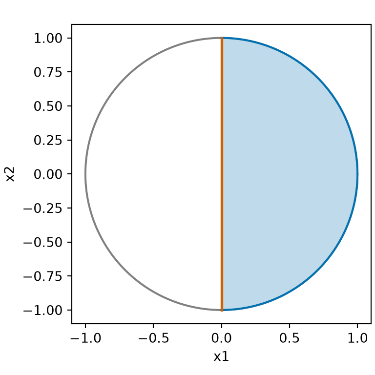
Figure 2: The closed half-disk (blue) is the intersection of the unit ball with the half-plane \(x_1 \ge 0\) of Example 4. The vermilion segment is the edge of the half-plane. The half-disk is convex, as Theorem 1 states.

• R
• Python

Definition 3 (Convex hull, convex envelope) The convex hull (or convex envelope) [3] of a set \(S \subseteq \mathbb{R}^p\) is the set of points that lie in every convex set containing \(S\):

\[ \operatorname{conv}(S) \stackrel{\text{def}}{=}\mathopen{}\left\{\mathord{\smash[b]{\underset{\raise.3ex\hbox{$\scriptstyle\sim$}}{x}}\vphantom{x}}\in \mathbb{R}^p : \mathord{\smash[b]{\underset{\raise.3ex\hbox{$\scriptstyle\sim$}}{x}}\vphantom{x}}\in K \text{ for every convex } K \subseteq \mathbb{R}^p \text{ with } S \subseteq K\right\}\mathclose{}. \]

Example 5 (The convex hull of three points is a triangle) Let \(S = \mathopen{}\left\{\mathord{\smash[b]{\underset{\raise.3ex\hbox{$\scriptstyle\sim$}}{0}}\vphantom{0}}, \mathord{\smash[b]{\underset{\raise.3ex\hbox{$\scriptstyle\sim$}}{e}}\vphantom{e}}_1, \mathord{\smash[b]{\underset{\raise.3ex\hbox{$\scriptstyle\sim$}}{e}}\vphantom{e}}_2\right\}\mathclose{} \subseteq \mathbb{R}^2\), with \(\mathord{\smash[b]{\underset{\raise.3ex\hbox{$\scriptstyle\sim$}}{e}}\vphantom{e}}_1 = {(1, 0)}^{\top}\) and \(\mathord{\smash[b]{\underset{\raise.3ex\hbox{$\scriptstyle\sim$}}{e}}\vphantom{e}}_2 = {(0, 1)}^{\top}\), and let \(T = \mathopen{}\left\{\mathord{\smash[b]{\underset{\raise.3ex\hbox{$\scriptstyle\sim$}}{x}}\vphantom{x}}\in \mathbb{R}^2 : x_1 \ge 0,\ x_2 \ge 0,\ x_1 + x_2 \le 1\right\}\mathclose{}\), the filled triangle with corners \(\mathord{\smash[b]{\underset{\raise.3ex\hbox{$\scriptstyle\sim$}}{0}}\vphantom{0}}\), \(\mathord{\smash[b]{\underset{\raise.3ex\hbox{$\scriptstyle\sim$}}{e}}\vphantom{e}}_1\) and \(\mathord{\smash[b]{\underset{\raise.3ex\hbox{$\scriptstyle\sim$}}{e}}\vphantom{e}}_2\). Then \(\operatorname{conv}(S) = T\): the convex hull of \(S\) is \(T\).

• Inclusion \(\operatorname{conv}(S) \subseteq T\). \(T\) is the intersection of three half-planes, with \(\mathord{\smash[b]{\underset{\raise.3ex\hbox{$\scriptstyle\sim$}}{a}}\vphantom{a}} = {(1, 0)}^{\top}\), \({(0, 1)}^{\top}\) and \({(-1, -1)}^{\top}\), and \(c = 0\), \(0\) and \(-1\). Each half-plane \(H = \mathopen{}\left\{\mathord{\smash[b]{\underset{\raise.3ex\hbox{$\scriptstyle\sim$}}{x}}\vphantom{x}}: \mathord{\smash[b]{\underset{\raise.3ex\hbox{$\scriptstyle\sim$}}{a}}\vphantom{a}} \cdot \mathord{\smash[b]{\underset{\raise.3ex\hbox{$\scriptstyle\sim$}}{x}}\vphantom{x}} \ge c\right\}\mathclose{}\) is convex: for \(\mathord{\smash[b]{\underset{\raise.3ex\hbox{$\scriptstyle\sim$}}{x}}\vphantom{x}}, \mathord{\smash[b]{\underset{\raise.3ex\hbox{$\scriptstyle\sim$}}{y}}\vphantom{y}}\in H\) and \(t \in [0, 1]\),

  \[ \begin{aligned} \mathord{\smash[b]{\underset{\raise.3ex\hbox{$\scriptstyle\sim$}}{a}}\vphantom{a}} \cdot t \mathord{\smash[b]{\underset{\raise.3ex\hbox{$\scriptstyle\sim$}}{x}}\vphantom{x}}+ (1 - t) \mathord{\smash[b]{\underset{\raise.3ex\hbox{$\scriptstyle\sim$}}{y}}\vphantom{y}} &= t \mathord{\smash[b]{\underset{\raise.3ex\hbox{$\scriptstyle\sim$}}{a}}\vphantom{a}} \cdot \mathord{\smash[b]{\underset{\raise.3ex\hbox{$\scriptstyle\sim$}}{x}}\vphantom{x}} + (1 - t) \mathord{\smash[b]{\underset{\raise.3ex\hbox{$\scriptstyle\sim$}}{a}}\vphantom{a}} \cdot \mathord{\smash[b]{\underset{\raise.3ex\hbox{$\scriptstyle\sim$}}{y}}\vphantom{y}} && \text{(the dot product is linear)} \\ &\ge t c + (1 - t) c && \text{(} \mathord{\smash[b]{\underset{\raise.3ex\hbox{$\scriptstyle\sim$}}{x}}\vphantom{x}}, \mathord{\smash[b]{\underset{\raise.3ex\hbox{$\scriptstyle\sim$}}{y}}\vphantom{y}}\in H \text{ and } t, 1 - t \ge 0 \text{)} \\ &= c. && \text{(arithmetic)} \end{aligned} \]

  So \(T\) is convex, by Theorem 1 applied twice. \(T\) contains \(S\), so every point of \(\operatorname{conv}(S)\) is in \(T\).

• Inclusion \(T \subseteq \operatorname{conv}(S)\). Let \(K\) be a convex set containing \(S\), let \(\mathord{\smash[b]{\underset{\raise.3ex\hbox{$\scriptstyle\sim$}}{x}}\vphantom{x}}\in T\), and let \(s = x_1 + x_2\), so \(0 \le s \le 1\). If \(s = 0\), then \(\mathord{\smash[b]{\underset{\raise.3ex\hbox{$\scriptstyle\sim$}}{x}}\vphantom{x}}= \mathord{\smash[b]{\underset{\raise.3ex\hbox{$\scriptstyle\sim$}}{0}}\vphantom{0}}\in K\). Otherwise \(\mathord{\smash[b]{\underset{\raise.3ex\hbox{$\scriptstyle\sim$}}{p}}\vphantom{p}} = \mathord{\smash[b]{\underset{\raise.3ex\hbox{$\scriptstyle\sim$}}{x}}\vphantom{x}}/ s\) has \(p_1 + p_2 = 1\) with \(p_1, p_2 \ge 0\), so \(\mathord{\smash[b]{\underset{\raise.3ex\hbox{$\scriptstyle\sim$}}{p}}\vphantom{p}} = p_1 \mathord{\smash[b]{\underset{\raise.3ex\hbox{$\scriptstyle\sim$}}{e}}\vphantom{e}}_1 + (1 - p_1) \mathord{\smash[b]{\underset{\raise.3ex\hbox{$\scriptstyle\sim$}}{e}}\vphantom{e}}_2\) is in \(K\), by convexity with \(t = p_1\). Then \(\mathord{\smash[b]{\underset{\raise.3ex\hbox{$\scriptstyle\sim$}}{x}}\vphantom{x}}= s \mathord{\smash[b]{\underset{\raise.3ex\hbox{$\scriptstyle\sim$}}{p}}\vphantom{p}} + (1 - s) \mathord{\smash[b]{\underset{\raise.3ex\hbox{$\scriptstyle\sim$}}{0}}\vphantom{0}}\) is in \(K\), by convexity with \(t = s\). So \(\mathord{\smash[b]{\underset{\raise.3ex\hbox{$\scriptstyle\sim$}}{x}}\vphantom{x}}\) is in every convex set containing \(S\).

Figure 3 shows \(S\), \(T\) and the two steps for one point of \(T\).

ch_corner_x1_fc <- c(0, 1, 0)
ch_corner_x2_fc <- c(0, 0, 1)
ch_corners_fc <- tibble::tibble(x1 = ch_corner_x1_fc, x2 = ch_corner_x2_fc)
ch_path_x1_fc <- c(0, 0.2, 0.4)
ch_path_x2_fc <- c(0, 0.3, 0.6)
ch_path_fc <- tibble::tibble(x1 = ch_path_x1_fc, x2 = ch_path_x2_fc)
ch_marks_x1_fc <- c(0.2, 0.4)
ch_marks_x2_fc <- c(0.3, 0.6)
ch_marks_label_fc <- c("x", "p")
ch_marks_fc <- tibble::tibble(
  x1 = ch_marks_x1_fc,
  x2 = ch_marks_x2_fc,
  label = ch_marks_label_fc
)
ch_aes_fc <- ggplot2::aes(x = x1, y = x2)
ch_label_aes_fc <- ggplot2::aes(x = x1, y = x2, label = label)
ggplot2::ggplot() +
  ggplot2::geom_polygon(
    data = ch_corners_fc, mapping = ch_aes_fc,
    fill = "#0072B2", alpha = 0.15, colour = "#0072B2"
  ) +
  ggplot2::geom_point(
    data = ch_corners_fc, mapping = ch_aes_fc,
    colour = "#0072B2", size = 3
  ) +
  ggplot2::geom_line(
    data = ch_path_fc, mapping = ch_aes_fc,
    colour = "#D55E00", linetype = "dashed"
  ) +
  ggplot2::geom_point(
    data = ch_marks_fc, mapping = ch_aes_fc,
    colour = "#D55E00", size = 3
  ) +
  ggplot2::geom_text(
    data = ch_marks_fc, mapping = ch_label_aes_fc,
    colour = "#D55E00", nudge_x = 0.07
  ) +
  ggplot2::coord_fixed() +
  ggplot2::labs(x = "x1", y = "x2")

import matplotlib.pyplot as plt

ch_x1_fc = [0, 1, 0]
ch_x2_fc = [0, 0, 1]
fig, ax = plt.subplots(figsize=(4, 4), layout="constrained")
ax.fill(ch_x1_fc, ch_x2_fc, color="#0072B2", alpha=0.15);
ax.plot(ch_x1_fc + [0], ch_x2_fc + [0], "o-", color="#0072B2", markersize=8);
ax.plot([0, 0.4], [0, 0.6], "--", color="#D55E00");
ax.plot([0.2, 0.4], [0.3, 0.6], "o", color="#D55E00", markersize=8);
ax.annotate("x", (0.2, 0.3), xytext=(6, 0), textcoords="offset points",
            color="#D55E00");
ax.annotate("p", (0.4, 0.6), xytext=(6, 0), textcoords="offset points",
            color="#D55E00");
ax.set_aspect("equal");
ax.set_xlabel("x1");
ax.set_ylabel("x2");
plt.show();

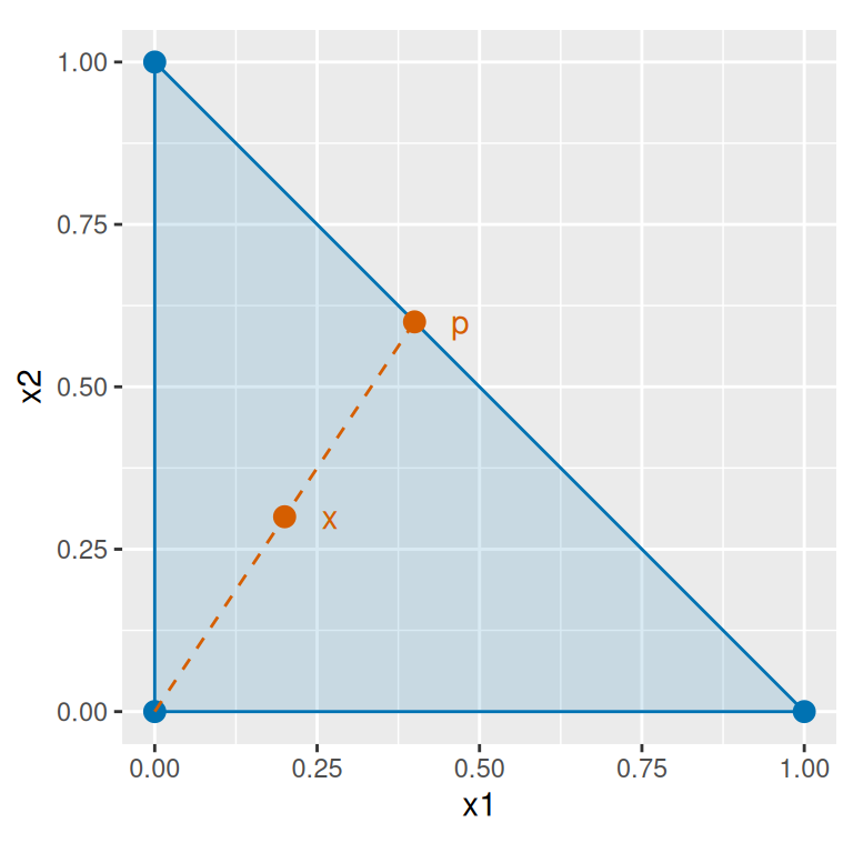
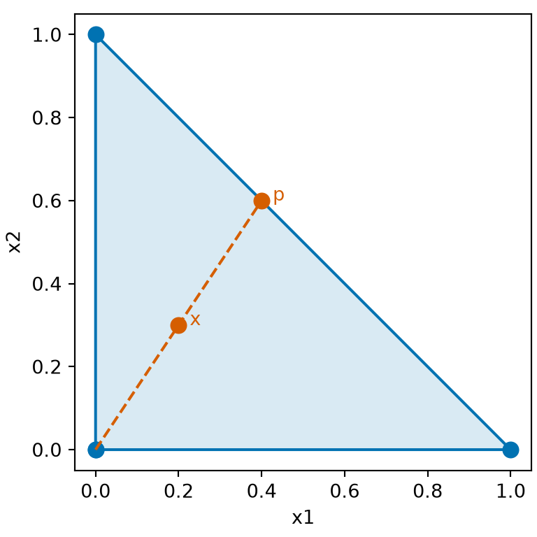
Figure 3: The three blue corners are the set \(S\) of Example 5. The shaded triangle \(T\) is its convex hull. The point \(\mathord{\smash[b]{\underset{\raise.3ex\hbox{$\scriptstyle\sim$}}{x}}\vphantom{x}}= {(0.2, 0.3)}^{\top}\) has \(s = 0.5\). The point \(\mathord{\smash[b]{\underset{\raise.3ex\hbox{$\scriptstyle\sim$}}{p}}\vphantom{p}} = {(0.4, 0.6)}^{\top}\) lies on the segment between \(\mathord{\smash[b]{\underset{\raise.3ex\hbox{$\scriptstyle\sim$}}{e}}\vphantom{e}}_1\) and \(\mathord{\smash[b]{\underset{\raise.3ex\hbox{$\scriptstyle\sim$}}{e}}\vphantom{e}}_2\), and \(\mathord{\smash[b]{\underset{\raise.3ex\hbox{$\scriptstyle\sim$}}{x}}\vphantom{x}}\) lies on the segment between \(\mathord{\smash[b]{\underset{\raise.3ex\hbox{$\scriptstyle\sim$}}{0}}\vphantom{0}}\) and \(\mathord{\smash[b]{\underset{\raise.3ex\hbox{$\scriptstyle\sim$}}{p}}\vphantom{p}}\).

• R
• Python

Definition 4 (Strictly convex function) A function \(f : \mathbb{R}^p \to \mathbb{R}\) is strictly convex if \(f(t \mathord{\smash[b]{\underset{\raise.3ex\hbox{$\scriptstyle\sim$}}{x}}\vphantom{x}}+ (1 - t) \mathord{\smash[b]{\underset{\raise.3ex\hbox{$\scriptstyle\sim$}}{y}}\vphantom{y}}) < t f(\mathord{\smash[b]{\underset{\raise.3ex\hbox{$\scriptstyle\sim$}}{x}}\vphantom{x}}) + (1 - t) f(\mathord{\smash[b]{\underset{\raise.3ex\hbox{$\scriptstyle\sim$}}{y}}\vphantom{y}})\) for all \(\mathord{\smash[b]{\underset{\raise.3ex\hbox{$\scriptstyle\sim$}}{x}}\vphantom{x}}\ne \mathord{\smash[b]{\underset{\raise.3ex\hbox{$\scriptstyle\sim$}}{y}}\vphantom{y}}\) in \(\mathbb{R}^p\) and all \(t \in (0, 1)\).

Definition 5 (Concave function) A function \(f : \mathbb{R}^p \to \mathbb{R}\) is concave if \(-f\) is convex.

Definition 6 (Strictly concave function) A function \(f : \mathbb{R}^p \to \mathbb{R}\) is strictly concave if \(-f\) is strictly convex (Definition 4).

Example 6 (Strictly convex, and convex but not strictly)  

• \(f(x) = x^2\) is strictly convex:

  \[ \begin{aligned} t x^2 + (1 - t) y^2 - (t x + (1 - t) y)^2 &= t x^2 + (1 - t) y^2 - t^2 x^2 - 2 t (1 - t) x y - (1 - t)^2 y^2 && \text{(expand the square)} \\ &= t (1 - t) x^2 - 2 t (1 - t) x y + t (1 - t) y^2 && \text{(} t - t^2 = t (1 - t) \text{, } (1 - t) - (1 - t)^2 = t (1 - t) \text{)} \\ &= t (1 - t) (x - y)^2, && \text{(factor)} \end{aligned} \]

  which is positive when \(x \ne y\) and \(t \in (0, 1)\). At \(t \in \mathopen{}\left\{0, 1\right\}\mathclose{}\) or \(x = y\) it is \(0\), so \(x^2\) is also convex.

• \(f(x) = 2x + 1\) is convex but not strictly convex:

  \[ \begin{aligned} f(t x + (1 - t) y) &= 2 t x + 2 (1 - t) y + 1 \\ &= t f(x) + (1 - t) f(y) \end{aligned} \]

  for every \(x, y, t\), so the inequality holds, but never strictly. It is also concave.

Theorem 2 (An open ball is convex) Let \(\mathord{\smash[b]{\underset{\raise.3ex\hbox{$\scriptstyle\sim$}}{x}}\vphantom{x}}_0 \in \mathbb{R}^p\) and \(r > 0\). The open ball of radius \(r\) around \(\mathord{\smash[b]{\underset{\raise.3ex\hbox{$\scriptstyle\sim$}}{x}}\vphantom{x}}_0\) is a convex set.

Proof. Call the open ball \(B\), and let \(\mathord{\smash[b]{\underset{\raise.3ex\hbox{$\scriptstyle\sim$}}{x}}\vphantom{x}}, \mathord{\smash[b]{\underset{\raise.3ex\hbox{$\scriptstyle\sim$}}{y}}\vphantom{y}}\in B\) and \(t \in [0, 1]\). The triangle inequality and the absolute homogeneity of the norm give

\[ \begin{aligned} \mathopen{}\left\lVert t \mathord{\smash[b]{\underset{\raise.3ex\hbox{$\scriptstyle\sim$}}{x}}\vphantom{x}}+ (1 - t) \mathord{\smash[b]{\underset{\raise.3ex\hbox{$\scriptstyle\sim$}}{y}}\vphantom{y}}- \mathord{\smash[b]{\underset{\raise.3ex\hbox{$\scriptstyle\sim$}}{x}}\vphantom{x}}_0\right\rVert\mathclose{} &= \mathopen{}\left\lVert t (\mathord{\smash[b]{\underset{\raise.3ex\hbox{$\scriptstyle\sim$}}{x}}\vphantom{x}}- \mathord{\smash[b]{\underset{\raise.3ex\hbox{$\scriptstyle\sim$}}{x}}\vphantom{x}}_0) + (1 - t) (\mathord{\smash[b]{\underset{\raise.3ex\hbox{$\scriptstyle\sim$}}{y}}\vphantom{y}}- \mathord{\smash[b]{\underset{\raise.3ex\hbox{$\scriptstyle\sim$}}{x}}\vphantom{x}}_0)\right\rVert\mathclose{} && \text{(} \mathord{\smash[b]{\underset{\raise.3ex\hbox{$\scriptstyle\sim$}}{x}}\vphantom{x}}_0 = t \mathord{\smash[b]{\underset{\raise.3ex\hbox{$\scriptstyle\sim$}}{x}}\vphantom{x}}_0 + (1 - t) \mathord{\smash[b]{\underset{\raise.3ex\hbox{$\scriptstyle\sim$}}{x}}\vphantom{x}}_0 \text{)} \\ &\le t \mathopen{}\left\lVert\mathord{\smash[b]{\underset{\raise.3ex\hbox{$\scriptstyle\sim$}}{x}}\vphantom{x}}- \mathord{\smash[b]{\underset{\raise.3ex\hbox{$\scriptstyle\sim$}}{x}}\vphantom{x}}_0\right\rVert\mathclose{} + (1 - t) \mathopen{}\left\lVert\mathord{\smash[b]{\underset{\raise.3ex\hbox{$\scriptstyle\sim$}}{y}}\vphantom{y}}- \mathord{\smash[b]{\underset{\raise.3ex\hbox{$\scriptstyle\sim$}}{x}}\vphantom{x}}_0\right\rVert\mathclose{} && \text{(triangle inequality and } t, 1 - t \ge 0 \text{)} \\ &< r, && \text{(weighted mean of two numbers less than } r \text{)} \end{aligned} \]

so \(t \mathord{\smash[b]{\underset{\raise.3ex\hbox{$\scriptstyle\sim$}}{x}}\vphantom{x}}+ (1 - t) \mathord{\smash[b]{\underset{\raise.3ex\hbox{$\scriptstyle\sim$}}{y}}\vphantom{y}}\in B\).

Definition 7 (Convex function on a set) Let \(K \subseteq \mathbb{R}^p\) be a convex set. A function \(f : \mathbb{R}^p \to \mathbb{R}\) is convex on \(K\) if

\[ f(t \mathord{\smash[b]{\underset{\raise.3ex\hbox{$\scriptstyle\sim$}}{x}}\vphantom{x}}+ (1 - t) \mathord{\smash[b]{\underset{\raise.3ex\hbox{$\scriptstyle\sim$}}{y}}\vphantom{y}}) \le t f(\mathord{\smash[b]{\underset{\raise.3ex\hbox{$\scriptstyle\sim$}}{x}}\vphantom{x}}) + (1 - t) f(\mathord{\smash[b]{\underset{\raise.3ex\hbox{$\scriptstyle\sim$}}{y}}\vphantom{y}}) \]

for all \(\mathord{\smash[b]{\underset{\raise.3ex\hbox{$\scriptstyle\sim$}}{x}}\vphantom{x}}, \mathord{\smash[b]{\underset{\raise.3ex\hbox{$\scriptstyle\sim$}}{y}}\vphantom{y}}\in K\) and all \(t \in [0, 1]\).

Example 7 (A function convex on an interval but not on the whole line) Let \(f(x) = {\min\mathopen{}\left(x^2, 1\right)\mathclose{}}\).

• \(f\) is convex on \([-1, 1]\), which is the closed ball of radius \(1\) around \(0\) and so convex by Example 1. For \(x, y \in [-1, 1]\) and \(t \in [0, 1]\), the point \(t x + (1 - t) y\) is also in \([-1, 1]\), where \(f\) agrees with \(x^2\), so the defining inequality of \(f\) is the defining inequality of \(x^2\), which holds by Example 6.

• \(f\) is not convex on all of \(\mathbb{R}\): with \(x = 0\), \(y = 2\) and \(t = \tfrac{1}{2}\),

  \[ \begin{aligned} f\mathopen{}\left(\tfrac{1}{2} \cdot 0 + \tfrac{1}{2} \cdot 2\right)\mathclose{} &= f(1) && \text{(} \tfrac{1}{2} \cdot 0 + \tfrac{1}{2} \cdot 2 = 1 \text{)} \\ &= 1, && \text{(} {\min\mathopen{}\left(1, 1\right)\mathclose{}} = 1 \text{)} \end{aligned} \]

  which is greater than \(\tfrac{1}{2} f(0) + \tfrac{1}{2} f(2) = \tfrac{1}{2}\), since \(f(0) = 0\) and \(f(2) = 1\).

In Figure 4, the chord from \(0\) to \(2\) passes below the graph at \(1\), while every chord with both ends in \([-1, 1]\) lies on or above it.

co_x_co <- seq(-2, 2.5, length.out = 451)
co_square_co <- co_x_co^2
co_f_co <- pmin(co_square_co, 1)
co_graph_co <- tibble::tibble(x = co_x_co, f = co_f_co)
co_chord_x_co <- c(0, 2)
co_chord_f_co <- c(0, 1)
co_chord_co <- tibble::tibble(x = co_chord_x_co, f = co_chord_f_co)
co_mid_x_co <- c(1, 1)
co_mid_f_co <- c(0.5, 1)
co_mid_co <- tibble::tibble(x = co_mid_x_co, f = co_mid_f_co)
co_mid_cols_co <- c("#D55E00", "#0072B2")
co_graph_co |>
  ggplot2::ggplot() +
  ggplot2::aes(x = x, y = f) +
  ggplot2::annotate(
    "rect",
    xmin = -1, xmax = 1, ymin = -Inf, ymax = Inf,
    fill = "#0072B2", alpha = 0.1
  ) +
  ggplot2::geom_line(colour = "#0072B2") +
  ggplot2::geom_line(
    data = co_chord_co, colour = "#D55E00", linetype = "dashed"
  ) +
  ggplot2::geom_point(data = co_chord_co, colour = "#D55E00", size = 2) +
  ggplot2::geom_point(data = co_mid_co, colour = co_mid_cols_co, size = 2) +
  ggplot2::labs(x = "x", y = "f(x)") +
  ggplot2::theme_minimal()

import matplotlib.pyplot as plt
import numpy as np

co_x_py = np.linspace(-2, 2.5, 451)
co_f_py = np.minimum(co_x_py**2, 1)
fig, ax = plt.subplots(figsize=(6, 3.5))
ax.axvspan(-1, 1, color="#0072B2", alpha=0.1)
ax.plot(co_x_py, co_f_py, color="#0072B2")
ax.plot([0, 2], [0, 1], "--o", color="#D55E00", markersize=4)
ax.plot([1], [0.5], "o", color="#D55E00", markersize=4)
ax.plot([1], [1], "o", color="#0072B2", markersize=4)
ax.set_xlabel("x")
ax.set_ylabel("f(x)")
plt.show();

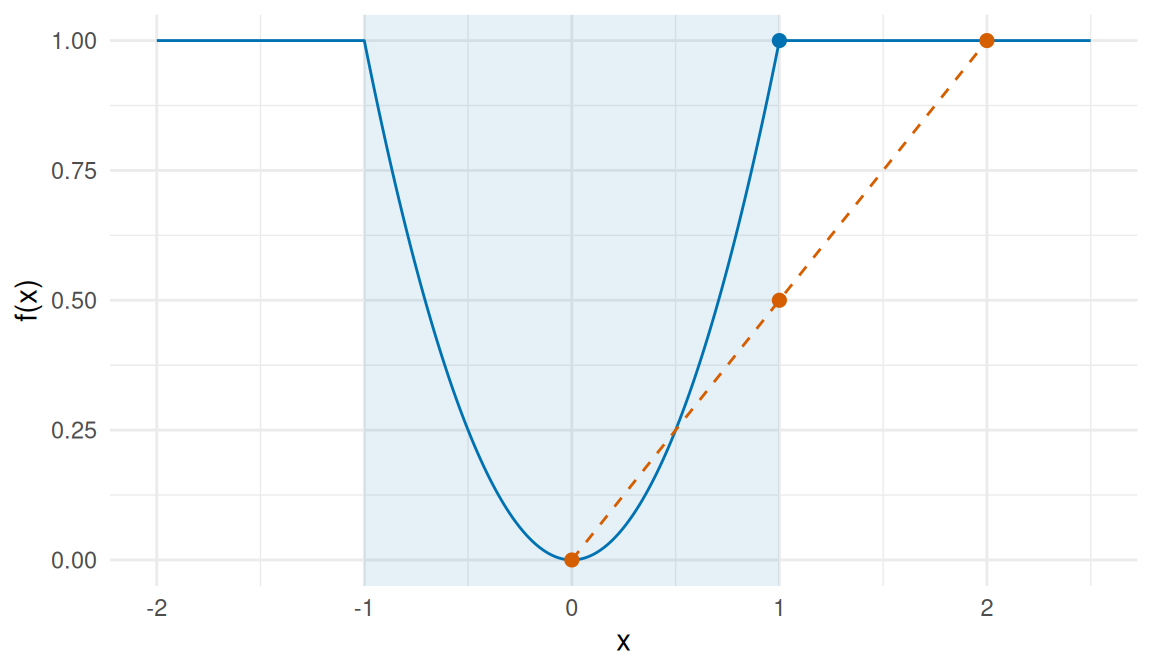
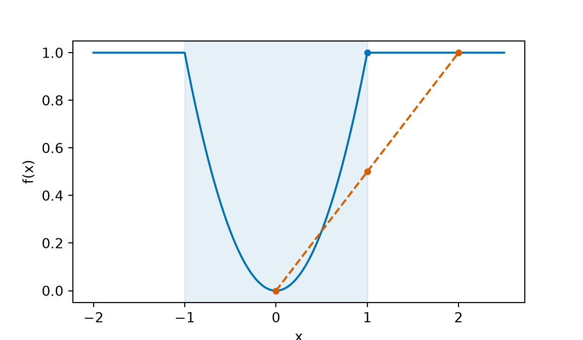
Figure 4: The graph of \(f(x) = {\min\mathopen{}\left(x^2, 1\right)\mathclose{}}\) from Example 7. On the shaded interval \([-1, 1]\), \(f\) is \(x^2\) and is convex on it. The dashed chord from \(0\) to \(2\) is at \(\tfrac{1}{2}\) above \(x = 1\), below \(f(1) = 1\).

• R
• Python

Definition 8 (Function convex at a point) Let \(f : \mathbb{R}^p \to \mathbb{R}\) and let \(\mathord{\smash[b]{\underset{\raise.3ex\hbox{$\scriptstyle\sim$}}{x}}\vphantom{x}}_0 \in \mathbb{R}^p\). \(f\) is convex at \(\mathord{\smash[b]{\underset{\raise.3ex\hbox{$\scriptstyle\sim$}}{x}}\vphantom{x}}_0\) if there is an \(r > 0\) such that \(f\) is convex on the open ball of radius \(r\) around \(\mathord{\smash[b]{\underset{\raise.3ex\hbox{$\scriptstyle\sim$}}{x}}\vphantom{x}}_0\).

Example 8 (A function convex at one point and not at another) Let \(f(x) = {\min\mathopen{}\left(x^2, 1\right)\mathclose{}}\), as in Example 7.

• \(f\) is convex at \(0\): the open ball of radius \(1\) around \(0\) is \((-1, 1)\), a subset of \([-1, 1]\), and \(f\) is convex on \([-1, 1]\) by Example 7, so the defining inequality holds for all \(x, y \in (-1, 1)\) as well.

• \(f\) is not convex at \(1\). Take any \(r > 0\), let \(\varepsilon= \tfrac{1}{2} {\min\mathopen{}\left(r, 1\right)\mathclose{}}\), and take \(x = 1 - \varepsilon\), \(y = 1 + \varepsilon\) and \(t = \tfrac{1}{2}\), so that \(x\) and \(y\) are in the open ball of radius \(r\) around \(1\) and \(t x + (1 - t) y = 1\). Then \(f(1) = 1\), while

  \[ \begin{aligned} \tfrac{1}{2} f(1 - \varepsilon) + \tfrac{1}{2} f(1 + \varepsilon) &= \tfrac{1}{2} (1 - \varepsilon)^2 + \tfrac{1}{2} \cdot 1 && \text{(} 0 < 1 - \varepsilon< 1 < 1 + \varepsilon\text{)} \\ &< \tfrac{1}{2} + \tfrac{1}{2} && \text{(} (1 - \varepsilon)^2 < 1 \text{)} \\ &= 1, && \text{(add)} \end{aligned} \]

  so the defining inequality fails on every open ball around \(1\).

In Figure 5, the chord from \(1 - \varepsilon\) to \(1 + \varepsilon\) passes below the graph at \(1\).

ca_x_ca <- seq(0.4, 1.6, length.out = 241)
ca_square_ca <- ca_x_ca^2
ca_f_ca <- pmin(ca_square_ca, 1)
ca_graph_ca <- tibble::tibble(x = ca_x_ca, f = ca_f_ca)
ca_ends_ca <- c(0.75, 1.25)
ca_end_squares_ca <- ca_ends_ca^2
ca_end_f_ca <- pmin(ca_end_squares_ca, 1)
ca_chord_ca <- tibble::tibble(x = ca_ends_ca, f = ca_end_f_ca)
ca_chord_mid_ca <- mean(ca_end_f_ca)
ca_mid_x_ca <- c(1, 1)
ca_mid_f_ca <- c(ca_chord_mid_ca, 1)
ca_mid_ca <- tibble::tibble(x = ca_mid_x_ca, f = ca_mid_f_ca)
ca_mid_cols_ca <- c("#D55E00", "#0072B2")
ca_graph_ca |>
  ggplot2::ggplot() +
  ggplot2::aes(x = x, y = f) +
  ggplot2::annotate(
    "rect",
    xmin = 0.5, xmax = 1.5, ymin = -Inf, ymax = Inf,
    fill = "#0072B2", alpha = 0.1
  ) +
  ggplot2::geom_line(colour = "#0072B2") +
  ggplot2::geom_line(
    data = ca_chord_ca, colour = "#D55E00", linetype = "dashed"
  ) +
  ggplot2::geom_point(data = ca_chord_ca, colour = "#D55E00", size = 2) +
  ggplot2::geom_point(data = ca_mid_ca, colour = ca_mid_cols_ca, size = 2) +
  ggplot2::labs(x = "x", y = "f(x)") +
  ggplot2::theme_minimal()

import matplotlib.pyplot as plt
import numpy as np

ca_x_py = np.linspace(0.4, 1.6, 241)
ca_f_py = np.minimum(ca_x_py**2, 1)
ca_ends_py = np.array([0.75, 1.25])
ca_end_f_py = np.minimum(ca_ends_py**2, 1)
fig, ax = plt.subplots(figsize=(6, 3.5))
ax.axvspan(0.5, 1.5, color="#0072B2", alpha=0.1)
ax.plot(ca_x_py, ca_f_py, color="#0072B2")
ax.plot(ca_ends_py, ca_end_f_py, "--o", color="#D55E00", markersize=4)
ax.plot([1], [ca_end_f_py.mean()], "o", color="#D55E00", markersize=4)
ax.plot([1], [1], "o", color="#0072B2", markersize=4)
ax.set_xlabel("x")
ax.set_ylabel("f(x)")
plt.show();

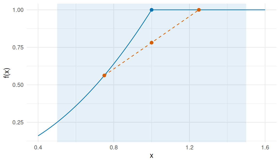
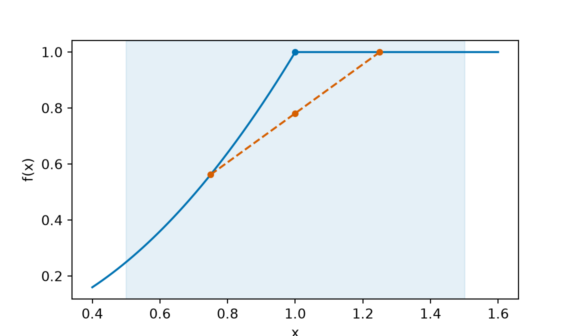
Figure 5: The graph of \(f(x) = {\min\mathopen{}\left(x^2, 1\right)\mathclose{}}\) near \(1\), from Example 8, with \(r = \tfrac{1}{2}\) and \(\varepsilon= \tfrac{1}{4}\). The dashed chord from \(\tfrac{3}{4}\) to \(\tfrac{5}{4}\) stays inside the shaded open ball of radius \(r\) around \(1\), and is at \(\tfrac{25}{32}\) above \(x = 1\), below \(f(1) = 1\).

• R
• Python

Theorem 3 (The maximum of convex functions is convex) If \(f_1\) and \(f_2\) are convex functions on \(\mathbb{R}^p\), then \(f(\mathord{\smash[b]{\underset{\raise.3ex\hbox{$\scriptstyle\sim$}}{x}}\vphantom{x}}) \stackrel{\text{def}}{=}\max\mathopen{}\left\{f_1(\mathord{\smash[b]{\underset{\raise.3ex\hbox{$\scriptstyle\sim$}}{x}}\vphantom{x}}), f_2(\mathord{\smash[b]{\underset{\raise.3ex\hbox{$\scriptstyle\sim$}}{x}}\vphantom{x}})\right\}\mathclose{}\) is convex.

Proof. Let \(\mathord{\smash[b]{\underset{\raise.3ex\hbox{$\scriptstyle\sim$}}{x}}\vphantom{x}}, \mathord{\smash[b]{\underset{\raise.3ex\hbox{$\scriptstyle\sim$}}{y}}\vphantom{y}}\in \mathbb{R}^p\) and \(t \in [0, 1]\). For \(i = 1, 2\),

\[ \begin{aligned} f_i(t \mathord{\smash[b]{\underset{\raise.3ex\hbox{$\scriptstyle\sim$}}{x}}\vphantom{x}}+ (1 - t) \mathord{\smash[b]{\underset{\raise.3ex\hbox{$\scriptstyle\sim$}}{y}}\vphantom{y}}) &\le t f_i(\mathord{\smash[b]{\underset{\raise.3ex\hbox{$\scriptstyle\sim$}}{x}}\vphantom{x}}) + (1 - t) f_i(\mathord{\smash[b]{\underset{\raise.3ex\hbox{$\scriptstyle\sim$}}{y}}\vphantom{y}}) && \text{(} f_i \text{ is convex)} \\ &\le t f(\mathord{\smash[b]{\underset{\raise.3ex\hbox{$\scriptstyle\sim$}}{x}}\vphantom{x}}) + (1 - t) f(\mathord{\smash[b]{\underset{\raise.3ex\hbox{$\scriptstyle\sim$}}{y}}\vphantom{y}}). && \text{(} f_i \le f \text{, and } t, 1 - t \ge 0 \text{)} \end{aligned} \]

Both \(f_1\) and \(f_2\) at \(t \mathord{\smash[b]{\underset{\raise.3ex\hbox{$\scriptstyle\sim$}}{x}}\vphantom{x}}+ (1 - t) \mathord{\smash[b]{\underset{\raise.3ex\hbox{$\scriptstyle\sim$}}{y}}\vphantom{y}}\) are at most \(t f(\mathord{\smash[b]{\underset{\raise.3ex\hbox{$\scriptstyle\sim$}}{x}}\vphantom{x}}) + (1 - t) f(\mathord{\smash[b]{\underset{\raise.3ex\hbox{$\scriptstyle\sim$}}{y}}\vphantom{y}})\), so their maximum \(f(t \mathord{\smash[b]{\underset{\raise.3ex\hbox{$\scriptstyle\sim$}}{x}}\vphantom{x}}+ (1 - t) \mathord{\smash[b]{\underset{\raise.3ex\hbox{$\scriptstyle\sim$}}{y}}\vphantom{y}})\) is too.

Example 9 (A maximum is convex; a minimum need not be)  

• \(f_1(x) = x\) is convex, by the computation for \(2x + 1\) in Example 6 with \(2\) and \(1\) replaced by \(1\) and \(0\), and \(f_2(x) = x^2\) is convex by the same example, so \(\max\mathopen{}\left\{x, x^2\right\}\mathclose{}\) is convex by Theorem 3.

• The minimum of two convex functions need not be convex: \(g(x) = \min\mathopen{}\left\{x^2, (x - 2)^2\right\}\mathclose{}\) has

  \[ \begin{aligned} g(0) &= g(2) \\ &= 0, \end{aligned} \]

  but at the midpoint

  \[ \begin{aligned} g(1) &= \min\mathopen{}\left\{1, 1\right\}\mathclose{} \\ &= 1 \\ &> \tfrac{1}{2} g(0) + \tfrac{1}{2} g(2) \\ &= 0. \end{aligned} \]

cm_x_fm <- seq(-1, 3, length.out = 201)
cm_levels_fm <- c("max{x, x^2}", "min{x^2, (x - 2)^2}")
cm_max_value_fm <- pmax(cm_x_fm, cm_x_fm^2)
cm_min_value_fm <- pmin(cm_x_fm^2, (cm_x_fm - 2)^2)
cm_max_fm <- tibble::tibble(
  x = cm_x_fm, value = cm_max_value_fm, panel = cm_levels_fm[1]
)
cm_min_fm <- tibble::tibble(
  x = cm_x_fm, value = cm_min_value_fm, panel = cm_levels_fm[2]
)
cm_main_fm <- dplyr::bind_rows(cm_max_fm, cm_min_fm)
cm_main_fm$panel <- factor(cm_main_fm$panel, levels = cm_levels_fm)
cm_square_value_fm <- cm_x_fm^2
cm_line_fm <- tibble::tibble(
  x = cm_x_fm, value = cm_x_fm, panel = cm_levels_fm[1], part = "x"
)
cm_square_fm <- tibble::tibble(
  x = cm_x_fm, value = cm_square_value_fm, panel = cm_levels_fm[1],
  part = "x^2"
)
cm_parts_fm <- dplyr::bind_rows(cm_line_fm, cm_square_fm)
cm_parts_fm$panel <- factor(cm_parts_fm$panel, levels = cm_levels_fm)
cm_chord_fm <- tibble::tibble(
  x = 0, xend = 2, value = 0, panel = cm_levels_fm[2]
)
cm_chord_fm$panel <- factor(cm_chord_fm$panel, levels = cm_levels_fm)
cm_mid_fm <- tibble::tibble(x = 1, value = 1, panel = cm_levels_fm[2])
cm_mid_fm$panel <- factor(cm_mid_fm$panel, levels = cm_levels_fm)
cm_aes_fm <- ggplot2::aes(x, value)
cm_parts_aes_fm <- ggplot2::aes(group = part)
cm_chord_aes_fm <- ggplot2::aes(xend = xend, yend = value)
ggplot2::ggplot(cm_main_fm, cm_aes_fm) +
  ggplot2::geom_line(
    data = cm_parts_fm, mapping = cm_parts_aes_fm,
    colour = "grey60", linewidth = 0.4
  ) +
  ggplot2::geom_line(colour = "#0072B2") +
  ggplot2::geom_segment(
    data = cm_chord_fm, mapping = cm_chord_aes_fm, colour = "#D55E00"
  ) +
  ggplot2::geom_point(data = cm_mid_fm, colour = "#D55E00", size = 3) +
  ggplot2::facet_wrap(~panel, scales = "free_y") +
  ggplot2::labs(x = "x", y = NULL)

import matplotlib.pyplot as plt
import numpy as np

cm_x_fm = np.linspace(-1, 3, 201)
fig, axes = plt.subplots(1, 2, figsize=(7, 3.5), layout="constrained")
axes[0].plot(cm_x_fm, cm_x_fm, color="grey", linewidth=0.8)
axes[0].plot(cm_x_fm, cm_x_fm**2, color="grey", linewidth=0.8)
axes[0].plot(cm_x_fm, np.maximum(cm_x_fm, cm_x_fm**2), color="#0072B2")
axes[0].set_title("max{x, x^2}")
axes[1].plot(cm_x_fm, np.minimum(cm_x_fm**2, (cm_x_fm - 2)**2), color="#0072B2")
axes[1].plot([0, 2], [0, 0], "o-", color="#D55E00", markersize=6)
axes[1].plot(1, 1, "o", color="#D55E00", markersize=8)
axes[1].set_title("min{x^2, (x - 2)^2}")
for ax in axes:
    ax.set_xlabel("x")
plt.show()

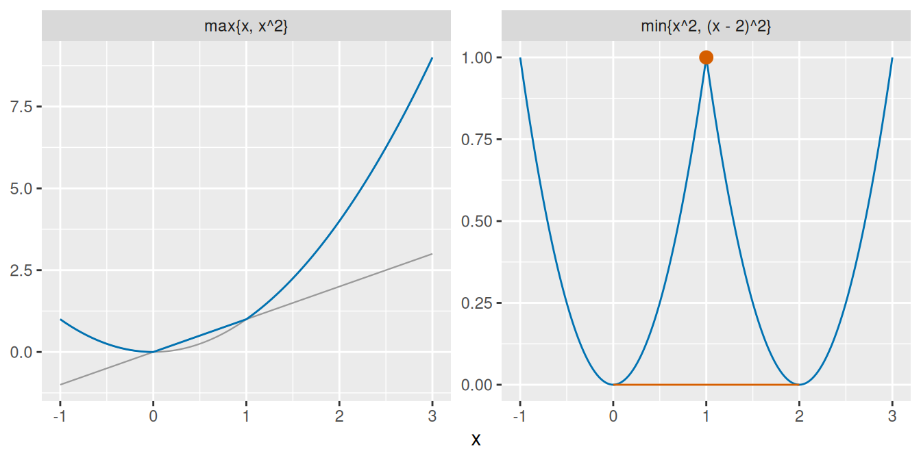
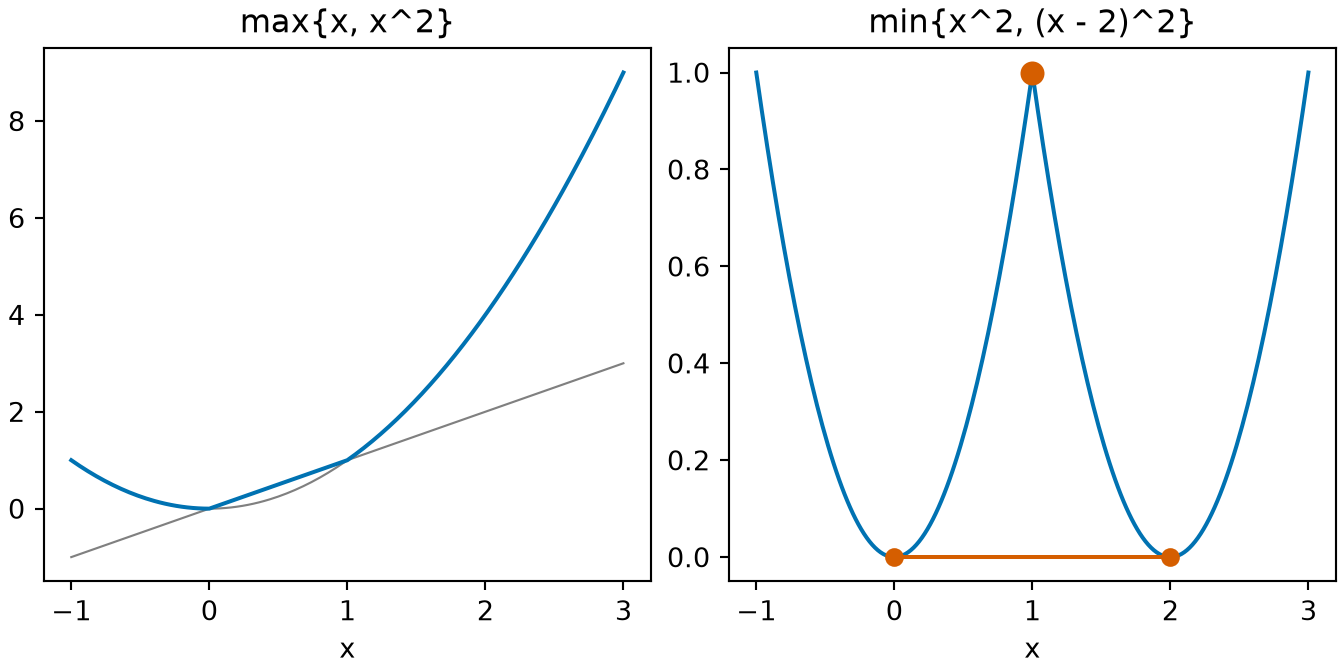
Figure 6: The functions of Example 9. The maximum of the two convex functions on the left is again one. The minimum on the right is not: \(g(1) = 1\) is above \(\tfrac{1}{2} g(0) + \tfrac{1}{2} g(2) = 0\), the height of the segment.

• R
• Python

Definition 9 (Epigraph) The epigraph [4] of \(f : \mathbb{R}^p \to \mathbb{R}\) is the set of points on or over its graph,

\[ \operatorname{epi} f \stackrel{\text{def}}{=}\mathopen{}\left\{(\mathord{\smash[b]{\underset{\raise.3ex\hbox{$\scriptstyle\sim$}}{x}}\vphantom{x}}, s) : \mathord{\smash[b]{\underset{\raise.3ex\hbox{$\scriptstyle\sim$}}{x}}\vphantom{x}}\in \mathbb{R}^p,\ s \in \mathbb{R},\ f(\mathord{\smash[b]{\underset{\raise.3ex\hbox{$\scriptstyle\sim$}}{x}}\vphantom{x}}) \le s\right\}\mathclose{}. \]

A pair \((\mathord{\smash[b]{\underset{\raise.3ex\hbox{$\scriptstyle\sim$}}{x}}\vphantom{x}}, s)\) is treated as the \((p + 1)\)-vector with entries \(x_1, \ldots, x_p, s\), so \(\operatorname{epi} f \subseteq \mathbb{R}^{p+1}\), and sums and multiples of pairs are taken entry by entry.

Example 10 (The epigraph of \(x^2\)) For \(f(x) = x^2\), \(\operatorname{epi} f = \mathopen{}\left\{(x, s) : x^2 \le s\right\}\mathclose{}\), the points \((x, s)\) on the parabola \(s = x^2\) or on the side of it where \(s\) is larger. \((1, 2)\) is in it, since \(1^2 \le 2\); \((2, 1)\) is not, since \(2^2 > 1\).

ep_x_fe <- seq(-2, 2, length.out = 201)
ep_curve_fe <- tibble::tibble(x = ep_x_fe, s = ep_x_fe^2, top = 5)
ep_marks_x_fe <- c(1, 2)
ep_marks_s_fe <- c(2, 1)
ep_marks_kind_fe <- c("in the epigraph", "not in the epigraph")
ep_marks_fe <- tibble::tibble(
  x = ep_marks_x_fe, s = ep_marks_s_fe, kind = ep_marks_kind_fe
)
ep_aes_fe <- ggplot2::aes(x, s)
ep_ribbon_aes_fe <- ggplot2::aes(ymin = s, ymax = top)
ep_marks_aes_fe <- ggplot2::aes(shape = kind)
ep_shapes_fe <- c("in the epigraph" = 16, "not in the epigraph" = 4)
ggplot2::ggplot(ep_curve_fe, ep_aes_fe) +
  ggplot2::geom_ribbon(
    mapping = ep_ribbon_aes_fe, fill = "#0072B2", alpha = 0.15
  ) +
  ggplot2::geom_line(colour = "#0072B2") +
  ggplot2::geom_point(
    data = ep_marks_fe, mapping = ep_marks_aes_fe,
    colour = "#D55E00", size = 3
  ) +
  ggplot2::scale_shape_manual(values = ep_shapes_fe) +
  ggplot2::labs(x = "x", y = "s", shape = NULL)

import matplotlib.pyplot as plt
import numpy as np

ep_x_fe = np.linspace(-2, 2, 201)
fig, ax = plt.subplots(figsize=(5, 4), layout="constrained")
ax.fill_between(ep_x_fe, ep_x_fe**2, 5, color="#0072B2", alpha=0.15)
ax.plot(ep_x_fe, ep_x_fe**2, color="#0072B2")
ax.plot(1, 2, "o", color="#D55E00", markersize=8, label="in the epigraph")
ax.plot(2, 1, "x", color="#D55E00", markersize=8, label="not in the epigraph")
ax.set_ylim(0, 5)
#> (0.0, 5.0)
ax.set_xlabel("x")
ax.set_ylabel("s")
ax.legend(loc="upper center")
plt.show()

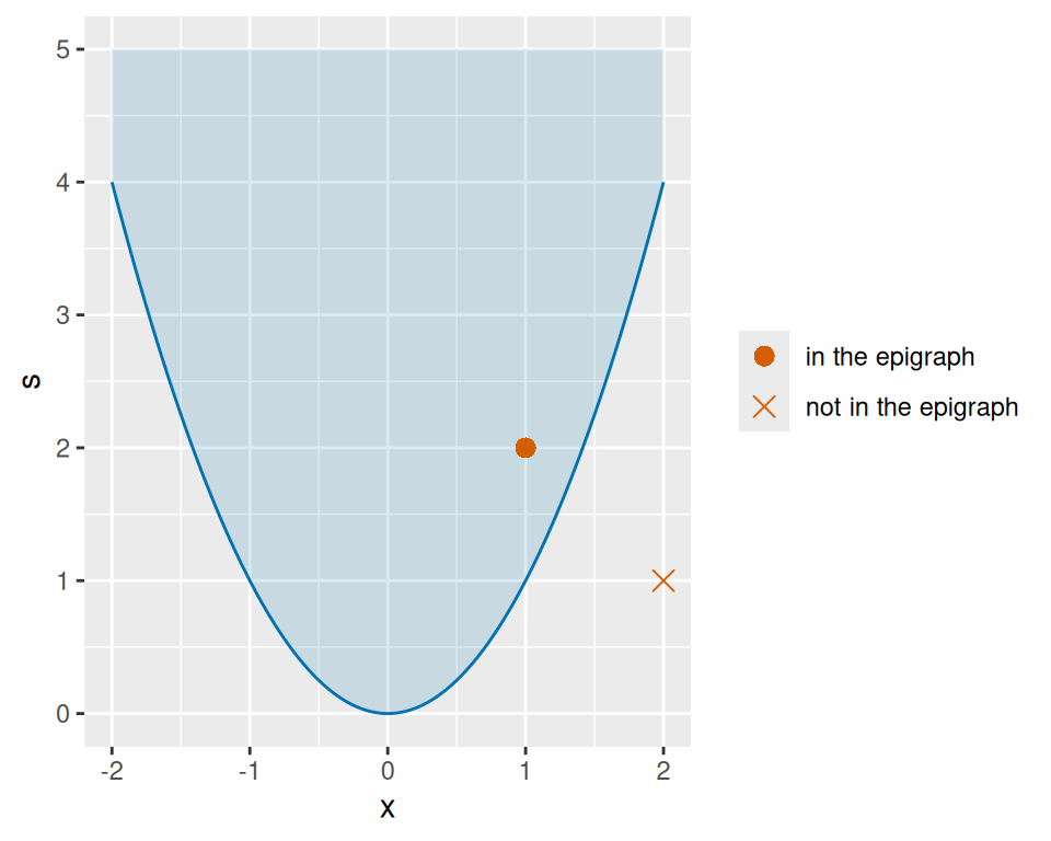
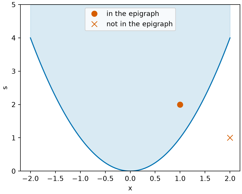
Figure 7: The epigraph of \(f(x) = x^2\) (Example 10): the shaded points on or above the parabola. \((1, 2)\) is in it, and \((2, 1)\) is not.

• R
• Python

Theorem 4 (Convexity through the epigraph) \(f : \mathbb{R}^p \to \mathbb{R}\) is convex if and only if its epigraph (Definition 9) is convex (Definition 1).

Proof. If. Let \(\mathord{\smash[b]{\underset{\raise.3ex\hbox{$\scriptstyle\sim$}}{x}}\vphantom{x}}, \mathord{\smash[b]{\underset{\raise.3ex\hbox{$\scriptstyle\sim$}}{y}}\vphantom{y}}\in \mathbb{R}^p\) and \(t \in [0, 1]\). The points \((\mathord{\smash[b]{\underset{\raise.3ex\hbox{$\scriptstyle\sim$}}{x}}\vphantom{x}}, f(\mathord{\smash[b]{\underset{\raise.3ex\hbox{$\scriptstyle\sim$}}{x}}\vphantom{x}}))\) and \((\mathord{\smash[b]{\underset{\raise.3ex\hbox{$\scriptstyle\sim$}}{y}}\vphantom{y}}, f(\mathord{\smash[b]{\underset{\raise.3ex\hbox{$\scriptstyle\sim$}}{y}}\vphantom{y}}))\) are in \(\operatorname{epi} f\), since \(f(\mathord{\smash[b]{\underset{\raise.3ex\hbox{$\scriptstyle\sim$}}{x}}\vphantom{x}}) \le f(\mathord{\smash[b]{\underset{\raise.3ex\hbox{$\scriptstyle\sim$}}{x}}\vphantom{x}})\) and \(f(\mathord{\smash[b]{\underset{\raise.3ex\hbox{$\scriptstyle\sim$}}{y}}\vphantom{y}}) \le f(\mathord{\smash[b]{\underset{\raise.3ex\hbox{$\scriptstyle\sim$}}{y}}\vphantom{y}})\). Since \(\operatorname{epi} f\) is convex, it contains

\[ t\,(\mathord{\smash[b]{\underset{\raise.3ex\hbox{$\scriptstyle\sim$}}{x}}\vphantom{x}}, f(\mathord{\smash[b]{\underset{\raise.3ex\hbox{$\scriptstyle\sim$}}{x}}\vphantom{x}})) + (1 - t)\,(\mathord{\smash[b]{\underset{\raise.3ex\hbox{$\scriptstyle\sim$}}{y}}\vphantom{y}}, f(\mathord{\smash[b]{\underset{\raise.3ex\hbox{$\scriptstyle\sim$}}{y}}\vphantom{y}})) = \mathopen{}\left(t \mathord{\smash[b]{\underset{\raise.3ex\hbox{$\scriptstyle\sim$}}{x}}\vphantom{x}}+ (1 - t) \mathord{\smash[b]{\underset{\raise.3ex\hbox{$\scriptstyle\sim$}}{y}}\vphantom{y}},\ t f(\mathord{\smash[b]{\underset{\raise.3ex\hbox{$\scriptstyle\sim$}}{x}}\vphantom{x}}) + (1 - t) f(\mathord{\smash[b]{\underset{\raise.3ex\hbox{$\scriptstyle\sim$}}{y}}\vphantom{y}})\right)\mathclose{}, \]

and by Definition 9 that membership means \(f(t \mathord{\smash[b]{\underset{\raise.3ex\hbox{$\scriptstyle\sim$}}{x}}\vphantom{x}}+ (1 - t) \mathord{\smash[b]{\underset{\raise.3ex\hbox{$\scriptstyle\sim$}}{y}}\vphantom{y}}) \le t f(\mathord{\smash[b]{\underset{\raise.3ex\hbox{$\scriptstyle\sim$}}{x}}\vphantom{x}}) + (1 - t) f(\mathord{\smash[b]{\underset{\raise.3ex\hbox{$\scriptstyle\sim$}}{y}}\vphantom{y}})\).

Only if. Let \((\mathord{\smash[b]{\underset{\raise.3ex\hbox{$\scriptstyle\sim$}}{x}}\vphantom{x}}, s)\) and \((\mathord{\smash[b]{\underset{\raise.3ex\hbox{$\scriptstyle\sim$}}{y}}\vphantom{y}}, u)\) be in \(\operatorname{epi} f\), so \(f(\mathord{\smash[b]{\underset{\raise.3ex\hbox{$\scriptstyle\sim$}}{x}}\vphantom{x}}) \le s\) and \(f(\mathord{\smash[b]{\underset{\raise.3ex\hbox{$\scriptstyle\sim$}}{y}}\vphantom{y}}) \le u\), and let \(t \in [0, 1]\). Then

\[ \begin{aligned} f(t \mathord{\smash[b]{\underset{\raise.3ex\hbox{$\scriptstyle\sim$}}{x}}\vphantom{x}}+ (1 - t) \mathord{\smash[b]{\underset{\raise.3ex\hbox{$\scriptstyle\sim$}}{y}}\vphantom{y}}) &\le t f(\mathord{\smash[b]{\underset{\raise.3ex\hbox{$\scriptstyle\sim$}}{x}}\vphantom{x}}) + (1 - t) f(\mathord{\smash[b]{\underset{\raise.3ex\hbox{$\scriptstyle\sim$}}{y}}\vphantom{y}}) && \text{(} f \text{ is convex)} \\ &\le t s + (1 - t) u, && \text{(} f(\mathord{\smash[b]{\underset{\raise.3ex\hbox{$\scriptstyle\sim$}}{x}}\vphantom{x}}) \le s \text{, } f(\mathord{\smash[b]{\underset{\raise.3ex\hbox{$\scriptstyle\sim$}}{y}}\vphantom{y}}) \le u \text{, and } t, 1 - t \ge 0 \text{)} \end{aligned} \]

so \(t\,(\mathord{\smash[b]{\underset{\raise.3ex\hbox{$\scriptstyle\sim$}}{x}}\vphantom{x}}, s) + (1 - t)\,(\mathord{\smash[b]{\underset{\raise.3ex\hbox{$\scriptstyle\sim$}}{y}}\vphantom{y}}, u) = (t \mathord{\smash[b]{\underset{\raise.3ex\hbox{$\scriptstyle\sim$}}{x}}\vphantom{x}}+ (1 - t) \mathord{\smash[b]{\underset{\raise.3ex\hbox{$\scriptstyle\sim$}}{y}}\vphantom{y}},\ t s + (1 - t) u)\) is in \(\operatorname{epi} f\).

Example 11 (Two epigraphs)  

• The epigraph of \(f(x) = \mathopen{}\left|x\right|\mathclose{}\) is \(\mathopen{}\left\{(x, s) : \mathopen{}\left|x\right|\mathclose{} \le s\right\}\mathclose{}\), a wedge. It is the intersection of the half-planes \(\mathopen{}\left\{(x, s) : s - x \ge 0\right\}\mathclose{}\) and \(\mathopen{}\left\{(x, s) : s + x \ge 0\right\}\mathclose{}\). Each half-plane is convex: if \(s_1 - x_1 \ge 0\) and \(s_2 - x_2 \ge 0\), then \((t s_1 + (1 - t) s_2) - (t x_1 + (1 - t) x_2) = t (s_1 - x_1) + (1 - t)(s_2 - x_2) \ge 0\), and the same with \(+\) for the other. So the wedge is convex (Theorem 1), and \(\mathopen{}\left|x\right|\mathclose{}\) is convex by Theorem 4.
• The epigraph of \(g(x) = -x^2\) is not convex: \((-1, -1)\) and \((1, -1)\) are in it, since \(g(\pm 1) = -1\), but their midpoint \((0, -1)\) is not, since \(g(0) = 0 > -1\). So \(-x^2\) is not convex.

Definition 10 (Tangent plane) Let \(f : \mathbb{R}^p \to \mathbb{R}\) have a gradient at \(\mathord{\smash[b]{\underset{\raise.3ex\hbox{$\scriptstyle\sim$}}{y}}\vphantom{y}}\). The tangent plane [5] to the graph of \(f\) at \(\mathord{\smash[b]{\underset{\raise.3ex\hbox{$\scriptstyle\sim$}}{y}}\vphantom{y}}\) is the graph of the function

\[ \mathord{\smash[b]{\underset{\raise.3ex\hbox{$\scriptstyle\sim$}}{x}}\vphantom{x}}\mapsto f(\mathord{\smash[b]{\underset{\raise.3ex\hbox{$\scriptstyle\sim$}}{y}}\vphantom{y}}) + {\mathopen{}\left(\frac{\partial}{\partial \mathord{\smash[b]{\underset{\raise.3ex\hbox{$\scriptstyle\sim$}}{x}}\vphantom{x}}} f(\mathord{\smash[b]{\underset{\raise.3ex\hbox{$\scriptstyle\sim$}}{y}}\vphantom{y}})\right)\mathclose{}}^{\top} (\mathord{\smash[b]{\underset{\raise.3ex\hbox{$\scriptstyle\sim$}}{x}}\vphantom{x}}- \mathord{\smash[b]{\underset{\raise.3ex\hbox{$\scriptstyle\sim$}}{y}}\vphantom{y}}), \]

which takes the value \(f(\mathord{\smash[b]{\underset{\raise.3ex\hbox{$\scriptstyle\sim$}}{y}}\vphantom{y}})\) at \(\mathord{\smash[b]{\underset{\raise.3ex\hbox{$\scriptstyle\sim$}}{x}}\vphantom{x}}= \mathord{\smash[b]{\underset{\raise.3ex\hbox{$\scriptstyle\sim$}}{y}}\vphantom{y}}\) and has the same gradient as \(f\) there.

Example 12 (A tangent line and a tangent plane)  

• For \(f(x) = x^2\) at \(y = 1\), \(f(1) = 1\) and \(f'(1) = 2\), so the tangent line is

  \[ \begin{aligned} s &= 1 + 2\,(x - 1) && \text{(substitute } f(1) \text{ and } f'(1) \text{)} \\ &= 1 + 2x - 2 && \text{(distribute)} \\ &= 2x - 1. && \text{(} 1 - 2 = -1 \text{)} \end{aligned} \]

• For \(f(\mathord{\smash[b]{\underset{\raise.3ex\hbox{$\scriptstyle\sim$}}{x}}\vphantom{x}}) = x_1^2 + x_2^2\) at \(\mathord{\smash[b]{\underset{\raise.3ex\hbox{$\scriptstyle\sim$}}{y}}\vphantom{y}}= {(1, 1)}^{\top}\), \(f(\mathord{\smash[b]{\underset{\raise.3ex\hbox{$\scriptstyle\sim$}}{y}}\vphantom{y}}) = 2\) and the gradient is \(\nabla f(\mathord{\smash[b]{\underset{\raise.3ex\hbox{$\scriptstyle\sim$}}{y}}\vphantom{y}}) = {(2 y_1,\ 2 y_2)}^{\top} = {(2, 2)}^{\top}\), so the tangent plane is

  \[ \begin{aligned} s &= 2 + 2\,(x_1 - 1) + 2\,(x_2 - 1) && \text{(substitute } f(\mathord{\smash[b]{\underset{\raise.3ex\hbox{$\scriptstyle\sim$}}{y}}\vphantom{y}}) \text{ and the gradient)} \\ &= 2 + 2 x_1 - 2 + 2 x_2 - 2 && \text{(distribute)} \\ &= 2 x_1 + 2 x_2 - 2. && \text{(} 2 - 2 - 2 = -2 \text{)} \end{aligned} \]

Figure 8 shows the tangent plane of the second bullet.

tp_x_tp <- seq(-1, 3, length.out = 41)
tp_square_tp <- tp_x_tp^2
tp_double_tp <- 2 * tp_x_tp
tp_bowl_tp <- outer(tp_square_tp, tp_square_tp, "+")
tp_sum_tp <- outer(tp_double_tp, tp_double_tp, "+")
tp_plane_tp <- tp_sum_tp - 2
tp_point_tp <- tibble::tibble(x1 = 1, x2 = 1, z = 2)
tp_black_tp <- list(color = "#000000", size = 5)
tp_stops_tp <- c(0, 1)
tp_blue_cols_tp <- c("#CCE0F0", "#0072B2")
tp_red_cols_tp <- c("#D55E00", "#D55E00")
tp_blue_tp <- list(tp_stops_tp, tp_blue_cols_tp)
tp_red_tp <- list(tp_stops_tp, tp_red_cols_tp)
tp_eye_tp <- list(x = 1.6, y = -1.6, z = 0.9)
tp_camera_tp <- list(eye = tp_eye_tp)
tp_xaxis_tp <- list(title = "x1")
tp_yaxis_tp <- list(title = "x2")
tp_zaxis_tp <- list(title = "f(x)")
tp_scene_tp <- list(
  xaxis = tp_xaxis_tp,
  yaxis = tp_yaxis_tp,
  zaxis = tp_zaxis_tp,
  camera = tp_camera_tp
)
tp_legend_tp <- list(orientation = "h")
plotly::plot_ly() |>
  plotly::add_surface(
    x = tp_x_tp,
    y = tp_x_tp,
    z = tp_bowl_tp,
    colorscale = tp_blue_tp,
    showscale = FALSE,
    opacity = 0.8
  ) |>
  plotly::add_surface(
    x = tp_x_tp,
    y = tp_x_tp,
    z = tp_plane_tp,
    colorscale = tp_red_tp,
    showscale = FALSE,
    opacity = 0.5
  ) |>
  plotly::add_trace(
    data = tp_point_tp,
    x = ~x1,
    y = ~x2,
    z = ~z,
    type = "scatter3d",
    mode = "markers",
    marker = tp_black_tp,
    name = "point of tangency"
  ) |>
  plotly::layout(scene = tp_scene_tp, legend = tp_legend_tp)

import matplotlib.pyplot as plt
import numpy as np

tp_x1_py, tp_x2_py = np.meshgrid(np.linspace(-1, 3, 41),
                                 np.linspace(-1, 3, 41))
tp_bowl_py = tp_x1_py**2 + tp_x2_py**2
tp_plane_py = 2 * tp_x1_py + 2 * tp_x2_py - 2
fig = plt.figure(figsize=(6, 4.5))
ax = fig.add_subplot(projection="3d")
ax.plot_surface(tp_x1_py, tp_x2_py, tp_bowl_py, color="#0072B2", alpha=0.6)
ax.plot_surface(tp_x1_py, tp_x2_py, tp_plane_py, color="#D55E00", alpha=0.4)
ax.scatter([1], [1], [2], color="black", label="point of tangency")
ax.set_xlabel("x1")
ax.set_ylabel("x2")
ax.set_zlabel("f(x)")
ax.legend(loc="upper right")
plt.show();

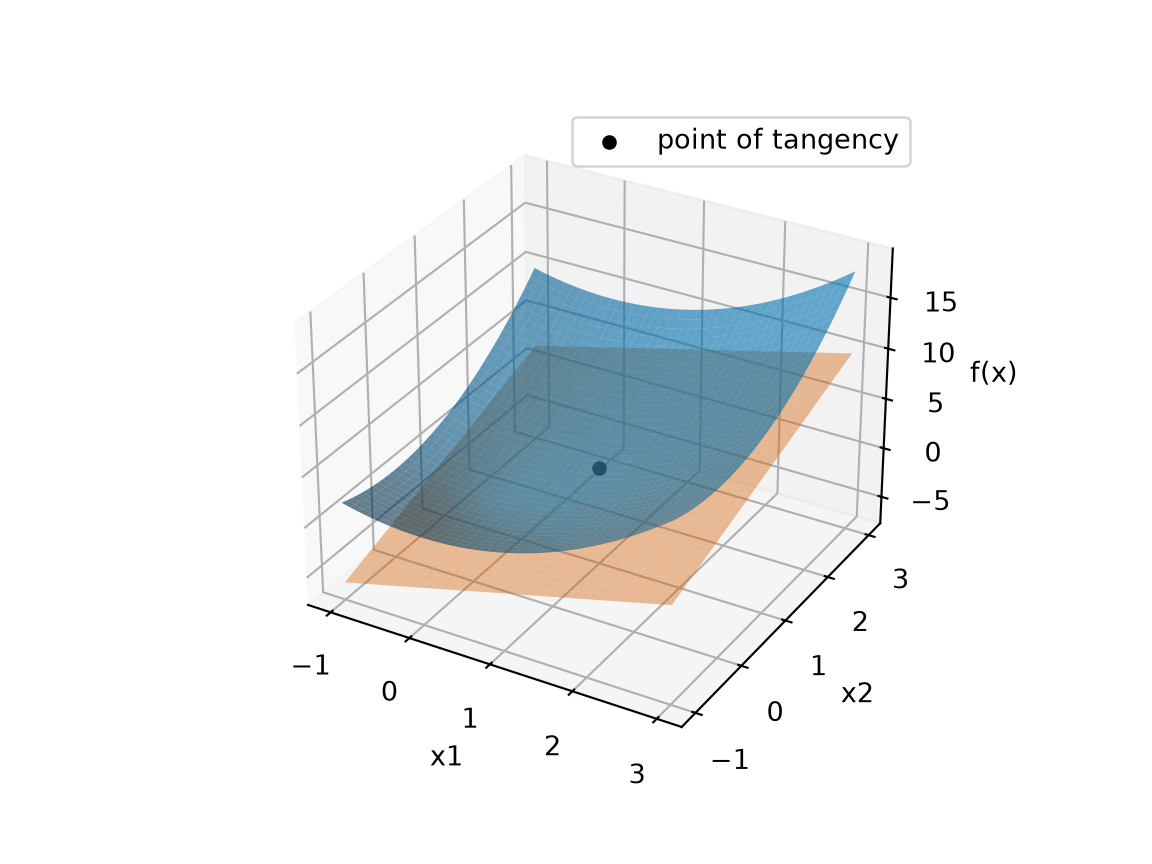
Figure 8: The tangent plane (vermilion) of the bowl \(f(\mathord{\smash[b]{\underset{\raise.3ex\hbox{$\scriptstyle\sim$}}{x}}\vphantom{x}}) = x_1^2 + x_2^2\) of Example 12 touches it at \({(1, 1)}^{\top}\) and lies below it.

• R
• Python

Remark 1 (The tangent plane in one variable). For \(p = 1\) the tangent plane is the tangent line \(s = f(y) + f'(y)\,(x - y)\), the line through \((y, f(y))\) with slope \(f'(y)\).

Theorem 5 (First-order characterization of convexity) Let \(f : \mathbb{R}^p \to \mathbb{R}\) have first partial derivatives that are continuous on \(\mathbb{R}^p\). Then \(f\) is convex if and only if

\[ f(\mathord{\smash[b]{\underset{\raise.3ex\hbox{$\scriptstyle\sim$}}{x}}\vphantom{x}}) \ge f(\mathord{\smash[b]{\underset{\raise.3ex\hbox{$\scriptstyle\sim$}}{y}}\vphantom{y}}) + {\mathopen{}\left(\frac{\partial}{\partial \mathord{\smash[b]{\underset{\raise.3ex\hbox{$\scriptstyle\sim$}}{x}}\vphantom{x}}} f(\mathord{\smash[b]{\underset{\raise.3ex\hbox{$\scriptstyle\sim$}}{y}}\vphantom{y}})\right)\mathclose{}}^{\top} (\mathord{\smash[b]{\underset{\raise.3ex\hbox{$\scriptstyle\sim$}}{x}}\vphantom{x}}- \mathord{\smash[b]{\underset{\raise.3ex\hbox{$\scriptstyle\sim$}}{y}}\vphantom{y}}) \qquad \text{for all } \mathord{\smash[b]{\underset{\raise.3ex\hbox{$\scriptstyle\sim$}}{x}}\vphantom{x}}, \mathord{\smash[b]{\underset{\raise.3ex\hbox{$\scriptstyle\sim$}}{y}}\vphantom{y}}\in \mathbb{R}^p: \tag{1}\]

every tangent plane (Definition 10) lies on or under the graph. If the inequality is strict whenever \(\mathord{\smash[b]{\underset{\raise.3ex\hbox{$\scriptstyle\sim$}}{x}}\vphantom{x}}\ne \mathord{\smash[b]{\underset{\raise.3ex\hbox{$\scriptstyle\sim$}}{y}}\vphantom{y}}\), then \(f\) is strictly convex (Definition 4).

Proof. Only if. Let \(\mathord{\smash[b]{\underset{\raise.3ex\hbox{$\scriptstyle\sim$}}{x}}\vphantom{x}}, \mathord{\smash[b]{\underset{\raise.3ex\hbox{$\scriptstyle\sim$}}{y}}\vphantom{y}}\in \mathbb{R}^p\), let \(\mathord{\smash[b]{\underset{\raise.3ex\hbox{$\scriptstyle\sim$}}{d}}\vphantom{d}} \stackrel{\text{def}}{=}\mathord{\smash[b]{\underset{\raise.3ex\hbox{$\scriptstyle\sim$}}{x}}\vphantom{x}}- \mathord{\smash[b]{\underset{\raise.3ex\hbox{$\scriptstyle\sim$}}{y}}\vphantom{y}}\), and let \(g(t) \stackrel{\text{def}}{=}f(\mathord{\smash[b]{\underset{\raise.3ex\hbox{$\scriptstyle\sim$}}{y}}\vphantom{y}}+ t \mathord{\smash[b]{\underset{\raise.3ex\hbox{$\scriptstyle\sim$}}{d}}\vphantom{d}})\). The inner function \(t \mapsto \mathord{\smash[b]{\underset{\raise.3ex\hbox{$\scriptstyle\sim$}}{y}}\vphantom{y}}+ t \mathord{\smash[b]{\underset{\raise.3ex\hbox{$\scriptstyle\sim$}}{d}}\vphantom{d}}\) has derivative \({\mathord{\smash[b]{\underset{\raise.3ex\hbox{$\scriptstyle\sim$}}{d}}\vphantom{d}}}^{\top}\), so the vector chain rule gives

\[ \begin{aligned} g'(0) &= {\mathord{\smash[b]{\underset{\raise.3ex\hbox{$\scriptstyle\sim$}}{d}}\vphantom{d}}}^{\top}\,\frac{\partial}{\partial \mathord{\smash[b]{\underset{\raise.3ex\hbox{$\scriptstyle\sim$}}{x}}\vphantom{x}}} f(\mathord{\smash[b]{\underset{\raise.3ex\hbox{$\scriptstyle\sim$}}{y}}\vphantom{y}}) && \text{(vector chain rule)} \\ &= {\mathopen{}\left(\frac{\partial}{\partial \mathord{\smash[b]{\underset{\raise.3ex\hbox{$\scriptstyle\sim$}}{x}}\vphantom{x}}} f(\mathord{\smash[b]{\underset{\raise.3ex\hbox{$\scriptstyle\sim$}}{y}}\vphantom{y}})\right)\mathclose{}}^{\top} \mathord{\smash[b]{\underset{\raise.3ex\hbox{$\scriptstyle\sim$}}{d}}\vphantom{d}}. && \text{(a } 1 \times 1 \text{ matrix equals its transpose)} \end{aligned} \]

For \(t \in (0, 1]\), \(\mathord{\smash[b]{\underset{\raise.3ex\hbox{$\scriptstyle\sim$}}{y}}\vphantom{y}}+ t \mathord{\smash[b]{\underset{\raise.3ex\hbox{$\scriptstyle\sim$}}{d}}\vphantom{d}} = t \mathord{\smash[b]{\underset{\raise.3ex\hbox{$\scriptstyle\sim$}}{x}}\vphantom{x}}+ (1 - t) \mathord{\smash[b]{\underset{\raise.3ex\hbox{$\scriptstyle\sim$}}{y}}\vphantom{y}}\), so

\[ \begin{aligned} g(t) - g(0) &= f(t \mathord{\smash[b]{\underset{\raise.3ex\hbox{$\scriptstyle\sim$}}{x}}\vphantom{x}}+ (1 - t) \mathord{\smash[b]{\underset{\raise.3ex\hbox{$\scriptstyle\sim$}}{y}}\vphantom{y}}) - f(\mathord{\smash[b]{\underset{\raise.3ex\hbox{$\scriptstyle\sim$}}{y}}\vphantom{y}}) && \text{(definition of } g \text{)} \\ &\le t f(\mathord{\smash[b]{\underset{\raise.3ex\hbox{$\scriptstyle\sim$}}{x}}\vphantom{x}}) + (1 - t) f(\mathord{\smash[b]{\underset{\raise.3ex\hbox{$\scriptstyle\sim$}}{y}}\vphantom{y}}) - f(\mathord{\smash[b]{\underset{\raise.3ex\hbox{$\scriptstyle\sim$}}{y}}\vphantom{y}}) && \text{(} f \text{ is convex)} \\ &= t\,(f(\mathord{\smash[b]{\underset{\raise.3ex\hbox{$\scriptstyle\sim$}}{x}}\vphantom{x}}) - f(\mathord{\smash[b]{\underset{\raise.3ex\hbox{$\scriptstyle\sim$}}{y}}\vphantom{y}})), && \text{(collect terms)} \end{aligned} \]

and dividing by \(t > 0\), \(\dfrac{g(t) - g(0)}{t} \le f(\mathord{\smash[b]{\underset{\raise.3ex\hbox{$\scriptstyle\sim$}}{x}}\vphantom{x}}) - f(\mathord{\smash[b]{\underset{\raise.3ex\hbox{$\scriptstyle\sim$}}{y}}\vphantom{y}})\). As \(t \to 0\) from the right, the left side tends to \(g'(0)\) (\(g\) is differentiable at \(0\), so the one-sided limit equals the two-sided derivative), and a limit of numbers that are all at most \(f(\mathord{\smash[b]{\underset{\raise.3ex\hbox{$\scriptstyle\sim$}}{x}}\vphantom{x}}) - f(\mathord{\smash[b]{\underset{\raise.3ex\hbox{$\scriptstyle\sim$}}{y}}\vphantom{y}})\) is at most \(f(\mathord{\smash[b]{\underset{\raise.3ex\hbox{$\scriptstyle\sim$}}{x}}\vphantom{x}}) - f(\mathord{\smash[b]{\underset{\raise.3ex\hbox{$\scriptstyle\sim$}}{y}}\vphantom{y}})\). So \({\mathopen{}\left(\frac{\partial}{\partial \mathord{\smash[b]{\underset{\raise.3ex\hbox{$\scriptstyle\sim$}}{x}}\vphantom{x}}} f(\mathord{\smash[b]{\underset{\raise.3ex\hbox{$\scriptstyle\sim$}}{y}}\vphantom{y}})\right)\mathclose{}}^{\top} (\mathord{\smash[b]{\underset{\raise.3ex\hbox{$\scriptstyle\sim$}}{x}}\vphantom{x}}- \mathord{\smash[b]{\underset{\raise.3ex\hbox{$\scriptstyle\sim$}}{y}}\vphantom{y}}) \le f(\mathord{\smash[b]{\underset{\raise.3ex\hbox{$\scriptstyle\sim$}}{x}}\vphantom{x}}) - f(\mathord{\smash[b]{\underset{\raise.3ex\hbox{$\scriptstyle\sim$}}{y}}\vphantom{y}})\), which rearranges to Equation 1.

If. Let \(\mathord{\smash[b]{\underset{\raise.3ex\hbox{$\scriptstyle\sim$}}{x}}\vphantom{x}}, \mathord{\smash[b]{\underset{\raise.3ex\hbox{$\scriptstyle\sim$}}{y}}\vphantom{y}}\in \mathbb{R}^p\), \(t \in [0, 1]\), \(\mathord{\smash[b]{\underset{\raise.3ex\hbox{$\scriptstyle\sim$}}{z}}\vphantom{z}} \stackrel{\text{def}}{=}t \mathord{\smash[b]{\underset{\raise.3ex\hbox{$\scriptstyle\sim$}}{x}}\vphantom{x}}+ (1 - t) \mathord{\smash[b]{\underset{\raise.3ex\hbox{$\scriptstyle\sim$}}{y}}\vphantom{y}}\), and \(\mathord{\smash[b]{\underset{\raise.3ex\hbox{$\scriptstyle\sim$}}{g}}\vphantom{g}} \stackrel{\text{def}}{=}\frac{\partial}{\partial \mathord{\smash[b]{\underset{\raise.3ex\hbox{$\scriptstyle\sim$}}{x}}\vphantom{x}}} f(\mathord{\smash[b]{\underset{\raise.3ex\hbox{$\scriptstyle\sim$}}{z}}\vphantom{z}})\). Applying Equation 1 at the point \(\mathord{\smash[b]{\underset{\raise.3ex\hbox{$\scriptstyle\sim$}}{z}}\vphantom{z}}\), once toward \(\mathord{\smash[b]{\underset{\raise.3ex\hbox{$\scriptstyle\sim$}}{x}}\vphantom{x}}\) and once toward \(\mathord{\smash[b]{\underset{\raise.3ex\hbox{$\scriptstyle\sim$}}{y}}\vphantom{y}}\),

\[ f(\mathord{\smash[b]{\underset{\raise.3ex\hbox{$\scriptstyle\sim$}}{x}}\vphantom{x}}) \ge f(\mathord{\smash[b]{\underset{\raise.3ex\hbox{$\scriptstyle\sim$}}{z}}\vphantom{z}}) + {\mathord{\smash[b]{\underset{\raise.3ex\hbox{$\scriptstyle\sim$}}{g}}\vphantom{g}}}^{\top} (\mathord{\smash[b]{\underset{\raise.3ex\hbox{$\scriptstyle\sim$}}{x}}\vphantom{x}}- \mathord{\smash[b]{\underset{\raise.3ex\hbox{$\scriptstyle\sim$}}{z}}\vphantom{z}}), \qquad f(\mathord{\smash[b]{\underset{\raise.3ex\hbox{$\scriptstyle\sim$}}{y}}\vphantom{y}}) \ge f(\mathord{\smash[b]{\underset{\raise.3ex\hbox{$\scriptstyle\sim$}}{z}}\vphantom{z}}) + {\mathord{\smash[b]{\underset{\raise.3ex\hbox{$\scriptstyle\sim$}}{g}}\vphantom{g}}}^{\top} (\mathord{\smash[b]{\underset{\raise.3ex\hbox{$\scriptstyle\sim$}}{y}}\vphantom{y}}- \mathord{\smash[b]{\underset{\raise.3ex\hbox{$\scriptstyle\sim$}}{z}}\vphantom{z}}). \]

Multiplying the first by \(t \ge 0\) and the second by \(1 - t \ge 0\) and adding,

\[ \begin{aligned} t f(\mathord{\smash[b]{\underset{\raise.3ex\hbox{$\scriptstyle\sim$}}{x}}\vphantom{x}}) + (1 - t) f(\mathord{\smash[b]{\underset{\raise.3ex\hbox{$\scriptstyle\sim$}}{y}}\vphantom{y}}) &\ge t \mathopen{}\left(f(\mathord{\smash[b]{\underset{\raise.3ex\hbox{$\scriptstyle\sim$}}{z}}\vphantom{z}}) + {\mathord{\smash[b]{\underset{\raise.3ex\hbox{$\scriptstyle\sim$}}{g}}\vphantom{g}}}^{\top} (\mathord{\smash[b]{\underset{\raise.3ex\hbox{$\scriptstyle\sim$}}{x}}\vphantom{x}}- \mathord{\smash[b]{\underset{\raise.3ex\hbox{$\scriptstyle\sim$}}{z}}\vphantom{z}})\right)\mathclose{} + (1 - t) \mathopen{}\left(f(\mathord{\smash[b]{\underset{\raise.3ex\hbox{$\scriptstyle\sim$}}{z}}\vphantom{z}}) + {\mathord{\smash[b]{\underset{\raise.3ex\hbox{$\scriptstyle\sim$}}{g}}\vphantom{g}}}^{\top} (\mathord{\smash[b]{\underset{\raise.3ex\hbox{$\scriptstyle\sim$}}{y}}\vphantom{y}}- \mathord{\smash[b]{\underset{\raise.3ex\hbox{$\scriptstyle\sim$}}{z}}\vphantom{z}})\right)\mathclose{} && \text{(multiply by } t, 1 - t \ge 0 \text{ and add)} \\ &= (t + (1 - t))\,f(\mathord{\smash[b]{\underset{\raise.3ex\hbox{$\scriptstyle\sim$}}{z}}\vphantom{z}}) + t\,{\mathord{\smash[b]{\underset{\raise.3ex\hbox{$\scriptstyle\sim$}}{g}}\vphantom{g}}}^{\top} (\mathord{\smash[b]{\underset{\raise.3ex\hbox{$\scriptstyle\sim$}}{x}}\vphantom{x}}- \mathord{\smash[b]{\underset{\raise.3ex\hbox{$\scriptstyle\sim$}}{z}}\vphantom{z}}) + (1 - t)\,{\mathord{\smash[b]{\underset{\raise.3ex\hbox{$\scriptstyle\sim$}}{g}}\vphantom{g}}}^{\top} (\mathord{\smash[b]{\underset{\raise.3ex\hbox{$\scriptstyle\sim$}}{y}}\vphantom{y}}- \mathord{\smash[b]{\underset{\raise.3ex\hbox{$\scriptstyle\sim$}}{z}}\vphantom{z}}) && \text{(distribute } t \text{ and } 1 - t \text{)} \\ &= f(\mathord{\smash[b]{\underset{\raise.3ex\hbox{$\scriptstyle\sim$}}{z}}\vphantom{z}}) + t\,{\mathord{\smash[b]{\underset{\raise.3ex\hbox{$\scriptstyle\sim$}}{g}}\vphantom{g}}}^{\top} (\mathord{\smash[b]{\underset{\raise.3ex\hbox{$\scriptstyle\sim$}}{x}}\vphantom{x}}- \mathord{\smash[b]{\underset{\raise.3ex\hbox{$\scriptstyle\sim$}}{z}}\vphantom{z}}) + (1 - t)\,{\mathord{\smash[b]{\underset{\raise.3ex\hbox{$\scriptstyle\sim$}}{g}}\vphantom{g}}}^{\top} (\mathord{\smash[b]{\underset{\raise.3ex\hbox{$\scriptstyle\sim$}}{y}}\vphantom{y}}- \mathord{\smash[b]{\underset{\raise.3ex\hbox{$\scriptstyle\sim$}}{z}}\vphantom{z}}) && \text{(} t + (1 - t) = 1 \text{)} \\ &= f(\mathord{\smash[b]{\underset{\raise.3ex\hbox{$\scriptstyle\sim$}}{z}}\vphantom{z}}) + {\mathord{\smash[b]{\underset{\raise.3ex\hbox{$\scriptstyle\sim$}}{g}}\vphantom{g}}}^{\top} \mathopen{}\left(t (\mathord{\smash[b]{\underset{\raise.3ex\hbox{$\scriptstyle\sim$}}{x}}\vphantom{x}}- \mathord{\smash[b]{\underset{\raise.3ex\hbox{$\scriptstyle\sim$}}{z}}\vphantom{z}}) + (1 - t) (\mathord{\smash[b]{\underset{\raise.3ex\hbox{$\scriptstyle\sim$}}{y}}\vphantom{y}}- \mathord{\smash[b]{\underset{\raise.3ex\hbox{$\scriptstyle\sim$}}{z}}\vphantom{z}})\right)\mathclose{} && \text{(factor out } {\mathord{\smash[b]{\underset{\raise.3ex\hbox{$\scriptstyle\sim$}}{g}}\vphantom{g}}}^{\top} \text{; matrix products distribute)} \\ &= f(\mathord{\smash[b]{\underset{\raise.3ex\hbox{$\scriptstyle\sim$}}{z}}\vphantom{z}}) + {\mathord{\smash[b]{\underset{\raise.3ex\hbox{$\scriptstyle\sim$}}{g}}\vphantom{g}}}^{\top} \mathopen{}\left(t \mathord{\smash[b]{\underset{\raise.3ex\hbox{$\scriptstyle\sim$}}{x}}\vphantom{x}}+ (1 - t) \mathord{\smash[b]{\underset{\raise.3ex\hbox{$\scriptstyle\sim$}}{y}}\vphantom{y}}- \mathord{\smash[b]{\underset{\raise.3ex\hbox{$\scriptstyle\sim$}}{z}}\vphantom{z}}\right)\mathclose{} && \text{(collect terms)} \\ &= f(\mathord{\smash[b]{\underset{\raise.3ex\hbox{$\scriptstyle\sim$}}{z}}\vphantom{z}}). && \text{(definition of } \mathord{\smash[b]{\underset{\raise.3ex\hbox{$\scriptstyle\sim$}}{z}}\vphantom{z}} \text{)} \end{aligned} \]

That inequality is the defining inequality of a convex function. If Equation 1 is strict for distinct points, and \(\mathord{\smash[b]{\underset{\raise.3ex\hbox{$\scriptstyle\sim$}}{x}}\vphantom{x}}\ne \mathord{\smash[b]{\underset{\raise.3ex\hbox{$\scriptstyle\sim$}}{y}}\vphantom{y}}\) and \(t \in (0, 1)\), then:

• \(\mathord{\smash[b]{\underset{\raise.3ex\hbox{$\scriptstyle\sim$}}{z}}\vphantom{z}}\) differs from both \(\mathord{\smash[b]{\underset{\raise.3ex\hbox{$\scriptstyle\sim$}}{x}}\vphantom{x}}\) and \(\mathord{\smash[b]{\underset{\raise.3ex\hbox{$\scriptstyle\sim$}}{y}}\vphantom{y}}\), since \(\mathord{\smash[b]{\underset{\raise.3ex\hbox{$\scriptstyle\sim$}}{x}}\vphantom{x}}- \mathord{\smash[b]{\underset{\raise.3ex\hbox{$\scriptstyle\sim$}}{z}}\vphantom{z}} = (1 - t)(\mathord{\smash[b]{\underset{\raise.3ex\hbox{$\scriptstyle\sim$}}{x}}\vphantom{x}}- \mathord{\smash[b]{\underset{\raise.3ex\hbox{$\scriptstyle\sim$}}{y}}\vphantom{y}}) \ne \mathord{\smash[b]{\underset{\raise.3ex\hbox{$\scriptstyle\sim$}}{0}}\vphantom{0}}\) and \(\mathord{\smash[b]{\underset{\raise.3ex\hbox{$\scriptstyle\sim$}}{y}}\vphantom{y}}- \mathord{\smash[b]{\underset{\raise.3ex\hbox{$\scriptstyle\sim$}}{z}}\vphantom{z}} = t (\mathord{\smash[b]{\underset{\raise.3ex\hbox{$\scriptstyle\sim$}}{y}}\vphantom{y}}- \mathord{\smash[b]{\underset{\raise.3ex\hbox{$\scriptstyle\sim$}}{x}}\vphantom{x}}) \ne \mathord{\smash[b]{\underset{\raise.3ex\hbox{$\scriptstyle\sim$}}{0}}\vphantom{0}}\);
• so both inequalities at \(\mathord{\smash[b]{\underset{\raise.3ex\hbox{$\scriptstyle\sim$}}{z}}\vphantom{z}}\) are strict;
• both multipliers \(t\) and \(1 - t\) are positive, so the first step of the display is strict, and \(f\) is strictly convex.

Example 13 (Tangent lines under a parabola) For \(f(x) = x^2\), the right side of Equation 1 is \(y^2 + 2y (x - y) = 2xy - y^2\), and

\[ \begin{aligned} f(x) - (2xy - y^2) &= x^2 - 2xy + y^2 \\ &= (x - y)^2 \\ &\ge 0, \end{aligned} \]

with equality only at \(x = y\), confirming that \(x^2\) is strictly convex. For \(g(x) = -x^2\) the inequality fails: at \(y = 0\) the tangent line is \(s = 0\), and \(g(1) = -1 < 0\).

tl_x_ft <- seq(-1, 3, length.out = 201)
tl_curve_ft <- tibble::tibble(x = tl_x_ft, s = tl_x_ft^2)
tl_line_ft <- tibble::tibble(x = tl_x_ft, s = 2 * tl_x_ft - 1)
tl_point_ft <- tibble::tibble(x = 1, s = 1)
tl_aes_ft <- ggplot2::aes(x, s)
ggplot2::ggplot(tl_curve_ft, tl_aes_ft) +
  ggplot2::geom_line(colour = "#0072B2") +
  ggplot2::geom_line(
    data = tl_line_ft, colour = "#D55E00", linetype = "dashed"
  ) +
  ggplot2::geom_point(data = tl_point_ft, colour = "#D55E00", size = 3) +
  ggplot2::labs(x = "x", y = "s")

import matplotlib.pyplot as plt
import numpy as np

tl_x_ft = np.linspace(-1, 3, 201)
fig, ax = plt.subplots(figsize=(5, 4), layout="constrained")
ax.plot(tl_x_ft, tl_x_ft**2, color="#0072B2", label="f(x) = x^2")
ax.plot(tl_x_ft, 2 * tl_x_ft - 1, "--", color="#D55E00",
        label="tangent line at 1")
ax.plot(1, 1, "o", color="#D55E00", markersize=8)
ax.set_xlabel("x")
ax.set_ylabel("s")
ax.legend(loc="upper center")
plt.show()

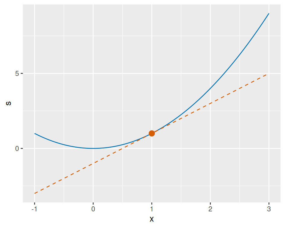
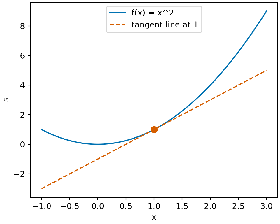
Figure 9: The tangent line \(s = 2x - 1\) of \(f(x) = x^2\) at \(y = 1\) (Example 12). It touches the graph at \((1, 1)\) and lies below it everywhere else, as in Example 13.

• R
• Python

Theorem 6 (Second-derivative test for convexity) Let \(f : \mathbb{R}^p \to \mathbb{R}\) have first and second partial derivatives that are continuous on \(\mathbb{R}^p\).

1. If \(\mathbf{H}_f(\mathord{\smash[b]{\underset{\raise.3ex\hbox{$\scriptstyle\sim$}}{x}}\vphantom{x}})\) is positive semidefinite for every \(\mathord{\smash[b]{\underset{\raise.3ex\hbox{$\scriptstyle\sim$}}{x}}\vphantom{x}}\), then \(f\) is convex.
2. If \(\mathbf{H}_f(\mathord{\smash[b]{\underset{\raise.3ex\hbox{$\scriptstyle\sim$}}{x}}\vphantom{x}})\) is positive definite for every \(\mathord{\smash[b]{\underset{\raise.3ex\hbox{$\scriptstyle\sim$}}{x}}\vphantom{x}}\), then \(f\) is strictly convex (Definition 4).

Proof. Let \(\mathord{\smash[b]{\underset{\raise.3ex\hbox{$\scriptstyle\sim$}}{x}}\vphantom{x}}, \mathord{\smash[b]{\underset{\raise.3ex\hbox{$\scriptstyle\sim$}}{y}}\vphantom{y}}\in \mathbb{R}^p\). By Theorem 6 in Critical Points and Optimality Conditions with \(\mathord{\smash[b]{\underset{\raise.3ex\hbox{$\scriptstyle\sim$}}{z}}\vphantom{z}} = \mathord{\smash[b]{\underset{\raise.3ex\hbox{$\scriptstyle\sim$}}{y}}\vphantom{y}}\) and \(\mathord{\smash[b]{\underset{\raise.3ex\hbox{$\scriptstyle\sim$}}{h}}\vphantom{h}} = \mathord{\smash[b]{\underset{\raise.3ex\hbox{$\scriptstyle\sim$}}{x}}\vphantom{x}}- \mathord{\smash[b]{\underset{\raise.3ex\hbox{$\scriptstyle\sim$}}{y}}\vphantom{y}}\), there is a \(\tau\in (0, 1)\) such that, with \(\mathord{\smash[b]{\underset{\raise.3ex\hbox{$\scriptstyle\sim$}}{w}}\vphantom{w}} \stackrel{\text{def}}{=}\mathord{\smash[b]{\underset{\raise.3ex\hbox{$\scriptstyle\sim$}}{y}}\vphantom{y}}+ \tau(\mathord{\smash[b]{\underset{\raise.3ex\hbox{$\scriptstyle\sim$}}{x}}\vphantom{x}}- \mathord{\smash[b]{\underset{\raise.3ex\hbox{$\scriptstyle\sim$}}{y}}\vphantom{y}})\),

\[ \begin{aligned} f(\mathord{\smash[b]{\underset{\raise.3ex\hbox{$\scriptstyle\sim$}}{x}}\vphantom{x}}) &= f(\mathord{\smash[b]{\underset{\raise.3ex\hbox{$\scriptstyle\sim$}}{y}}\vphantom{y}}) + {\mathopen{}\left(\frac{\partial}{\partial \mathord{\smash[b]{\underset{\raise.3ex\hbox{$\scriptstyle\sim$}}{x}}\vphantom{x}}} f(\mathord{\smash[b]{\underset{\raise.3ex\hbox{$\scriptstyle\sim$}}{y}}\vphantom{y}})\right)\mathclose{}}^{\top} (\mathord{\smash[b]{\underset{\raise.3ex\hbox{$\scriptstyle\sim$}}{x}}\vphantom{x}}- \mathord{\smash[b]{\underset{\raise.3ex\hbox{$\scriptstyle\sim$}}{y}}\vphantom{y}}) + \frac{1}{2}\,{(\mathord{\smash[b]{\underset{\raise.3ex\hbox{$\scriptstyle\sim$}}{x}}\vphantom{x}}- \mathord{\smash[b]{\underset{\raise.3ex\hbox{$\scriptstyle\sim$}}{y}}\vphantom{y}})}^{\top}\,\mathbf{H}_f(\mathord{\smash[b]{\underset{\raise.3ex\hbox{$\scriptstyle\sim$}}{w}}\vphantom{w}})\,(\mathord{\smash[b]{\underset{\raise.3ex\hbox{$\scriptstyle\sim$}}{x}}\vphantom{x}}- \mathord{\smash[b]{\underset{\raise.3ex\hbox{$\scriptstyle\sim$}}{y}}\vphantom{y}}) && \text{(}\href{optimization-critical-points.qmd#thm-taylor-mv}{\text{Theorem~6 in Critical Points and Optimality Conditions}}\text{)} \\ &\ge f(\mathord{\smash[b]{\underset{\raise.3ex\hbox{$\scriptstyle\sim$}}{y}}\vphantom{y}}) + {\mathopen{}\left(\frac{\partial}{\partial \mathord{\smash[b]{\underset{\raise.3ex\hbox{$\scriptstyle\sim$}}{x}}\vphantom{x}}} f(\mathord{\smash[b]{\underset{\raise.3ex\hbox{$\scriptstyle\sim$}}{y}}\vphantom{y}})\right)\mathclose{}}^{\top} (\mathord{\smash[b]{\underset{\raise.3ex\hbox{$\scriptstyle\sim$}}{x}}\vphantom{x}}- \mathord{\smash[b]{\underset{\raise.3ex\hbox{$\scriptstyle\sim$}}{y}}\vphantom{y}}). && \text{(} \mathbf{H}_f(\mathord{\smash[b]{\underset{\raise.3ex\hbox{$\scriptstyle\sim$}}{w}}\vphantom{w}}) \text{ is positive semidefinite)} \end{aligned} \]

This inequality is Equation 1, so \(f\) is convex by Theorem 5. Under the hypothesis of part 2 and with \(\mathord{\smash[b]{\underset{\raise.3ex\hbox{$\scriptstyle\sim$}}{x}}\vphantom{x}}\ne \mathord{\smash[b]{\underset{\raise.3ex\hbox{$\scriptstyle\sim$}}{y}}\vphantom{y}}\), the quadratic-form term is positive, so the inequality is strict, and \(f\) is strictly convex by the last sentence of Theorem 5.

Example 14 (Using the Hessian to show convexity)  

• For a symmetric positive semidefinite \(\mathbf{A}\), \(f(\mathord{\smash[b]{\underset{\raise.3ex\hbox{$\scriptstyle\sim$}}{x}}\vphantom{x}}) = {\mathord{\smash[b]{\underset{\raise.3ex\hbox{$\scriptstyle\sim$}}{x}}\vphantom{x}}}^{\top} \mathbf{A} \mathord{\smash[b]{\underset{\raise.3ex\hbox{$\scriptstyle\sim$}}{x}}\vphantom{x}}\) has Hessian \(2 \mathbf{A}\) (by the Hessian of a quadratic form), which is positive semidefinite because \({\mathord{\smash[b]{\underset{\raise.3ex\hbox{$\scriptstyle\sim$}}{h}}\vphantom{h}}}^{\top} (2 \mathbf{A}) \mathord{\smash[b]{\underset{\raise.3ex\hbox{$\scriptstyle\sim$}}{h}}\vphantom{h}} = 2\,{\mathord{\smash[b]{\underset{\raise.3ex\hbox{$\scriptstyle\sim$}}{h}}\vphantom{h}}}^{\top} \mathbf{A} \mathord{\smash[b]{\underset{\raise.3ex\hbox{$\scriptstyle\sim$}}{h}}\vphantom{h}} \ge 0\); so \(f\) is convex.

• \(f(\mathord{\smash[b]{\underset{\raise.3ex\hbox{$\scriptstyle\sim$}}{x}}\vphantom{x}}) = x_1^2 + x_2^2 - 2 x_1\) has Hessian \(2 \mathbf{I}_2\) (Example 16 in Critical Points and Optimality Conditions), which is positive definite, so \(f\) is strictly convex.

• \(f(\mathord{\smash[b]{\underset{\raise.3ex\hbox{$\scriptstyle\sim$}}{x}}\vphantom{x}}) = e^{2x_1 + x_2} - x_1\) has Hessian \(e^{u} \begin{bmatrix} 4 & 2 \\ 2 & 1 \end{bmatrix}\) with \(u = 2x_1 + x_2\) (the Hessian example), and

  \[ \begin{aligned} {\mathord{\smash[b]{\underset{\raise.3ex\hbox{$\scriptstyle\sim$}}{h}}\vphantom{h}}}^{\top}\,\mathbf{H}_f(\mathord{\smash[b]{\underset{\raise.3ex\hbox{$\scriptstyle\sim$}}{x}}\vphantom{x}})\,\mathord{\smash[b]{\underset{\raise.3ex\hbox{$\scriptstyle\sim$}}{h}}\vphantom{h}} &= e^{u} (4 h_1^2 + 4 h_1 h_2 + h_2^2) \\ &= e^{u} (2 h_1 + h_2)^2 \\ &\ge 0, \end{aligned} \]

  so \(f\) is convex. The Hessian is not positive definite (\(\mathord{\smash[b]{\underset{\raise.3ex\hbox{$\scriptstyle\sim$}}{h}}\vphantom{h}} = {(1, -2)}^{\top}\) gives \(0\)), so part 2 does not apply, and in fact \(f\) is not strictly convex: along \(\mathord{\smash[b]{\underset{\raise.3ex\hbox{$\scriptstyle\sim$}}{x}}\vphantom{x}}= t\,{(1, -2)}^{\top}\),

  \[ \begin{aligned} u &= 2t - 2t \\ &= 0 \end{aligned} \]

  and \(f = 1 - t\) is linear in \(t\), so the convexity inequality holds with equality there.

ch_x1_ch <- seq(-1, 1, length.out = 101)
ch_x2_ch <- seq(-3, 3, length.out = 101)
ch_grid_ch <- tidyr::expand_grid(x1 = ch_x1_ch, x2 = ch_x2_ch)
ch_u_ch <- 2 * ch_grid_ch$x1 + ch_grid_ch$x2
ch_grid_ch$z <- exp(ch_u_ch) - ch_grid_ch$x1
ch_line_x1_ch <- c(-1, 1)
ch_line_x2_ch <- c(2, -2)
ch_line_ch <- tibble::tibble(x1 = ch_line_x1_ch, x2 = ch_line_x2_ch)
ch_aes_ch <- ggplot2::aes(x1, x2)
ch_z_aes_ch <- ggplot2::aes(z = z)
ggplot2::ggplot(ch_grid_ch, ch_aes_ch) +
  ggplot2::geom_contour(ch_z_aes_ch, colour = "#0072B2", bins = 12) +
  ggplot2::geom_line(
    data = ch_line_ch, colour = "#D55E00", linetype = "dashed"
  ) +
  ggplot2::labs(x = "x1", y = "x2")

import matplotlib.pyplot as plt
import numpy as np

ch_x1_ax = np.linspace(-1, 1, 101)
ch_x2_ax = np.linspace(-3, 3, 101)
ch_xx_ax, ch_yy_ax = np.meshgrid(ch_x1_ax, ch_x2_ax)
ch_z_ax = np.exp(2 * ch_xx_ax + ch_yy_ax) - ch_xx_ax
fig, ax = plt.subplots(figsize=(5, 4), layout="constrained")
ax.contour(ch_xx_ax, ch_yy_ax, ch_z_ax, levels=12, colors="#0072B2")
ax.plot([-1, 1], [2, -2], "--", color="#D55E00")
ax.set_xlabel("x1")
ax.set_ylabel("x2")
plt.show();

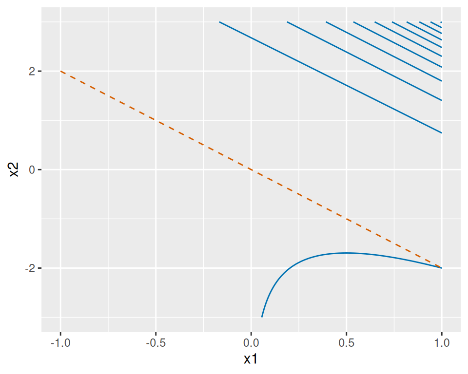
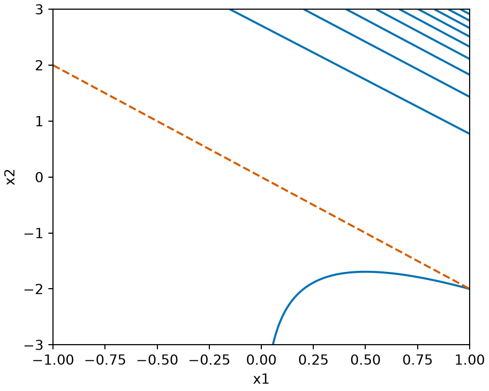
Figure 10: Level curves of the third function in Example 14. Along the dashed line through the origin in the direction \({(1, -2)}^{\top}\) the function is linear, so the function is convex but not strictly convex.

• R
• Python

ch_x1_sf <- seq(-1, 1, length.out = 101)
ch_x2_sf <- seq(-3, 3, length.out = 101)
ch_grid_sf <- tidyr::expand_grid(x1 = ch_x1_sf, x2 = ch_x2_sf)
ch_u_sf <- 2 * ch_grid_sf$x1 + ch_grid_sf$x2
ch_value_sf <- exp(ch_u_sf) - ch_grid_sf$x1
ch_n2_sf <- length(ch_x2_sf)
ch_z_sf <- matrix(ch_value_sf, nrow = ch_n2_sf)
ch_l_x1_sf <- seq(-1, 1, length.out = 21)
ch_line_sf <- tibble::tibble(x1 = ch_l_x1_sf)
ch_line_sf$x2 <- -2 * ch_line_sf$x1
ch_lu_sf <- 2 * ch_line_sf$x1 + ch_line_sf$x2
ch_line_sf$z <- exp(ch_lu_sf) - ch_line_sf$x1
ch_dash_sf <- list(color = "#D55E00", dash = "dash", width = 5)
ch_stops_sf <- c(0, 1)
ch_cols_sf <- c("#CCE0F0", "#0072B2")
ch_scale_sf <- list(ch_stops_sf, ch_cols_sf)
ch_eye_sf <- list(x = 1.6, y = -1.6, z = 0.9)
ch_camera_sf <- list(eye = ch_eye_sf)
ch_xaxis_sf <- list(title = "x1")
ch_yaxis_sf <- list(title = "x2")
ch_zaxis_sf <- list(title = "f(x)")
ch_scene_sf <- list(
  xaxis = ch_xaxis_sf,
  yaxis = ch_yaxis_sf,
  zaxis = ch_zaxis_sf,
  camera = ch_camera_sf
)
ch_legend_sf <- list(orientation = "h")
plotly::plot_ly() |>
  plotly::add_surface(
    x = ch_x1_sf,
    y = ch_x2_sf,
    z = ch_z_sf,
    colorscale = ch_scale_sf,
    showscale = FALSE,
    opacity = 0.8
  ) |>
  plotly::add_trace(
    data = ch_line_sf,
    x = ~x1,
    y = ~x2,
    z = ~z,
    type = "scatter3d",
    mode = "lines",
    line = ch_dash_sf,
    name = "f is linear"
  ) |>
  plotly::layout(scene = ch_scene_sf, legend = ch_legend_sf)

import html
import numpy as np
import plotly.graph_objects as go

fig_alt = (
    "Surface plot of f(x) = exp(2 x1 + x2) - x1 for x1 from -1 to 1 and x2 from "
    "-3 to 3. The surface is a trough that rises steeply toward the upper "
    "right, where 2 x1 plus x2 is large, and is nearly flat on the lower left. "
    "A dashed vermilion straight line along the direction (1, -2) through the "
    "origin lies on the surface, because f is linear there."
)

ch_x1_3d = np.linspace(-1, 1, 101)
ch_x2_3d = np.linspace(-3, 3, 101)
ch_xx_3d, ch_yy_3d = np.meshgrid(ch_x1_3d, ch_x2_3d)
ch_z_3d = np.exp(2 * ch_xx_3d + ch_yy_3d) - ch_xx_3d
ch_line_x1_3d = np.linspace(-1, 1, 21)
ch_line_x2_3d = -2 * ch_line_x1_3d
ch_line_z_3d = np.exp(2 * ch_line_x1_3d + ch_line_x2_3d) - ch_line_x1_3d
fig = go.Figure(data=[
    go.Surface(
        x=ch_x1_3d,
        y=ch_x2_3d,
        z=ch_z_3d,
        colorscale=[[0, "#CCE0F0"], [1, "#0072B2"]],
        showscale=False,
        opacity=0.6,
        showlegend=False,
    ),
    go.Scatter3d(x=ch_line_x1_3d, y=ch_line_x2_3d, z=ch_line_z_3d,
                 mode="lines",
                 line=dict(color="#D55E00", width=5, dash="dash"),
                 name="f is linear"),
])
fig.update_layout(
    scene=dict(
        xaxis_title="x1",
        yaxis_title="x2",
        zaxis_title="f(x)",
        camera=dict(eye=dict(x=1.6, y=-1.6, z=0.9)),
    ),
    legend=dict(orientation="h"),
);
print(
    "```{=html}\n"
    + f'<div role="img" aria-label="{html.escape(fig_alt)}">\n'
    + fig.to_html(full_html=False, include_plotlyjs="cdn")
    + "\n</div>\n```"
)

Figure 11: The graph of the third function in Example 14, the surface whose level curves are in Figure 10. Along the dashed line through the origin in the direction \({(1, -2)}^{\top}\) the surface is a straight line, so the function is linear there. The function is therefore convex but not strictly convex.

• R
• Python

Example 15 (Strictly convex with a singular Hessian) Part 2 is sufficient but not necessary. \(f(x) = x^4\) has

\[ \begin{aligned} f''(0) &= 12 \cdot 0^2 \\ &= 0, \end{aligned} \]

so \(\mathbf{H}_f(0) = [0]\) is singular and not positive definite. Yet \(f\) is strictly convex, by the strict form of Equation 1: for \(x \ne y\),

\[ \begin{aligned} x^4 - y^4 - 4 y^3 (x - y) &= (x - y)(x^3 + x^2 y + x y^2 + y^3) - 4 y^3 (x - y) && \text{(factor } x^4 - y^4 \text{)} \\ &= (x - y)(x^3 + x^2 y + x y^2 - 3 y^3) && \text{(collect the } y^3 \text{ terms)} \\ &= (x - y)^2 (x^2 + 2 x y + 3 y^2) && \text{(} (x - y)(x^2 + 2 x y + 3 y^2) = x^3 + x^2 y + x y^2 - 3 y^3 \text{)} \\ &= (x - y)^2 \mathopen{}\left((x + y)^2 + 2 y^2\right)\mathclose{}, && \text{(complete the square)} \end{aligned} \]

which is positive: \((x - y)^2 > 0\), and \((x + y)^2 + 2 y^2 = 0\) would need \(y = 0\) and then

\[ \begin{aligned} x &= 0 \\ &= y. \end{aligned} \]

Theorem 7 (A convex function has a positive semidefinite Hessian) Let \(f : \mathbb{R}^p \to \mathbb{R}\) have first and second partial derivatives that are continuous on \(\mathbb{R}^p\). If \(f\) is convex, then the Hessian \(\mathbf{H}_f(\mathord{\smash[b]{\underset{\raise.3ex\hbox{$\scriptstyle\sim$}}{x}}\vphantom{x}})\) is positive semidefinite for every \(\mathord{\smash[b]{\underset{\raise.3ex\hbox{$\scriptstyle\sim$}}{x}}\vphantom{x}}\in \mathbb{R}^p\).

Proof. Fix \(\mathord{\smash[b]{\underset{\raise.3ex\hbox{$\scriptstyle\sim$}}{x}}\vphantom{x}}, \mathord{\smash[b]{\underset{\raise.3ex\hbox{$\scriptstyle\sim$}}{v}}\vphantom{v}} \in \mathbb{R}^p\). Let \(h > 0\). By Theorem 6 in Critical Points and Optimality Conditions applied with \(\mathord{\smash[b]{\underset{\raise.3ex\hbox{$\scriptstyle\sim$}}{z}}\vphantom{z}} = \mathord{\smash[b]{\underset{\raise.3ex\hbox{$\scriptstyle\sim$}}{x}}\vphantom{x}}\) and \(\mathord{\smash[b]{\underset{\raise.3ex\hbox{$\scriptstyle\sim$}}{h}}\vphantom{h}} = h\mathord{\smash[b]{\underset{\raise.3ex\hbox{$\scriptstyle\sim$}}{v}}\vphantom{v}}\), and again with \(\mathord{\smash[b]{\underset{\raise.3ex\hbox{$\scriptstyle\sim$}}{h}}\vphantom{h}} = -h\mathord{\smash[b]{\underset{\raise.3ex\hbox{$\scriptstyle\sim$}}{v}}\vphantom{v}}\), there are \(\tau_+, \tau_- \in (0, 1)\) with

\[ \begin{aligned} f(\mathord{\smash[b]{\underset{\raise.3ex\hbox{$\scriptstyle\sim$}}{x}}\vphantom{x}}+ h\mathord{\smash[b]{\underset{\raise.3ex\hbox{$\scriptstyle\sim$}}{v}}\vphantom{v}}) &= f(\mathord{\smash[b]{\underset{\raise.3ex\hbox{$\scriptstyle\sim$}}{x}}\vphantom{x}}) + h\,{\mathopen{}\left(\frac{\partial}{\partial \mathord{\smash[b]{\underset{\raise.3ex\hbox{$\scriptstyle\sim$}}{x}}\vphantom{x}}} f(\mathord{\smash[b]{\underset{\raise.3ex\hbox{$\scriptstyle\sim$}}{x}}\vphantom{x}})\right)\mathclose{}}^{\top} \mathord{\smash[b]{\underset{\raise.3ex\hbox{$\scriptstyle\sim$}}{v}}\vphantom{v}} + \frac{h^2}{2}\,{\mathord{\smash[b]{\underset{\raise.3ex\hbox{$\scriptstyle\sim$}}{v}}\vphantom{v}}}^{\top}\,\mathbf{H}_f(\mathord{\smash[b]{\underset{\raise.3ex\hbox{$\scriptstyle\sim$}}{w}}\vphantom{w}}_+)\,\mathord{\smash[b]{\underset{\raise.3ex\hbox{$\scriptstyle\sim$}}{v}}\vphantom{v}} && \text{(}\href{optimization-critical-points.qmd#thm-taylor-mv}{\text{Theorem~6 in Critical Points and Optimality Conditions}}\text{)} \\ f(\mathord{\smash[b]{\underset{\raise.3ex\hbox{$\scriptstyle\sim$}}{x}}\vphantom{x}}- h\mathord{\smash[b]{\underset{\raise.3ex\hbox{$\scriptstyle\sim$}}{v}}\vphantom{v}}) &= f(\mathord{\smash[b]{\underset{\raise.3ex\hbox{$\scriptstyle\sim$}}{x}}\vphantom{x}}) - h\,{\mathopen{}\left(\frac{\partial}{\partial \mathord{\smash[b]{\underset{\raise.3ex\hbox{$\scriptstyle\sim$}}{x}}\vphantom{x}}} f(\mathord{\smash[b]{\underset{\raise.3ex\hbox{$\scriptstyle\sim$}}{x}}\vphantom{x}})\right)\mathclose{}}^{\top} \mathord{\smash[b]{\underset{\raise.3ex\hbox{$\scriptstyle\sim$}}{v}}\vphantom{v}} + \frac{h^2}{2}\,{\mathord{\smash[b]{\underset{\raise.3ex\hbox{$\scriptstyle\sim$}}{v}}\vphantom{v}}}^{\top}\,\mathbf{H}_f(\mathord{\smash[b]{\underset{\raise.3ex\hbox{$\scriptstyle\sim$}}{w}}\vphantom{w}}_-)\,\mathord{\smash[b]{\underset{\raise.3ex\hbox{$\scriptstyle\sim$}}{v}}\vphantom{v}}, && \text{(}\href{optimization-critical-points.qmd#thm-taylor-mv}{\text{Theorem~6 in Critical Points and Optimality Conditions}}\text{)} \end{aligned} \]

where \(\mathord{\smash[b]{\underset{\raise.3ex\hbox{$\scriptstyle\sim$}}{w}}\vphantom{w}}_\pm = \mathord{\smash[b]{\underset{\raise.3ex\hbox{$\scriptstyle\sim$}}{x}}\vphantom{x}}\pm \tau_\pm h\mathord{\smash[b]{\underset{\raise.3ex\hbox{$\scriptstyle\sim$}}{v}}\vphantom{v}}\). Adding the two equations cancels the first-order summands:

\[ f(\mathord{\smash[b]{\underset{\raise.3ex\hbox{$\scriptstyle\sim$}}{x}}\vphantom{x}}+ h\mathord{\smash[b]{\underset{\raise.3ex\hbox{$\scriptstyle\sim$}}{v}}\vphantom{v}}) + f(\mathord{\smash[b]{\underset{\raise.3ex\hbox{$\scriptstyle\sim$}}{x}}\vphantom{x}}- h\mathord{\smash[b]{\underset{\raise.3ex\hbox{$\scriptstyle\sim$}}{v}}\vphantom{v}}) - 2 f(\mathord{\smash[b]{\underset{\raise.3ex\hbox{$\scriptstyle\sim$}}{x}}\vphantom{x}}) = \frac{h^2}{2}\,{\mathord{\smash[b]{\underset{\raise.3ex\hbox{$\scriptstyle\sim$}}{v}}\vphantom{v}}}^{\top}\mathopen{}\left(\mathbf{H}_f(\mathord{\smash[b]{\underset{\raise.3ex\hbox{$\scriptstyle\sim$}}{w}}\vphantom{w}}_+) + \mathbf{H}_f(\mathord{\smash[b]{\underset{\raise.3ex\hbox{$\scriptstyle\sim$}}{w}}\vphantom{w}}_-)\right)\mathclose{}\mathord{\smash[b]{\underset{\raise.3ex\hbox{$\scriptstyle\sim$}}{v}}\vphantom{v}}. \]

Since \(f\) is convex and \(\mathord{\smash[b]{\underset{\raise.3ex\hbox{$\scriptstyle\sim$}}{x}}\vphantom{x}}= \frac{1}{2}(\mathord{\smash[b]{\underset{\raise.3ex\hbox{$\scriptstyle\sim$}}{x}}\vphantom{x}}+ h\mathord{\smash[b]{\underset{\raise.3ex\hbox{$\scriptstyle\sim$}}{v}}\vphantom{v}}) + \frac{1}{2}(\mathord{\smash[b]{\underset{\raise.3ex\hbox{$\scriptstyle\sim$}}{x}}\vphantom{x}}- h\mathord{\smash[b]{\underset{\raise.3ex\hbox{$\scriptstyle\sim$}}{v}}\vphantom{v}})\),

\[ f(\mathord{\smash[b]{\underset{\raise.3ex\hbox{$\scriptstyle\sim$}}{x}}\vphantom{x}}) \le \frac{1}{2} f(\mathord{\smash[b]{\underset{\raise.3ex\hbox{$\scriptstyle\sim$}}{x}}\vphantom{x}}+ h\mathord{\smash[b]{\underset{\raise.3ex\hbox{$\scriptstyle\sim$}}{v}}\vphantom{v}}) + \frac{1}{2} f(\mathord{\smash[b]{\underset{\raise.3ex\hbox{$\scriptstyle\sim$}}{x}}\vphantom{x}}- h\mathord{\smash[b]{\underset{\raise.3ex\hbox{$\scriptstyle\sim$}}{v}}\vphantom{v}}), \]

so the left side of the previous display is nonnegative. Dividing by \(h^2 / 2\) gives

\[ {\mathord{\smash[b]{\underset{\raise.3ex\hbox{$\scriptstyle\sim$}}{v}}\vphantom{v}}}^{\top}\mathopen{}\left(\mathbf{H}_f(\mathord{\smash[b]{\underset{\raise.3ex\hbox{$\scriptstyle\sim$}}{w}}\vphantom{w}}_+) + \mathbf{H}_f(\mathord{\smash[b]{\underset{\raise.3ex\hbox{$\scriptstyle\sim$}}{w}}\vphantom{w}}_-)\right)\mathclose{}\mathord{\smash[b]{\underset{\raise.3ex\hbox{$\scriptstyle\sim$}}{v}}\vphantom{v}} \ge 0 \qquad \text{for every } h > 0. \]

As \(h \to 0\), both \(\mathord{\smash[b]{\underset{\raise.3ex\hbox{$\scriptstyle\sim$}}{w}}\vphantom{w}}_+\) and \(\mathord{\smash[b]{\underset{\raise.3ex\hbox{$\scriptstyle\sim$}}{w}}\vphantom{w}}_-\) approach \(\mathord{\smash[b]{\underset{\raise.3ex\hbox{$\scriptstyle\sim$}}{x}}\vphantom{x}}\), and the entries of \(\mathbf{H}_f\) are continuous, so the left side approaches \(2\,{\mathord{\smash[b]{\underset{\raise.3ex\hbox{$\scriptstyle\sim$}}{v}}\vphantom{v}}}^{\top}\,\mathbf{H}_f(\mathord{\smash[b]{\underset{\raise.3ex\hbox{$\scriptstyle\sim$}}{x}}\vphantom{x}})\,\mathord{\smash[b]{\underset{\raise.3ex\hbox{$\scriptstyle\sim$}}{v}}\vphantom{v}}\). Therefore \({\mathord{\smash[b]{\underset{\raise.3ex\hbox{$\scriptstyle\sim$}}{v}}\vphantom{v}}}^{\top}\,\mathbf{H}_f(\mathord{\smash[b]{\underset{\raise.3ex\hbox{$\scriptstyle\sim$}}{x}}\vphantom{x}})\,\mathord{\smash[b]{\underset{\raise.3ex\hbox{$\scriptstyle\sim$}}{v}}\vphantom{v}} \ge 0\) for every \(\mathord{\smash[b]{\underset{\raise.3ex\hbox{$\scriptstyle\sim$}}{v}}\vphantom{v}}\).

Corollary 1 (Convex if and only if the Hessian is positive semidefinite) Let \(f : \mathbb{R}^p \to \mathbb{R}\) have first and second partial derivatives that are continuous on \(\mathbb{R}^p\). Then \(f\) is convex if and only if the Hessian \(\mathbf{H}_f(\mathord{\smash[b]{\underset{\raise.3ex\hbox{$\scriptstyle\sim$}}{x}}\vphantom{x}})\) is positive semidefinite for every \(\mathord{\smash[b]{\underset{\raise.3ex\hbox{$\scriptstyle\sim$}}{x}}\vphantom{x}}\in \mathbb{R}^p\).

Proof. Part 1 of Theorem 6 proves that a positive semidefinite Hessian at every point makes \(f\) convex, and Theorem 7 proves that a convex \(f\) has a positive semidefinite Hessian at every point.

Theorem 8 (Second-derivative test for concavity) Let \(f : \mathbb{R}^p \to \mathbb{R}\) have first and second partial derivatives that are continuous on \(\mathbb{R}^p\).

1. \(f\) is concave if and only if \(-\mathbf{H}_f(\mathord{\smash[b]{\underset{\raise.3ex\hbox{$\scriptstyle\sim$}}{x}}\vphantom{x}})\) is positive semidefinite for every \(\mathord{\smash[b]{\underset{\raise.3ex\hbox{$\scriptstyle\sim$}}{x}}\vphantom{x}}\in \mathbb{R}^p\).
2. If \(-\mathbf{H}_f(\mathord{\smash[b]{\underset{\raise.3ex\hbox{$\scriptstyle\sim$}}{x}}\vphantom{x}})\) is positive definite for every \(\mathord{\smash[b]{\underset{\raise.3ex\hbox{$\scriptstyle\sim$}}{x}}\vphantom{x}}\in \mathbb{R}^p\), then \(f\) is strictly concave.

Proof. Its negative \(-f\) has the second partial derivatives \(-\frac{\partial}{\partial x_j}\frac{\partial}{\partial x_k} f\), which are continuous on \(\mathbb{R}^p\), so its Hessian is \(\mathbf{H}_{-f}(\mathord{\smash[b]{\underset{\raise.3ex\hbox{$\scriptstyle\sim$}}{x}}\vphantom{x}}) = -\mathbf{H}_f(\mathord{\smash[b]{\underset{\raise.3ex\hbox{$\scriptstyle\sim$}}{x}}\vphantom{x}})\).

1. By Definition 5, \(f\) is concave if and only if \(-f\) is convex. By Corollary 1 applied to \(-f\), that holds if and only if \(-\mathbf{H}_f(\mathord{\smash[b]{\underset{\raise.3ex\hbox{$\scriptstyle\sim$}}{x}}\vphantom{x}})\) is positive semidefinite for every \(\mathord{\smash[b]{\underset{\raise.3ex\hbox{$\scriptstyle\sim$}}{x}}\vphantom{x}}\).
2. Part 2 of Theorem 6, applied to \(-f\), makes \(-f\) strictly convex, so \(f\) is strictly concave by Definition 6.

Example 16 (A strictly concave quadratic function) Let \(f(\mathord{\smash[b]{\underset{\raise.3ex\hbox{$\scriptstyle\sim$}}{x}}\vphantom{x}}) = 1 - x_1^2 - x_2^2\) for \(\mathord{\smash[b]{\underset{\raise.3ex\hbox{$\scriptstyle\sim$}}{x}}\vphantom{x}}= {(x_1, x_2)}^{\top}\). Its Hessian is \(\mathbf{H}_f(\mathord{\smash[b]{\underset{\raise.3ex\hbox{$\scriptstyle\sim$}}{x}}\vphantom{x}}) = -2 \mathbf{I}_2\) at every \(\mathord{\smash[b]{\underset{\raise.3ex\hbox{$\scriptstyle\sim$}}{x}}\vphantom{x}}\), so \(-\mathbf{H}_f(\mathord{\smash[b]{\underset{\raise.3ex\hbox{$\scriptstyle\sim$}}{x}}\vphantom{x}}) = 2 \mathbf{I}_2\). For every \(\mathord{\smash[b]{\underset{\raise.3ex\hbox{$\scriptstyle\sim$}}{v}}\vphantom{v}} \ne \mathord{\smash[b]{\underset{\raise.3ex\hbox{$\scriptstyle\sim$}}{0}}\vphantom{0}}\),

\[ \begin{aligned} {\mathord{\smash[b]{\underset{\raise.3ex\hbox{$\scriptstyle\sim$}}{v}}\vphantom{v}}}^{\top} \mathopen{}\left(2 \mathbf{I}_2\right)\mathclose{} \mathord{\smash[b]{\underset{\raise.3ex\hbox{$\scriptstyle\sim$}}{v}}\vphantom{v}} &= 2 {\mathord{\smash[b]{\underset{\raise.3ex\hbox{$\scriptstyle\sim$}}{v}}\vphantom{v}}}^{\top} \mathord{\smash[b]{\underset{\raise.3ex\hbox{$\scriptstyle\sim$}}{v}}\vphantom{v}} && \text{(} \mathbf{I}_2 \mathord{\smash[b]{\underset{\raise.3ex\hbox{$\scriptstyle\sim$}}{v}}\vphantom{v}} = \mathord{\smash[b]{\underset{\raise.3ex\hbox{$\scriptstyle\sim$}}{v}}\vphantom{v}} \text{)} \\ &= 2 \mathopen{}\left\lVert\mathord{\smash[b]{\underset{\raise.3ex\hbox{$\scriptstyle\sim$}}{v}}\vphantom{v}}\right\rVert\mathclose{}^2 && \text{(} {\mathord{\smash[b]{\underset{\raise.3ex\hbox{$\scriptstyle\sim$}}{v}}\vphantom{v}}}^{\top} \mathord{\smash[b]{\underset{\raise.3ex\hbox{$\scriptstyle\sim$}}{v}}\vphantom{v}} = \mathopen{}\left\lVert\mathord{\smash[b]{\underset{\raise.3ex\hbox{$\scriptstyle\sim$}}{v}}\vphantom{v}}\right\rVert\mathclose{}^2 \text{)} \\ &> 0, && \text{(} \mathord{\smash[b]{\underset{\raise.3ex\hbox{$\scriptstyle\sim$}}{v}}\vphantom{v}} \ne \mathord{\smash[b]{\underset{\raise.3ex\hbox{$\scriptstyle\sim$}}{0}}\vphantom{0}}\text{)} \end{aligned} \]

so \(-\mathbf{H}_f(\mathord{\smash[b]{\underset{\raise.3ex\hbox{$\scriptstyle\sim$}}{x}}\vphantom{x}})\) is positive definite, and \(f\) is strictly concave by part 2 of Theorem 8. Figure 12 shows the dome that its graph forms.

cc_x_cc <- seq(-1.5, 1.5, length.out = 41)
cc_square_cc <- cc_x_cc^2
cc_sum_cc <- outer(cc_square_cc, cc_square_cc, "+")
cc_dome_cc <- 1 - cc_sum_cc
cc_stops_cc <- c(0, 1)
cc_blue_cols_cc <- c("#CCE0F0", "#0072B2")
cc_blue_cc <- list(cc_stops_cc, cc_blue_cols_cc)
cc_eye_cc <- list(x = 1.6, y = -1.6, z = 0.9)
cc_camera_cc <- list(eye = cc_eye_cc)
cc_xaxis_cc <- list(title = "x1")
cc_yaxis_cc <- list(title = "x2")
cc_zaxis_cc <- list(title = "f(x)")
cc_scene_cc <- list(
  xaxis = cc_xaxis_cc,
  yaxis = cc_yaxis_cc,
  zaxis = cc_zaxis_cc,
  camera = cc_camera_cc
)
plotly::plot_ly() |>
  plotly::add_surface(
    x = cc_x_cc,
    y = cc_x_cc,
    z = cc_dome_cc,
    colorscale = cc_blue_cc,
    showscale = FALSE
  ) |>
  plotly::layout(scene = cc_scene_cc)

import matplotlib.pyplot as plt
import numpy as np

cc_x1_py, cc_x2_py = np.meshgrid(np.linspace(-1.5, 1.5, 41),
                                 np.linspace(-1.5, 1.5, 41))
cc_dome_py = 1 - cc_x1_py**2 - cc_x2_py**2
fig = plt.figure(figsize=(6, 4.5))
ax = fig.add_subplot(projection="3d")
ax.plot_surface(cc_x1_py, cc_x2_py, cc_dome_py, color="#0072B2", alpha=0.7)
ax.set_xlabel("x1")
ax.set_ylabel("x2")
ax.set_zlabel("f(x)")
plt.show();

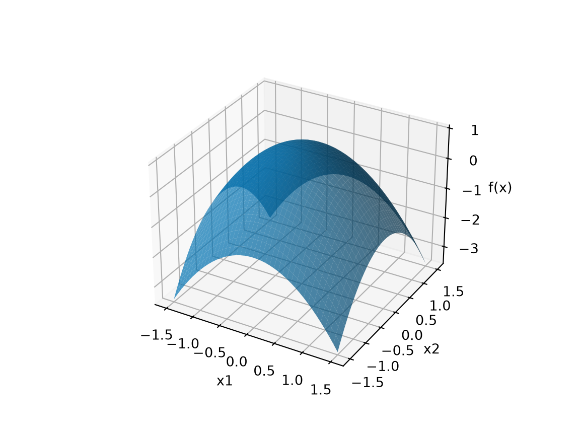
Figure 12: The graph of the strictly concave function \(f(\mathord{\smash[b]{\underset{\raise.3ex\hbox{$\scriptstyle\sim$}}{x}}\vphantom{x}}) = 1 - x_1^2 - x_2^2\) of Example 16 is a dome with its highest point at \(\mathord{\smash[b]{\underset{\raise.3ex\hbox{$\scriptstyle\sim$}}{0}}\vphantom{0}}\).

• R
• Python

Corollary 2 (Stationary points of a convex function are global minimizers) If \(f\) is as in Theorem 5 and convex, then every stationary point \(\mathord{\smash[b]{\underset{\raise.3ex\hbox{$\scriptstyle\sim$}}{x}}\vphantom{x}}^*\) of \(f\) (Definition 4 in Critical Points and Optimality Conditions) is a global minimizer.

Proof. For every \(\mathord{\smash[b]{\underset{\raise.3ex\hbox{$\scriptstyle\sim$}}{x}}\vphantom{x}}\),

\[ \begin{aligned} f(\mathord{\smash[b]{\underset{\raise.3ex\hbox{$\scriptstyle\sim$}}{x}}\vphantom{x}}) &\ge f(\mathord{\smash[b]{\underset{\raise.3ex\hbox{$\scriptstyle\sim$}}{x}}\vphantom{x}}^*) + {\mathopen{}\left(\frac{\partial}{\partial \mathord{\smash[b]{\underset{\raise.3ex\hbox{$\scriptstyle\sim$}}{x}}\vphantom{x}}} f(\mathord{\smash[b]{\underset{\raise.3ex\hbox{$\scriptstyle\sim$}}{x}}\vphantom{x}}^*)\right)\mathclose{}}^{\top} (\mathord{\smash[b]{\underset{\raise.3ex\hbox{$\scriptstyle\sim$}}{x}}\vphantom{x}}- \mathord{\smash[b]{\underset{\raise.3ex\hbox{$\scriptstyle\sim$}}{x}}\vphantom{x}}^*) && \text{(}\href{#eq-supporting-hyperplane}{\text{Equation~1}}\text{ with } \mathord{\smash[b]{\underset{\raise.3ex\hbox{$\scriptstyle\sim$}}{y}}\vphantom{y}}= \mathord{\smash[b]{\underset{\raise.3ex\hbox{$\scriptstyle\sim$}}{x}}\vphantom{x}}^* \text{)} \\ &= f(\mathord{\smash[b]{\underset{\raise.3ex\hbox{$\scriptstyle\sim$}}{x}}\vphantom{x}}^*) + {\mathord{\smash[b]{\underset{\raise.3ex\hbox{$\scriptstyle\sim$}}{0}}\vphantom{0}}}^{\top} (\mathord{\smash[b]{\underset{\raise.3ex\hbox{$\scriptstyle\sim$}}{x}}\vphantom{x}}- \mathord{\smash[b]{\underset{\raise.3ex\hbox{$\scriptstyle\sim$}}{x}}\vphantom{x}}^*) && \text{(} \mathord{\smash[b]{\underset{\raise.3ex\hbox{$\scriptstyle\sim$}}{x}}\vphantom{x}}^* \text{ is stationary)} \\ &= f(\mathord{\smash[b]{\underset{\raise.3ex\hbox{$\scriptstyle\sim$}}{x}}\vphantom{x}}^*). && \text{(} \mathord{\smash[b]{\underset{\raise.3ex\hbox{$\scriptstyle\sim$}}{0}}\vphantom{0}} \cdot \mathord{\smash[b]{\underset{\raise.3ex\hbox{$\scriptstyle\sim$}}{v}}\vphantom{v}} = 0 \text{)} \end{aligned} \]

Example 17 (A convex function, and a non-convex one)  

• \(f(\mathord{\smash[b]{\underset{\raise.3ex\hbox{$\scriptstyle\sim$}}{x}}\vphantom{x}}) = x_1^2 + x_2^2 - 2 x_1\) is convex by Theorem 6, since its Hessian is \(2 \mathbf{I}_2\) (Example 16 in Critical Points and Optimality Conditions), so its stationary point \({(1, 0)}^{\top}\) (Example 8 in Critical Points and Optimality Conditions) is a global minimizer, as completing the square showed in Example 9 in Critical Points and Optimality Conditions.
• Without convexity, a stationary point need not be a minimizer at all: \(x_1^2 - x_2^2\) has the stationary point \(\mathord{\smash[b]{\underset{\raise.3ex\hbox{$\scriptstyle\sim$}}{0}}\vphantom{0}}\), which is not a minimizer (Example 9 in Critical Points and Optimality Conditions).
• The corollary says nothing about whether a minimizer exists: \(e^{2x_1 + x_2} - x_1\) is convex (Example 14) but has no stationary point, and so no local minimizer (Example 9 in Critical Points and Optimality Conditions).

Definition 11 (Convex optimization problem, convex problem) A minimization problem whose objective function is convex and whose feasible set is a convex set is a convex optimization problem (or convex problem) [6].

Example 18 (Minimizing over a line, and over a circle) Let \(f(\mathord{\smash[b]{\underset{\raise.3ex\hbox{$\scriptstyle\sim$}}{x}}\vphantom{x}}) = x_1^2 + x_2^2\). Its Hessian is \(2 \mathbf{I}_2\) at every \(\mathord{\smash[b]{\underset{\raise.3ex\hbox{$\scriptstyle\sim$}}{x}}\vphantom{x}}\), which is positive semidefinite, so \(f\) is convex by part 1 of Theorem 6.

• Minimizing \(f\) subject to \(3 x_1 + 4 x_2 = 5\), as in the example of a minimization problem, is a convex problem. Its feasible set \(L = \mathopen{}\left\{\mathord{\smash[b]{\underset{\raise.3ex\hbox{$\scriptstyle\sim$}}{x}}\vphantom{x}}\in \mathbb{R}^2 : 3 x_1 + 4 x_2 = 5\right\}\mathclose{}\) is a convex set: for \(\mathord{\smash[b]{\underset{\raise.3ex\hbox{$\scriptstyle\sim$}}{x}}\vphantom{x}}, \mathord{\smash[b]{\underset{\raise.3ex\hbox{$\scriptstyle\sim$}}{y}}\vphantom{y}}\in L\) and \(t \in [0, 1]\),

  \[ \begin{aligned} 3 \mathopen{}\left(t x_1 + (1 - t) y_1\right)\mathclose{} + 4 \mathopen{}\left(t x_2 + (1 - t) y_2\right)\mathclose{} &= t \mathopen{}\left(3 x_1 + 4 x_2\right)\mathclose{} + (1 - t) \mathopen{}\left(3 y_1 + 4 y_2\right)\mathclose{} && \text{(distribute and regroup)} \\ &= 5 t + 5 (1 - t) && \text{(} \mathord{\smash[b]{\underset{\raise.3ex\hbox{$\scriptstyle\sim$}}{x}}\vphantom{x}}, \mathord{\smash[b]{\underset{\raise.3ex\hbox{$\scriptstyle\sim$}}{y}}\vphantom{y}}\in L \text{)} \\ &= 5, && \text{(arithmetic)} \end{aligned} \]

  so \(t \mathord{\smash[b]{\underset{\raise.3ex\hbox{$\scriptstyle\sim$}}{x}}\vphantom{x}}+ (1 - t) \mathord{\smash[b]{\underset{\raise.3ex\hbox{$\scriptstyle\sim$}}{y}}\vphantom{y}}\in L\).

• Minimizing the same \(f\) subject to \(x_1^2 + x_2^2 = 1\) is not a convex problem, because its feasible set, the unit circle \(C\), is not a convex set: \({(1, 0)}^{\top}\) and \({(-1, 0)}^{\top}\) are in \(C\), but with \(t = \tfrac{1}{2}\) the point \(\mathord{\smash[b]{\underset{\raise.3ex\hbox{$\scriptstyle\sim$}}{0}}\vphantom{0}}\) is not, since \(0^2 + 0^2 = 0 \ne 1\).

Figure 13 shows both feasible sets.

cop_x1_fc <- seq(-1.5, 2.5, length.out = 2)
cop_x2_fc <- (5 - 3 * cop_x1_fc) / 4
cop_line_fc <- tibble::tibble(x1 = cop_x1_fc, x2 = cop_x2_fc)
cop_angle_fc <- seq(0, 2 * pi, length.out = 201)
cop_cos_fc <- cos(cop_angle_fc)
cop_sin_fc <- sin(cop_angle_fc)
cop_circle_fc <- tibble::tibble(x1 = cop_cos_fc, x2 = cop_sin_fc)
cop_line_pts_x1_fc <- c(-1, 1)
cop_line_pts_x2_fc <- c(2, 0.5)
cop_line_pts_fc <- tibble::tibble(
  x1 = cop_line_pts_x1_fc,
  x2 = cop_line_pts_x2_fc
)
cop_circle_pts_x1_fc <- c(-1, 1)
cop_circle_pts_x2_fc <- c(0, 0)
cop_circle_pts_fc <- tibble::tibble(
  x1 = cop_circle_pts_x1_fc,
  x2 = cop_circle_pts_x2_fc
)
cop_origin_fc <- tibble::tibble(x1 = 0, x2 = 0)
cop_aes_fc <- ggplot2::aes(x = x1, y = x2)
ggplot2::ggplot() +
  ggplot2::geom_line(
    data = cop_line_fc, mapping = cop_aes_fc, colour = "#0072B2"
  ) +
  ggplot2::geom_point(
    data = cop_line_pts_fc, mapping = cop_aes_fc,
    colour = "#0072B2", size = 3
  ) +
  ggplot2::geom_path(
    data = cop_circle_fc, mapping = cop_aes_fc, colour = "#D55E00"
  ) +
  ggplot2::geom_line(
    data = cop_circle_pts_fc, mapping = cop_aes_fc,
    colour = "#D55E00", linetype = "dashed"
  ) +
  ggplot2::geom_point(
    data = cop_circle_pts_fc, mapping = cop_aes_fc,
    colour = "#D55E00", size = 3
  ) +
  ggplot2::geom_point(
    data = cop_origin_fc, mapping = cop_aes_fc,
    colour = "#D55E00", shape = 21, fill = "white", size = 3
  ) +
  ggplot2::coord_fixed() +
  ggplot2::labs(x = "x1", y = "x2")

import matplotlib.pyplot as plt
import numpy as np

cop_x1_fc = np.array([-1.5, 2.5])
cop_angle_fc = np.linspace(0, 2 * np.pi, 201)
fig, ax = plt.subplots(figsize=(4.5, 4.5), layout="constrained")
ax.plot(cop_x1_fc, (5 - 3 * cop_x1_fc) / 4, color="#0072B2");
ax.plot([-1, 1], [2, 0.5], "o", color="#0072B2", markersize=8);
ax.plot(np.cos(cop_angle_fc), np.sin(cop_angle_fc), color="#D55E00");
ax.plot([-1, 1], [0, 0], "o--", color="#D55E00", markersize=8);
ax.plot(0, 0, "o", color="#D55E00", markerfacecolor="white", markersize=8);
ax.set_aspect("equal");
ax.set_xlabel("x1");
ax.set_ylabel("x2");
plt.show();

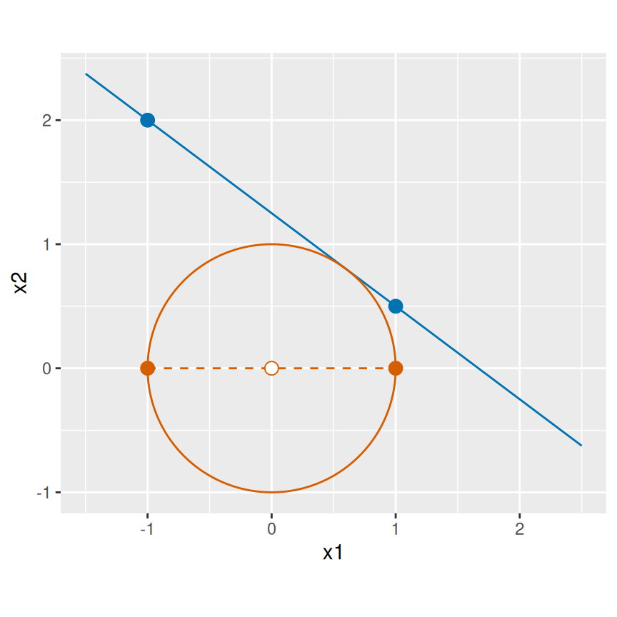
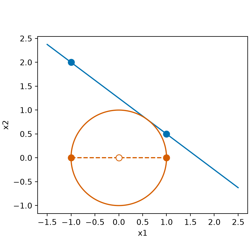
Figure 13: The two feasible sets of Example 18. The segment between two points of the line stays on the line, so minimizing over the line is a convex problem. The segment between two points of the circle leaves it, through \(\mathord{\smash[b]{\underset{\raise.3ex\hbox{$\scriptstyle\sim$}}{0}}\vphantom{0}}\), so minimizing over the circle is not.

• R
• Python

Theorem 9 (The exponential function lies above its tangent line at zero) For every real \(x\),

\[{\operatorname{exp}\mathopen{}\left\{x\right\}\mathclose{}} \ge 1 + x,\]

with equality exactly when \(x = 0\).

Proof. Let \(g(x) = {\operatorname{exp}\mathopen{}\left\{x\right\}\mathclose{}} - 1 - x\). The exponential function has second derivative \({\operatorname{exp}\mathopen{}\left\{x\right\}\mathclose{}} > 0\) at every \(x\), so it is convex by Theorem 6. The function \(g\) differs from it by a linear function, so \(g\) is convex too. The derivative of \(g\) is \(\frac{d g(x)}{d x} = {\operatorname{exp}\mathopen{}\left\{x\right\}\mathclose{}} - 1\), which is \(0\) at \(x = 0\). By Corollary 2, \(0\) is a global minimizer of \(g\), and \(g(0) = 0\), so \(g(x) \ge 0\) for every \(x\).

Suppose \(g(x) = 0\) for some \(x\). Then \(x\) is also a global minimizer of \(g\), and so a local minimizer. Fermat’s theorem gives \(\frac{d g(x)}{d x} = {\operatorname{exp}\mathopen{}\left\{x\right\}\mathclose{}} - 1 = 0\). Then \({\operatorname{exp}\mathopen{}\left\{x\right\}\mathclose{}} = 1 = {\operatorname{exp}\mathopen{}\left\{0\right\}\mathclose{}}\), which gives \(x = 0\) because the exponential function is injective.

Corollary 3 (The natural logarithm lies below its tangent line at one) For every \(t > 0\),

\[{\operatorname{log}\mathopen{}\left\{t\right\}\mathclose{}} \le t - 1,\]

with equality exactly when \(t = 1\).

Proof. Put \(x = {\operatorname{log}\mathopen{}\left\{t\right\}\mathclose{}}\), so that \({\operatorname{exp}\mathopen{}\left\{x\right\}\mathclose{}} = t\) by the inverse relation of the logarithm and the exponential. By Theorem 9, \(t = {\operatorname{exp}\mathopen{}\left\{x\right\}\mathclose{}} \ge 1 + x = 1 + {\operatorname{log}\mathopen{}\left\{t\right\}\mathclose{}}\), which is \({\operatorname{log}\mathopen{}\left\{t\right\}\mathclose{}} \le t - 1\). Equality holds exactly when \(x = 0\), that is, when \({\operatorname{log}\mathopen{}\left\{t\right\}\mathclose{}} = 0\), that is, when \(t = 1\).

Example 19 (Two values of the bounds)  

At \(x = 1\), \({\operatorname{exp}\mathopen{}\left\{1\right\}\mathclose{}} = \text{e}\approx 2.718\), which is at least \(1 + 1 = 2\). At \(t = 2\), \({\operatorname{log}\mathopen{}\left\{2\right\}\mathclose{}} \approx 0.693\), which is at most \(2 - 1 = 1\). Neither is an equality, because \(x \ne 0\) and \(t \ne 1\).

[1]

H. Zhou, “Optimization and multivariate calculus.” Lecture notes for Biostat 216, Mathematical Methods for Biostatistics, University of California, Los Angeles, 2024. Accessed: Oct. 05, 2026. [Online]. Available: https://ucla-biostat-216.github.io/2024fall/slides/13-optim/13-optim.html

[2]

Wikipedia contributors, “Convex set — Wikipedia, the free encyclopedia.” 2026. Available: https://en.wikipedia.org/wiki/Convex_set

[3]

Wikipedia contributors, “Convex hull — Wikipedia, the free encyclopedia.” 2026. Available: https://en.wikipedia.org/wiki/Convex_hull

[4]

Wikipedia contributors, “Epigraph (mathematics) — Wikipedia, the free encyclopedia.” 2026. Available: https://en.wikipedia.org/wiki/Epigraph_(mathematics)

[5]

Wikipedia contributors, “Tangent space — Wikipedia, the free encyclopedia.” 2026. Available: https://en.wikipedia.org/wiki/Tangent_space

[6]

Wikipedia contributors, “Convex optimization — Wikipedia, the free encyclopedia.” 2026. Available: https://en.wikipedia.org/wiki/Convex_optimization