Double Integrals and Fubini’s Theorem

Last modified: 2026-10-27 20:53:54 (PDT)

1 Double Integrals

The Fubini–Tonelli theorem states conditions under which the order of integration in a double integral can be exchanged [1]. We state them in two settings: the Riemann version (Theorem 1) is what applied courses usually use for double integrals of continuous functions on simple regions; the \(\sigma\)-finite measure-theoretic versions (Theorem 4 and Theorem 5) are included to make the joint-distribution form corollary in Probability for Data Science follow from a stated theorem rather than from an aside.

Definition 1 (Double integral) Let \(f\) be a bounded function on a closed, bounded plane region \(R \subseteq \mathbb{R}^2\) [2]. Cover \(R\) with a grid of rectangles, keep the \(n\) rectangles that lie entirely inside \(R\), with areas \(\Delta A_1, \ldots, \Delta A_n\), and choose a point \((x_i, y_i)\) in the \(i\)-th rectangle. The double integral of \(f\) over \(R\) is

\[\iint_R f(x, y)\,dA \stackrel{\text{def}}{=}\lim_{\mathopen{}\left\lVert\Delta\right\rVert\mathclose{} \to 0} \sum_{i=1}^nf(x_i, y_i)\,\Delta A_i,\]

where \(\mathopen{}\left\lVert\Delta\right\rVert\mathclose{}\) is the length of the longest diagonal among the \(n\) rectangles, when that limit exists and has the same value for every choice of grids and of the points \((x_i, y_i)\). The symbol \(dA\) stands for an element of area.

[3, Sec. 14.2]

Example 1 (The double integral of \(1\) is an area) Let \(f(x, y) = 1\) on the rectangle \(R = [0, 2] \times [0, 3]\). Every sum in Definition 1 adds up the areas of rectangles inside \(R\), and those sums approach the area of \(R\) as the grid gets finer, so

\[ \begin{aligned} \iint_R 1\,dA &= 2 \cdot 3 \\ &= 6. \end{aligned} \]

Definition 2 (Iterated integral) An iterated integral is an integral of an integral [4]:

\[ \int_a^b \int_{g_1(x)}^{g_2(x)} f(x, y)\,dy\,dx \stackrel{\text{def}}{=}\int_a^b \mathopen{}\left(\int_{g_1(x)}^{g_2(x)} f(x, y)\,dy\right)\mathclose{}\,dx \]

That is, integrate over the inner variable (\(y\)) first, holding the outer variable (\(x\)) fixed, and then integrate the result over the outer variable. The inner limits \(g_1(x)\) and \(g_2(x)\) may depend on the outer variable, or be constants \(c\) and \(d\), as in \(\int_a^b \int_c^d f(x, y)\,dy\,dx\). Iterated integrals in the other order, \(\int \int \cdots \,dx\,dy\), are defined the same way with the roles of \(x\) and \(y\) swapped.

Example 2 (An iterated integral) Integrating over \(y\) first, then \(x\):

\[ \begin{aligned} \int_0^1 \int_0^2 x y\,dy\,dx &= \int_0^1 \mathopen{}\left(\int_0^2 x y\,dy\right)\mathclose{}\,dx && \text{(definition of the iterated integral)} \\ &= \int_0^1 x \mathopen{}\left(\int_0^2 y\,dy\right)\mathclose{}\,dx && \text{(} x \text{ is constant in } y \text{)} \\ &= \int_0^1 x \mathopen{}\left[\frac{y^2}{2}\right]\mathclose{}_{y=0}^{y=2}\,dx && \text{(antiderivative of } y \text{)} \\ &= \int_0^1 2x\,dx && \text{(evaluate at the limits)} \\ &= \mathopen{}\left[x^2\right]\mathclose{}_{x=0}^{x=1} && \text{(antiderivative of } 2x \text{)} \\ &= 1 && \text{(evaluate at the limits)} \end{aligned} \]

Theorem 1 (Fubini’s theorem (Riemann version)) Let \(f\) be continuous on a plane region \(R \subseteq \mathbb{R}^2\) [5].

Vertically simple region. If \(R\) is defined by \(a \le x \le b\) and \(g_1(x) \le y \le g_2(x)\), where \(g_1\) and \(g_2\) are continuous on \([a, b]\), then

\[ \begin{aligned} \iint_R f(x, y)\,dA &= \int_a^b \int_{g_1(x)}^{g_2(x)} f(x, y)\,dy\,dx. \end{aligned} \]
Horizontally simple region. If \(R\) is defined by \(c \le y \le d\) and \(h_1(y) \le x \le h_2(y)\), where \(h_1\) and \(h_2\) are continuous on \([c, d]\), then

\[ \begin{aligned} \iint_R f(x, y)\,dA &= \int_c^d \int_{h_1(y)}^{h_2(y)} f(x, y)\,dx\,dy. \end{aligned} \]

When \(R\) can be described both ways, the two iterated integrals are equal — so the order of integration can be exchanged.

[3], Theorem 14.2, p. 982

Example 3 (Changing the order of integration for a non-rectangular region) Adapted from [3, Sec. 14.2], Example 4, pp. 984–985.

Let \(X\) and \(Y\) be independent \(\operatorname{Uniform}(0, 1)\) random variables, with joint density \(f(x, y) = 1\) on the unit square \([0, 1]^2\). Define the function \(g(x, y) = \text{e}^{-x^2}\,{\mathbb{1}\mathopen{}\left(y \le x\right)\mathclose{}}\), where \(e\) is Euler’s number, and compute its expectation \({\mathbb{E}\mathopen{}\left[g(X, Y)\right]\mathclose{}}\).

Because the joint density equals \(1\) on \([0, 1]^2\), this expectation is the double integral of \(g\) over the unit square:

\[{\mathbb{E}\mathopen{}\left[g(X, Y)\right]\mathclose{}} = \iint_{[0, 1]^2} g(x, y)\,dA.\]

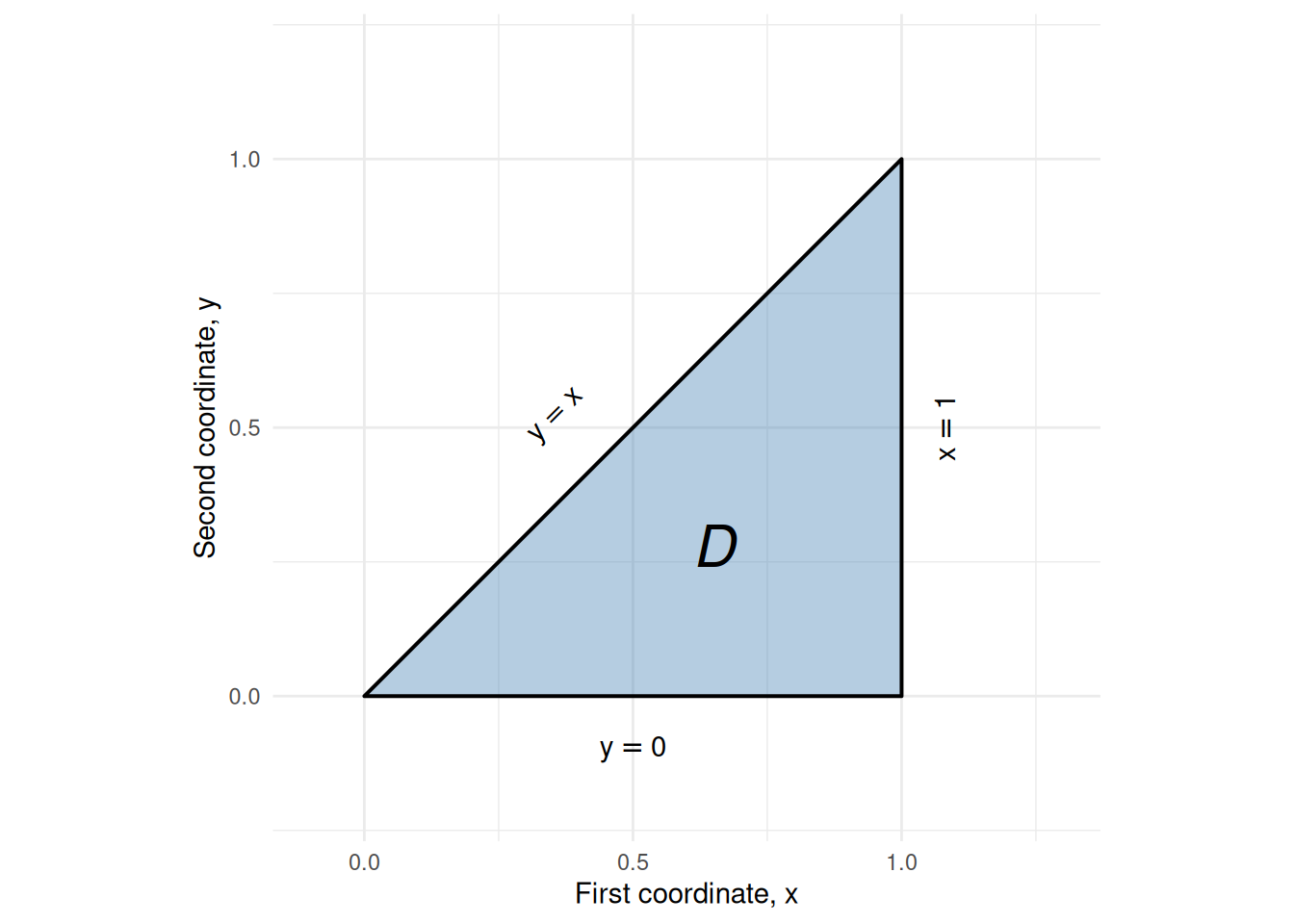
The indicator factor \({\mathbb{1}\mathopen{}\left(y \le x\right)\mathclose{}}\) equals \(1\) on the triangular region where \(y \le x\) and \(0\) elsewhere, so only that region, namely \(D = \{(x, y) : x \in [0, 1],\; y \in [0, x]\}\) (Figure 1), contributes, and there \(g(x, y) = \text{e}^{-x^2}\):

\[{\mathbb{E}\mathopen{}\left[g(X, Y)\right]\mathclose{}} = \iint_D \text{e}^{-x^2}\,dA.\]

[R code]

region <- tibble::tibble(x = c(0, 1, 1), y = c(0, 0, 1))
ggplot2::ggplot(region, ggplot2::aes(x = x, y = y)) +
  ggplot2::geom_polygon(
    fill = "steelblue", alpha = 0.4, color = "black", linewidth = 0.7
  ) +
  ggplot2::annotate(
    "text", x = 0.65, y = 0.28, label = "D", size = 8, fontface = "italic"
  ) +
  ggplot2::annotate(
    "text", x = 0.36, y = 0.52, label = "y == x",
    parse = TRUE, angle = 45
  ) +
  ggplot2::annotate(
    "text", x = 1.08, y = 0.5, label = "x == 1",
    parse = TRUE, angle = 90, hjust = 0.5
  ) +
  ggplot2::annotate(
    "text", x = 0.5, y = -0.1, label = "y == 0", parse = TRUE
  ) +
  ggplot2::scale_x_continuous(breaks = c(0, 0.5, 1), limits = c(-0.1, 1.3)) +
  ggplot2::scale_y_continuous(breaks = c(0, 0.5, 1), limits = c(-0.2, 1.2)) +
  ggplot2::coord_equal() +
  ggplot2::labs(x = "First coordinate, x", y = "Second coordinate, y") +
  ggplot2::theme_minimal()

Figure 1: Triangular integration region \(D = \{(x, y) : x \in [0, 1],\; y \in [0, x]\}\), bounded below by \(y = 0\), above-left by \(y = x\), and on the right by \(x = 1\).

Order \(dx\,dy\) is intractable. Re-describing \(D\) as \(D = \{(x, y) : y \in [0, 1],\; x \in [y, 1]\}\), the inner integral is

\[\int_y^1 \text{e}^{-x^2}\,dx,\]

which cannot be computed with FTC Part 2: no antiderivative of \(\text{e}^{-x^2}\) can be written as a finite formula built from powers, exponentials, logarithms, and trigonometric functions (an elementary antiderivative).

Order \(dy\,dx\) works. Applying Theorem 1 Part 1 (\(\text{e}^{-x^2}\) is continuous and \(D\) is the vertically simple region \(x \in [0, 1]\), \(y \in [0, x]\)):

\[ \begin{aligned} \iint_D \text{e}^{-x^2}\,dA &= \int_0^1\!\int_0^x \text{e}^{-x^2}\,dy\,dx && \text{(Fubini, vertically simple region)} \\&= \int_0^1 \text{e}^{-x^2}\mathopen{}\left(\int_0^x dy\right)\mathclose{}\,dx && \text{(} \text{e}^{-x^2} \text{ is constant in } y \text{)} \\&= \int_0^1 x\,\text{e}^{-x^2}\,dx && \text{(} \textstyle\int_0^x dy = x \text{)} \end{aligned} \]

To antidifferentiate \(x\,\text{e}^{-x^2}\), let \(u = x^2\) be the inner function. By the chain rule (Theorem 10 in Derivatives and Taylor Series), with \(\frac{d u}{d x} = 2x\),

\[ \begin{aligned} \frac{d }{d x}\mathopen{}\left(-\frac{1}{2}\,\text{e}^{-u}\right)\mathclose{} &= -\frac{1}{2}\,\text{e}^{-u} \cdot(-1) \cdot\frac{d u}{d x} && \text{(chain rule)} \\&= -\frac{1}{2}\,\text{e}^{-x^2} \cdot(-1) \cdot 2x && \text{(substitute } u = x^2 \text{ and } du/dx = 2x \text{)} \\&= x\,\text{e}^{-x^2} && \text{(multiply)} \end{aligned} \]

so \(-\frac{1}{2}\,\text{e}^{-x^2}\) is an antiderivative of \(x\,\text{e}^{-x^2}\), and

\[ \begin{aligned} \int_0^1 x\,\text{e}^{-x^2}\,dx &= \mathopen{}\left[-\frac{1}{2}\,\text{e}^{-x^2}\right]\mathclose{}_0^1 && \text{(FTC Part 2)} \\&= -\frac{1}{2}\mathopen{}\left(\text{e}^{-1} - \text{e}^{0}\right)\mathclose{} && \text{(evaluate at the limits)} \\&= -\frac{1}{2}\mathopen{}\left(\text{e}^{-1} - 1\right)\mathclose{} && \text{(} \text{e}^{0} = 1 \text{)} \\&= \frac{1 - \text{e}^{-1}}{2} && \text{(distribute } -\tfrac{1}{2} \text{)} \\&= \frac{e - 1}{2e} && \text{(multiply numerator and denominator by } e \text{)} \\&\approx 0.316 \end{aligned} \]

The solid whose volume equals this integral is shown in Figure 2.

[R code]

n_grid <- 51
x_seq <- seq(0, 1, length.out = n_grid)
y_seq <- seq(0, 1, length.out = n_grid)

z_mat <- outer(x_seq, y_seq, function(x, y) {
  z <- exp(-x^2)
  z[y > x] <- NA
  z
})

plotly::plot_ly(x = ~x_seq, y = ~y_seq, z = ~t(z_mat)) |>
  plotly::add_surface(showscale = FALSE) |>
  plotly::layout(scene = list(
    xaxis = list(title = "First coordinate, x"),
    yaxis = list(title = "Second coordinate, y"),
    zaxis = list(title = "z = exp(-x^2)"),
    camera = list(eye = list(x = 1.6, y = -1.6, z = 0.8))
  ))

Figure 2: Surface \(z = e^{-x^2}\) over the region \(D = \{(x, y) : x \in [0, 1],\; y \in [0, x]\}\). The surface depends only on \(x\) (constant in \(y\)), so for each \(x\) the inner integral over \(y \in [0, x]\) contributes \(x \cdot e^{-x^2}\).

Exercise 1 (Double integral over a triangular region) Adapted from Miller [6], Question 1.1.50.

Evaluate the integral:

\[\int_0^1 \int_0^x xy\,dy\,dx\]

and confirm the result by reversing the order of integration.

Solution 1. 1. Given order (\(y\) then \(x\)):

\[ \begin{aligned} \int_0^x xy\,dy &= x\mathopen{}\left[\frac{y^2}{2}\right]\mathclose{}_0^x \\ &= \frac{x^3}{2} \end{aligned} \]

\[ \begin{aligned} \int_0^1 \frac{x^3}{2}\,dx &= \mathopen{}\left[\frac{x^4}{8}\right]\mathclose{}_0^1 \\ &= \frac{1}{8} \end{aligned} \]

2. Reversed order (\(x\) then \(y\)): The triangular region \(T = \{(x, y) : 0 \le x \le 1, 0 \le y \le x\}\) is equivalently described by \(T = \{(x, y) : 0 \le y \le 1, y \le x \le 1\}\):

\[ \begin{aligned} \int_0^1 \int_y^1 xy\,dx\,dy &= \int_0^1 y\mathopen{}\left[\frac{x^2}{2}\right]\mathclose{}_{x=y}^1\,dy \\ &= \int_0^1 \frac{y(1 - y^2)}{2}\,dy \end{aligned} \]

\[ \begin{aligned} \int_0^1 \mathopen{}\left(\frac{y}{2} - \frac{y^3}{2}\right)\mathclose{}\,dy &= \mathopen{}\left[\frac{y^2}{4} - \frac{y^4}{8}\right]\mathclose{}_0^1 \\ &= \frac{1}{4} - \frac{1}{8} \\ &= \frac{1}{8} \end{aligned} \]

Both orders yield \(1/8\).

Exercise 2 (Switching order of integration on a non-rectangular region) Adapted from Miller [6], Question 1.1.51.

Express the integral:

\[\int_0^1 \int_0^x y e^{-xy}\,dy\,dx\]

by reversing the order of integration.

Solution 2. In the given order, the inner integral \(\int_0^x y e^{-xy}\,dy\) requires integration by parts with respect to \(y\).

Switching the order over the triangular domain \(\{(x, y) : 0 \le y \le 1, y \le x \le 1\}\):

\[\int_0^1 \int_y^1 y e^{-xy}\,dx\,dy\]

Now the inner integral has the factor \(y\) in place for direct integration with respect to \(x\):

\[ \begin{aligned} \int_y^1 y e^{-xy}\,dx &= \mathopen{}\left[-e^{-xy}\right]\mathclose{}_{x=y}^1 \\ &= e^{-y^2} - e^{-y} \end{aligned} \]

The double integral becomes:

\[ \begin{aligned} \int_0^1 (e^{-y^2} - e^{-y})\,dy &= \int_0^1 e^{-y^2}\,dy - \mathopen{}\left[-e^{-y}\right]\mathclose{}_0^1 \\ &= \int_0^1 e^{-y^2}\,dy - (1 - e^{-1}) \end{aligned} \]

The term \(\int_0^1 e^{-y^2}\,dy\) has no elementary antiderivative; it can be written using the error function \(\operatorname{erf}(z) = \frac{2}{\sqrt{\pi}}\int_0^z e^{-t^2}\,dt\) as \(\frac{\sqrt{\pi}}{2}\operatorname{erf}(1) \approx 0.7468\). The overall value is:

\[\frac{\sqrt{\pi}}{2}\operatorname{erf}(1) + e^{-1} - 1 \approx 0.1147\]

Example 4 (When conditions fail: a counterexample) The conditions in Theorem 1 are not merely technical — when they fail, iterated integrals can exist yet disagree.

Let \[f(x, y) = \frac{x^2 - y^2}{(x^2 + y^2)^2}\] on the unit square \(R = [0, 1] \times [0, 1]\). Strictly, \(f\) is defined on \(R \setminus \{(0, 0)\}\): the denominator vanishes at the origin, so \(f\) is undefined there (we return to this point in the condition check).

Integrating \(y\) first, then \(x\):

Holding \(x\) fixed and differentiating in \(y\) (by the quotient rule, Theorem 9 in Derivatives and Taylor Series),

\[ \begin{aligned} \frac{d }{d y}\frac{y}{x^2 + y^2} &= \frac{(x^2 + y^2) - y \cdot 2y}{(x^2 + y^2)^2} \\ &= \frac{x^2 - y^2}{(x^2 + y^2)^2}. \end{aligned} \]

(A derivative in one variable with the others held fixed is a partial derivative, defined on the vector calculus page.) The arctangent \(\arctan\) is the inverse of the tangent function from trigonometry; all this example needs is that \(\frac{d }{d x}\arctan(x) = \frac{1}{1 + x^2}\), \(\arctan(0) = 0\), and \(\arctan(1) = \frac{\pi}{4}\).

\[ \begin{aligned} \int_0^1\!\int_0^1 f(x, y)\,dy\,dx &= \int_0^1 \mathopen{}\left[\frac{y}{x^2 + y^2}\right]\mathclose{}_{y=0}^{y=1}\,dx \\&= \int_0^1 \frac{1}{x^2 + 1}\,dx \\&= \mathopen{}\left[\arctan(x)\right]\mathclose{}_0^1 \\&= \frac{\pi}{4} \end{aligned} \]

Integrating \(x\) first, then \(y\):

Holding \(y\) fixed and differentiating in \(x\),

\[ \begin{aligned} \frac{d }{d x}\mathopen{}\left(-\frac{x}{x^2 + y^2}\right)\mathclose{} &= -\frac{(x^2 + y^2) - x \cdot 2x}{(x^2 + y^2)^2} \\ &= \frac{x^2 - y^2}{(x^2 + y^2)^2}: \end{aligned} \]

\[ \begin{aligned} \int_0^1\!\int_0^1 f(x, y)\,dx\,dy &= \int_0^1 \mathopen{}\left[-\frac{x}{x^2 + y^2}\right]\mathclose{}_{x=0}^{x=1}\,dy \\&= \int_0^1 \mathopen{}\left(-\frac{1}{1 + y^2}\right)\mathclose{}\,dy \\&= -\mathopen{}\left[\arctan(y)\right]\mathclose{}_0^1 \\&= -\frac{\pi}{4} \end{aligned} \]

Conclusion: \(\dfrac{\pi}{4} \neq -\dfrac{\pi}{4}\), so the two iterated integrals are unequal. Theorem 1 does not apply here.

Why Theorem 1’s condition fails: Theorem 1 requires \(f\) to be continuous on \(R\). The denominator \((x^2 + y^2)^2\) vanishes at the origin \((0, 0) \in R\), so \(f\) is not even defined there — let alone continuous — and the theorem does not apply.

[5]

Figure 3 shows the surface. The failure comes from the origin, where \(f\) is undefined and unbounded.

[R code]

n_grid <- 81
eps <- 0.04
x_seq <- seq(eps, 1, length.out = n_grid)
y_seq <- seq(eps, 1, length.out = n_grid)

z_mat <- outer(x_seq, y_seq, function(x, y) (x^2 - y^2) / (x^2 + y^2)^2)
z_clip <- 50
z_mat[z_mat > z_clip] <- z_clip
z_mat[z_mat < -z_clip] <- -z_clip

plotly::plot_ly(x = ~x_seq, y = ~y_seq, z = ~t(z_mat)) |>
  plotly::add_surface(
    showscale = FALSE,
    colorscale = list(
      list(0, "#3b4cc0"),
      list(0.5, "#dddddd"),
      list(1, "#b40426")
    )
  ) |>
  plotly::layout(scene = list(
    xaxis = list(title = "First coordinate, x"),
    yaxis = list(title = "Second coordinate, y"),
    zaxis = list(title = "f(x, y)", range = c(-z_clip, z_clip)),
    camera = list(eye = list(x = 1.6, y = 1.6, z = 0.6))
  ))

Figure 3: Surface \(f(x, y) = (x^2 - y^2)/(x^2 + y^2)^2\) on \([0, 1]^2\), sampled away from the origin and clipped to \([-50, 50]\) for display. Approaching the origin, the function grows without bound along the \(x\)-axis (red ridge, \(f > 0\) when \(|x| > |y|\)) and falls without bound along the \(y\)-axis (blue ridge, \(f < 0\) when \(|y| > |x|\)). Because \(f\) is undefined at \((0, 0)\), \(f\) is not continuous on \(R\) and Theorem 1 does not apply.

Corollary 1 (Continuous functions on a rectangle (corollary of Theorem 1)) If \(f : [a, b] \times [c, d] \to \mathbb{R}\) is continuous on the closed bounded rectangle \([a, b] \times [c, d]\), then:

\[ \begin{aligned} \int_a^b \mathopen{}\left(\int_c^d f(x, y)\,dy\right)\mathclose{}\,dx &= \int_c^d \mathopen{}\left(\int_a^b f(x, y)\,dx\right)\mathclose{}\,dy\\ &= \iint_{[a,b]\times[c,d]} f(x, y)\,dA. \end{aligned} \]

[3], Theorem 14.2, p. 982

Proof. A closed bounded rectangle \([a, b] \times [c, d]\) is both vertically simple (with \(g_1 \equiv c\), \(g_2 \equiv d\)) and horizontally simple (with \(h_1 \equiv a\), \(h_2 \equiv b\)). Applying both parts of Theorem 1 to \(f\) on this rectangle gives the two iterated forms shown.

Example 5 (Evaluating a double integral on a rectangle) Structure adapted from [3, Sec. 14.2], Example 2, pp. 982–983; the integrand \(x^2 + y^2\) is original, chosen so the integral equals \({\mathbb{E}\mathopen{}\left[g(X, Y)\right]\mathclose{}}\) for \(g(x, y) = x^2 + y^2\).

Let \(X\) and \(Y\) be independent \(\operatorname{Uniform}(0, 1)\) random variables, with joint density \(f(x, y) = 1\) on the unit square \(R = \{(x, y) : x \in [0, 1],\; y \in [0, 1]\}\) (Figure 4). Define the function \(g(x, y) = x^2 + y^2\), and compute its expectation \({\mathbb{E}\mathopen{}\left[g(X, Y)\right]\mathclose{}}\).

Because the joint density equals \(1\) on \(R\), this expectation is the double integral of \(g\) over \(R\):

\[{\mathbb{E}\mathopen{}\left[g(X, Y)\right]\mathclose{}} = \iint_R \mathopen{}\left(x^2 + y^2\right)\mathclose{}\,dA.\]

[R code]

ggplot2::ggplot() +
  ggplot2::annotate(
    "rect", xmin = 0, xmax = 1, ymin = 0, ymax = 1,
    fill = "steelblue", alpha = 0.4, color = "black", linewidth = 0.7
  ) +
  ggplot2::annotate(
    "text", x = 0.5, y = 0.5, label = "R", size = 8, fontface = "italic"
  ) +
  ggplot2::scale_x_continuous(breaks = c(0, 1), limits = c(-0.15, 1.25)) +
  ggplot2::scale_y_continuous(breaks = c(0, 1), limits = c(-0.15, 1.25)) +
  ggplot2::coord_equal() +
  ggplot2::labs(x = "First coordinate, x", y = "Second coordinate, y") +
  ggplot2::theme_minimal()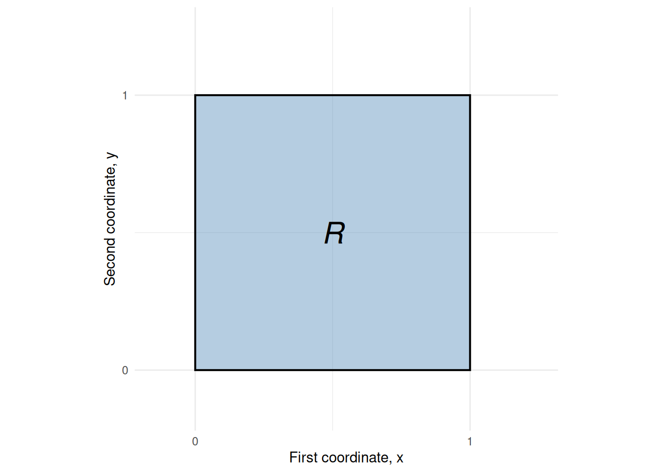

Figure 4: Integration region \(R = [0, 1]^2\), the unit square.

The integrand is continuous on \(R\), so Corollary 1 applies and either order of integration yields the same value.

Integrating \(y\) first, then \(x\):

\[ \begin{aligned} {\mathbb{E}\mathopen{}\left[g(X, Y)\right]\mathclose{}} &= \int_0^1\!\int_0^1 \mathopen{}\left(x^2 + y^2\right)\mathclose{}\,dy\,dx \\&= \int_0^1 \mathopen{}\left[x^2 y + \frac{y^3}{3}\right]\mathclose{}_0^1\,dx \\&= \int_0^1 \mathopen{}\left(x^2 + \frac{1}{3}\right)\mathclose{}\,dx \\&= \mathopen{}\left[\frac{x^3}{3} + \frac{x}{3}\right]\mathclose{}_0^1 \\&= \frac{2}{3} \end{aligned} \]

Integrating \(x\) first, then \(y\) (verifying the order can be swapped):

\[ \begin{aligned} \int_0^1\!\int_0^1 \mathopen{}\left(x^2 + y^2\right)\mathclose{}\,dx\,dy &= \int_0^1 \mathopen{}\left[\frac{x^3}{3} + y^2 x\right]\mathclose{}_0^1\,dy \\&= \int_0^1 \mathopen{}\left(\frac{1}{3} + y^2\right)\mathclose{}\,dy \\&= \mathopen{}\left[\frac{y}{3} + \frac{y^3}{3}\right]\mathclose{}_0^1 \\&= \frac{2}{3} \end{aligned} \]

Both orders give \(\frac{2}{3}\), as Corollary 1 guarantees.

As a cross-check, linearity of expectation gives the same value: since

\[ \begin{aligned} {\mathbb{E}\mathopen{}\left[X^2\right]\mathclose{}} &= \int_0^1 x^2\,dx \\ &= \frac{1}{3} \end{aligned} \]

for \(X \sim \operatorname{Uniform}(0, 1)\) (and likewise for \(Y\)),

\[ \begin{aligned} {\mathbb{E}\mathopen{}\left[g(X, Y)\right]\mathclose{}} &= {\mathbb{E}\mathopen{}\left[X^2 + Y^2\right]\mathclose{}} \\ &= {\mathbb{E}\mathopen{}\left[X^2\right]\mathclose{}} + {\mathbb{E}\mathopen{}\left[Y^2\right]\mathclose{}} \\ &= \frac{1}{3} + \frac{1}{3} \\ &= \frac{2}{3}. \end{aligned} \]

The solid whose volume equals this integral is shown in Figure 5.

[R code]

n_grid <- 41
x_seq <- seq(0, 1, length.out = n_grid)
y_seq <- seq(0, 1, length.out = n_grid)
z_mat <- outer(x_seq, y_seq, function(x, y) x^2 + y^2)

plotly::plot_ly(x = ~x_seq, y = ~y_seq, z = ~t(z_mat)) |>
  plotly::add_surface(showscale = FALSE) |>
  plotly::layout(scene = list(
    xaxis = list(title = "First coordinate, x"),
    yaxis = list(title = "Second coordinate, y"),
    zaxis = list(title = "z", range = c(0, 2))
  ))

Figure 5: Surface \(z = x^2 + y^2\) over the unit square \([0, 1]^2\). The double integral \(\tfrac{2}{3}\) is the volume between this surface and the \(xy\)-plane, and equals \({\mathbb{E}\mathopen{}\left[X^2 + Y^2\right]\mathclose{}}\).

Exercise 3 (Double integral of a polynomial over a rectangle) Adapted from Miller [6], Question 1.1.47.

Evaluate the double integral:

\[\int_0^2 \int_0^3 5(x^2 y + xy^2 + 2)\,dy\,dx\]

Solution 3. Integrate with respect to \(y\) first:

\[\begin{aligned} \int_0^3 (x^2 y + xy^2 + 2)\,dy &= \mathopen{}\left[\frac{x^2 y^2}{2} + \frac{x y^3}{3} + 2y\right]\mathclose{}_{y=0}^3 \\ &= \frac{9}{2}x^2 + 9x + 6 \end{aligned}\]

Now integrate with respect to \(x\):

\[\begin{aligned} 5\int_0^2 \mathopen{}\left(\frac{9}{2}x^2 + 9x + 6\right)\mathclose{}\,dx &= 5\mathopen{}\left[\frac{3}{2}x^3 + \frac{9}{2}x^2 + 6x\right]\mathclose{}_0^2 \\ &= 5\mathopen{}\left[\frac{3}{2}(8) + \frac{9}{2}(4) + 6(2)\right]\mathclose{} \\ &= 5\mathopen{}\left[12 + 18 + 12\right]\mathclose{} \\ &= 5(42) \\ &= 210 \end{aligned}\]

(Note: The source text carried an arithmetic slip in the inner coefficient resulting in \(190\); the exact value is \(210\).)

Exercise 4 (Choosing the order of integration) Adapted from Miller [6], Question 1.1.48.

Evaluate the double integral:

\[\int_0^6 \int_0^5 x e^{-xy}\,dy\,dx\]

Solution 4. Integrating with respect to \(x\) first requires integration by parts. Integrating with respect to \(y\) first is much simpler because the factor of \(x\) is already present:

\[ \begin{aligned} \int_0^5 x e^{-xy}\,dy &= \mathopen{}\left[-e^{-xy}\right]\mathclose{}_{y=0}^5 \\ &= 1 - e^{-5x} \end{aligned} \]

Now integrate with respect to \(x\):

\[\begin{aligned} \int_0^6 (1 - e^{-5x})\,dx &= \mathopen{}\left[x + \frac{1}{5}e^{-5x}\right]\mathclose{}_0^6 \\ &= \mathopen{}\left(6 + \frac{1}{5}e^{-30}\right)\mathclose{} - \mathopen{}\left(0 + \frac{1}{5}\right)\mathclose{} \\ &= \frac{29}{5} + \frac{e^{-30}}{5} \end{aligned}\]

Exercise 5 (Product of single integrals for separable functions) Adapted from Miller [6], Question 1.1.49.

Let \(m, n > 0\). Evaluate:

\[\int_0^1 \int_0^1 x^m y^n\,dy\,dx\]

Solution 5. Because the region of integration is a rectangle \([0, 1] \times [0, 1]\) and the integrand factors as \(g(x)h(y) = x^m \cdot y^n\), the double integral splits into the product of two single-variable integrals:

\[\int_0^1 \int_0^1 x^m y^n\,dy\,dx = \mathopen{}\left(\int_0^1 x^m\,dx\right)\mathclose{}\mathopen{}\left(\int_0^1 y^n\,dy\right)\mathclose{}\]

Evaluating each factor:

\[\int_0^1 x^m\,dx = \frac{1}{m + 1}, \qquad \int_0^1 y^n\,dy = \frac{1}{n + 1}\]

Therefore:

\[\int_0^1 \int_0^1 x^m y^n\,dy\,dx = \frac{1}{(m + 1)(n + 1)}\]

Remark: When joint random variables \(X\) and \(Y\) are independent, their joint density factors as \(f_{X, Y}(x, y) = f_X(x)f_Y(y)\), and joint probabilities over product sets factor in exactly this way.

Theorem 2 (Double integral of a product of powers) For \(m, n > 0\),

\[\int_0^1 \int_0^1 x^m y^n\,dy\,dx = \frac{1}{(m + 1)(n + 1)}\]

Proof. This is the solution to Exercise 5, worked in Solution 5.

Exercise 6 (Double integral with polynomial and radical terms) Adapted from Miller [6], Question 1.1.52.

Evaluate the double integral:

\[\int_0^1 \int_0^1 (x^2 + 2xy + y\sqrt{x})\,dy\,dx\]

Solution 6. Integrate with respect to \(y\) first:

\[ \begin{aligned} \int_0^1 (x^2 + 2xy + y\sqrt{x})\,dy &= \mathopen{}\left[x^2 y + x y^2 + \frac{y^2 \sqrt{x}}{2}\right]\mathclose{}_{y=0}^1 \\ &= x^2 + x + \frac{1}{2}x^{1/2} \end{aligned} \]

Now integrate with respect to \(x\):

\[\begin{aligned} \int_0^1 \mathopen{}\left(x^2 + x + \frac{1}{2}x^{1/2}\right)\mathclose{}\,dx &= \mathopen{}\left[\frac{x^3}{3} + \frac{x^2}{2} + \frac{1}{2}\cdot\frac{x^{3/2}}{3/2}\right]\mathclose{}_0^1 \\ &= \mathopen{}\left[\frac{x^3}{3} + \frac{x^2}{2} + \frac{1}{3}x^{3/2}\right]\mathclose{}_0^1 \\ &= \frac{1}{3} + \frac{1}{2} + \frac{1}{3} \\ &= \frac{2}{3} + \frac{1}{2} \\ &= \frac{7}{6} \end{aligned}\]

Exercise 7 (Double integral of an affine function) Adapted from Miller [6], Question 1.1.53.

Let \(a, b, c\) be constants. Evaluate:

\[\int_0^1 \int_0^1 (ax + by + c)\,dy\,dx\]

Solution 7. By linearity of the integral:

\[\begin{aligned} \int_0^1 \int_0^1 (ax + by + c)\,dy\,dx &= a\int_0^1 x\,dx \int_0^1 1\,dy + b\int_0^1 1\,dx \int_0^1 y\,dy + c\int_0^1 1\,dx \int_0^1 1\,dy \\ &= a\mathopen{}\left(\frac{1}{2}\right)\mathclose{}(1) + b(1)\mathopen{}\left(\frac{1}{2}\right)\mathclose{} + c(1)(1) \\ &= \frac{a}{2} + \frac{b}{2} + c \end{aligned}\]

Exercise 8 (A double integral with a parameter) Adapted from Miller [6], Question 1.1.54.

Evaluate the double integral

\[\int_0^1 \int_0^1 n(1 - xy)^{n-1}\,dx\,dy\]

for every positive integer \(n\), and write the result as a sum of reciprocals of integers.

Solution 8. Integration, then a geometric series: Integrate with respect to \(x\) first:

\[ \begin{aligned} \int_0^1 n(1 - xy)^{n-1}\,dx &= \mathopen{}\left[-\frac{(1 - xy)^n}{y}\right]\mathclose{}_{x=0}^1 \\ &= \frac{1 - (1 - y)^n}{y} \end{aligned} \]

Use the finite geometric series identity \(\sum_{k=0}^{n-1} r^k = \frac{1 - r^n}{1 - r}\) with \(r = 1 - y\):

\[\frac{1 - (1 - y)^n}{y} = \sum_{k=0}^{n-1} (1 - y)^k\]

Now integrate each term with respect to \(y\) from \(0\) to \(1\):

\[ \begin{aligned} \int_0^1 (1 - y)^k\,dy &= \mathopen{}\left[-\frac{(1 - y)^{k+1}}{k+1}\right]\mathclose{}_0^1 \\ &= \frac{1}{k+1} \end{aligned} \]

Summing over \(k = 0, 1, \dots, n-1\):

\[ \begin{aligned} \sum_{k=0}^{n-1} \frac{1}{k+1} &= \sum_{j=1}^n\frac{1}{j} \\ &= 1 + \frac{1}{2} + \dots + \frac{1}{n} \end{aligned} \]

The result is stated as Theorem 3.

Remark (binomial expansion): The same integral can be expanded in a different way. Expand \((1 - xy)^{n-1} = \sum_{k=0}^{n-1} \binom{n-1}{k}(-1)^k (xy)^k\). Integrating over \([0, 1]^2\):

\[\int_0^1 \int_0^1 (xy)^k\,dx\,dy = \mathopen{}\left(\frac{1}{k+1}\right)\mathclose{}^2\]

Multiplying by \(n\) and using the identity \(\frac{n}{k+1}\binom{n-1}{k} = \binom{n}{k+1}\):

\[ \begin{aligned} \int_0^1 \int_0^1 n(1 - xy)^{n-1}\,dx\,dy &= \sum_{k=0}^{n-1} \binom{n}{k+1}\frac{(-1)^k}{k+1} \end{aligned} \]

This reaches the alternating binomial sum for the same integral as above, so it inherits the value \(\sum_{j=1}^n\frac{1}{j}\) from the integration-then-geometric-series computation.

Remark: This integral identity connects multivariable integration with harmonic numbers \(H_n = \sum_{k=1}^{n} \frac{1}{k} \approx \log n + \gamma\), where \(\gamma \approx 0.5772\) is the Euler-Mascheroni constant.

Theorem 3 (Harmonic numbers as a double integral) For every positive integer \(n\),

\[ \int_0^1 \int_0^1 n(1 - xy)^{n-1}\,dx\,dy = \sum_{k=1}^{n} \frac{1}{k} \]

Proof. This is the solution to Exercise 8, worked in Solution 8.

Theorem 4 (Tonelli’s theorem (measure-theoretic form)) Let \((\Omega_1, \mathcal F_1, \mu_1)\) and \((\Omega_2, \mathcal F_2, \mu_2)\) be measure spaces with \(\sigma\)-finite measures, and let \(f : \Omega_1 \times \Omega_2 \to \mathbb{R}\) be measurable with respect to the product \(\sigma\)-algebra \(\mathcal F_1 \otimes \mathcal F_2\). If \(f \ge 0\) almost everywhere with respect to the product measure \(\mu_1 \otimes \mu_2\), then both iterated integrals exist (possibly equal to \(+\infty\)), agree with the double integral, and equal each other:

\[ \begin{aligned} \int_{\Omega_1 \times \Omega_2} f\,d(\mu_1 \otimes \mu_2) &= \int_{\Omega_1} \mathopen{}\left(\int_{\Omega_2} f(\omega_1, \omega_2)\,d\mu_2(\omega_2)\right)\mathclose{}\,d\mu_1(\omega_1)\\ &= \int_{\Omega_2} \mathopen{}\left(\int_{\Omega_1} f(\omega_1, \omega_2)\,d\mu_1(\omega_1)\right)\mathclose{}\,d\mu_2(\omega_2). \end{aligned} \]

[7], Theorem 18.3, [8], Theorem 9.1, p. 65, [5]

Theorem 5 (Fubini’s theorem (measure-theoretic form)) Let \((\Omega_1, \mathcal F_1, \mu_1)\) and \((\Omega_2, \mathcal F_2, \mu_2)\) be measure spaces with \(\sigma\)-finite measures, and let \(f : \Omega_1 \times \Omega_2 \to \mathbb{R}\) be measurable with respect to the product \(\sigma\)-algebra \(\mathcal F_1 \otimes \mathcal F_2\). If \(\int_{\Omega_1 \times \Omega_2} \mathopen{}\left|f\right|\mathclose{}\,d(\mu_1 \otimes \mu_2) < \infty\), that is, \(f\) is absolutely integrable, then both iterated integrals exist, agree with the double integral, and equal each other:

[7], Theorem 18.3, [8], Theorem 9.1, p. 65, [5], [9]

Remark 1 (Fubini–Tonelli for probability measures). Applied courses rarely need the measure-theoretic generalization itself, but it is what justifies the joint-distribution form corollary in Probability for Data Science. A probability measure \(P\) on \(\Omega\) has \(P(\Omega) = 1 < \infty\), so it is finite, and hence \(\sigma\)-finite (finite and \(\sigma\)-finite measures); for probability measures, the \(\sigma\)-finiteness condition is automatic.

The integrability conditions (nonnegativity or absolute integrability) still need to be verified in each application. For example, Lebesgue measure (ordinary length) on \([0, 1]\) is a probability measure, so the \(\sigma\)-finiteness condition holds for both factors \([0, 1]\), yet the two iterated integrals in Example 4 are \(\pi/4\) and \(-\pi/4\). So \(\sigma\)-finiteness alone does not make the iterated integrals agree.

Example 6 (Positive application of Theorem 4) Let \(X\) and \(Y\) be independent \(\operatorname{Exponential}(1)\) random variables, with joint density \(f(x, y) = e^{-(x+y)}\) for \(x, y \ge 0\).

The probability \(P(X \le 1,\, Y \le 1)\) is the integral of \(f\) over \([0, 1]^2\) with respect to Lebesgue measure (ordinary length) in each coordinate. Lebesgue measure on \([0, \infty)\) is \(\sigma\)-finite, because \([0, \infty)\) is the union of the intervals \([0, n]\), \(n \in \mathbb{N}\), each of finite length \(n\); so the \(\sigma\)-finiteness condition of Theorem 4 holds. Since \(f(x,y) = e^{-(x+y)} \ge 0\), the nonnegativity condition is also satisfied.

By Theorem 4, both iterated integrals exist and agree. Integrating \(y\) first, then \(x\):

\[ \begin{aligned} P(X \le 1,\, Y \le 1) &= \int_0^1\!\int_0^1 e^{-(x+y)}\,dy\,dx \\&= \int_0^1\!\int_0^1 e^{-x} e^{-y}\,dy\,dx && \text{(exponential of a sum)} \\&= \int_0^1 e^{-x}\mathopen{}\left(\int_0^1 e^{-y}\,dy\right)\mathclose{}\,dx && \text{(} e^{-x} \text{ is constant in } y \text{)} \\&= \int_0^1 e^{-x}\mathopen{}\left[-e^{-y}\right]\mathclose{}_{y=0}^{y=1}\,dx && \text{(antiderivative of } e^{-y} \text{)} \\&= \int_0^1 e^{-x}(1 - e^{-1})\,dx && \text{(evaluate at the limits)} \\&= (1 - e^{-1})\int_0^1 e^{-x}\,dx && \text{(} 1 - e^{-1} \text{ is constant in } x \text{)} \\&= (1 - e^{-1})\mathopen{}\left[-e^{-x}\right]\mathclose{}_{x=0}^{x=1} && \text{(antiderivative of } e^{-x} \text{)} \\&= (1 - e^{-1})^2 && \text{(evaluate at the limits)} \end{aligned} \]

Integrating \(x\) first, then \(y\):

\[ \begin{aligned} P(X \le 1,\, Y \le 1) &= \int_0^1\!\int_0^1 e^{-(x+y)}\,dx\,dy \\&= \int_0^1\!\int_0^1 e^{-y} e^{-x}\,dx\,dy && \text{(exponential of a sum)} \\&= \int_0^1 e^{-y}\mathopen{}\left(\int_0^1 e^{-x}\,dx\right)\mathclose{}\,dy && \text{(} e^{-y} \text{ is constant in } x \text{)} \\&= \int_0^1 e^{-y}\mathopen{}\left[-e^{-x}\right]\mathclose{}_{x=0}^{x=1}\,dy && \text{(antiderivative of } e^{-x} \text{)} \\&= \int_0^1 e^{-y}(1 - e^{-1})\,dy && \text{(evaluate at the limits)} \\&= (1 - e^{-1})\int_0^1 e^{-y}\,dy && \text{(} 1 - e^{-1} \text{ is constant in } y \text{)} \\&= (1 - e^{-1})\mathopen{}\left[-e^{-y}\right]\mathclose{}_{y=0}^{y=1} && \text{(antiderivative of } e^{-y} \text{)} \\&= (1 - e^{-1})^2 && \text{(evaluate at the limits)} \end{aligned} \]

Both iterated integrals equal \((1 - e^{-1})^2 \approx 0.400\), as Theorem 4 guarantees.

Example 7 (When neither Tonelli’s nor Fubini’s condition is satisfied) The same function \(f(x, y) = (x^2 - y^2)/(x^2 + y^2)^2\) from Example 4 illustrates a case where neither the hypothesis of Theorem 4 nor that of Theorem 5 is satisfied.

Why the hypotheses fail: \(\iint_R |f|\,dA = \infty\), which violates the absolute-integrability hypothesis of Theorem 5. Switching to polar coordinates \((r, \theta)\) near the origin, the integrand satisfies

\[ \begin{aligned} |f(x, y)| &= \mathopen{}\left|x^2 - y^2\right|\mathclose{}/(x^2 + y^2)^2 \\ &= \mathopen{}\left|\cos 2\theta\right|\mathclose{}/r^2, \end{aligned} \]

\[ \begin{aligned} \iint_R |f|\,dA &\ge \int_0^{\pi/2}\!\int_0^{\varepsilon} \frac{\mathopen{}\left|\cos 2\theta\right|\mathclose{}}{r^2}\, r\,dr\,d\theta\\ &= \mathopen{}\left(\int_0^{\pi/2}\mathopen{}\left|\cos 2\theta\right|\mathclose{}\,d\theta\right)\mathclose{} \int_0^{\varepsilon} \frac{dr}{r}\\ &= +\infty, \end{aligned} \]

since \(\int_0^{\varepsilon} dr/r\) diverges. Therefore \(\iint_R |f|\,dA = \infty\), and the hypothesis of Theorem 5 is not satisfied. (The hypothesis of Theorem 4 also fails: \(f\) takes both positive and negative values, so it is not nonnegative a.e.) The unequal iterated integrals from Example 4 are thus consistent with both theorems: neither one applies.

[5]

Double Integrals and Fubini’s Theorem

1 Double Integrals

Further reading