Splines
Last modified: 2026-10-25
Source
Written for these notes, following Hastie, Tibshirani and Friedman [1, Ch. 5], and James, Witten, Hastie and Tibshirani [2, Ch. 7].
1 Piecewise polynomials
Linear regression fits a curve by expanding the input into features such as \(x, x^2, x^3\), and neural networks discuss basis expansions in general. This chapter chooses the features so that the fit stays flexible where the data are dense and stable at the edges.
Exercise 1 (What a single polynomial cannot do)
Exercise 1 (What a single polynomial cannot do) A degree-3 polynomial fitted to the Auto data’s mpg against horsepower must use one formula over the whole range of horsepower. Name one pattern in the data that this forces the fit to get wrong.
Solution 1. A polynomial’s shape anywhere is tied to its shape everywhere: the coefficients that bend the curve for low horsepower also bend it for high horsepower. In the Auto data mpg falls steeply at low horsepower and then flattens, so a single cubic cannot follow both stretches, and it can also swing wildly beyond the data’s edges. A remedy is to fit a separate low-degree polynomial in each stretch of the input, and to join the pieces smoothly.
Exercise 2 (Counting the parameters of a spline)
Exercise 2 (Counting the parameters of a spline) A cubic polynomial has 4 coefficients. Gluing cubic pieces together at \(K\) knots, with continuous value, first derivative and second derivative at each knot, removes some freedom. How many free parameters does the resulting function have?
Solution 2. There are \(K + 1\) pieces with 4 coefficients each, which is \(4(K + 1)\) numbers. Each knot imposes 3 constraints (equal value, first derivative and second derivative on both sides), for \(3K\) constraints in all. The free parameters number \(4(K + 1) - 3K = K + 4\). Another way to see it: a cubic polynomial plus one new free parameter per knot, the jump in the third derivative there, which is the coefficient of that knot’s truncated cube.
Theorem 1 (Parameters of a cubic spline)
Theorem 1 (Parameters of a cubic spline) A cubic spline with \(K\) knots, that is, a piecewise cubic function whose value, first derivative and second derivative are continuous at each knot, has \(K + 4\) free parameters.
Proof
Proof. By Solution 2.
Definition 1 (Cubic regression spline)
Definition 1 (Cubic regression spline) Given knots \(\xi_1 < \dots < \xi_K\), a cubic spline is a function that is a cubic polynomial on each interval between knots and has continuous first and second derivatives at every knot. It can be written in the truncated power basis
\[ f(x) = \beta_0 + \beta_1 x + \beta_2 x^2 + \beta_3 x^3 + \sum_{k=1}^{K} \beta_{3+k}\, \paren{x - \xi_k}_+^3, \qquad \paren{u}_+ = \max(u, 0), \]
so a cubic regression spline is a linear model whose features are these \(K + 4\) basis functions [1, Sec. 5.2], [3]. The knots are chosen in advance, often at quantiles of the inputs, and the coefficients are found by least squares.
Example 2 (A cubic regression spline for the Auto data)
Example 2 (A cubic regression spline for the Auto data) In the Auto data [2], regress mpg on standardized horsepower with a cubic regression spline whose three knots are the quartiles of horsepower, and compare its in-sample error with a single cubic polynomial:
import numpy as np
import pandas as pd

auto_sp = pd.read_csv("data/auto.csv").dropna(subset=["horsepower"])
hp_sp = auto_sp["horsepower"].to_numpy(float)
# Standardize horsepower, so the cubes in the basis stay of moderate size.
x_sp = (hp_sp - hp_sp.mean()) / hp_sp.std(ddof=1)
y_sp = auto_sp["mpg"].to_numpy(float)

def cubic_basis(x, knots):
    # 1, x, x^2, x^3, and one truncated cube (x - knot)_+^3 per knot.
    truncated = [np.maximum(x - k, 0) ** 3 for k in knots]
    return np.column_stack([np.ones_like(x), x, x**2, x**3] + truncated)

def fit_rmse(basis, y):
    # Least squares on the basis features, and the in-sample root mean squared error.
    coef = np.linalg.lstsq(basis, y, rcond=None)[0]
    return np.sqrt(np.mean((y - basis @ coef) ** 2))

knots_sp = np.quantile(x_sp, [0.25, 0.5, 0.75])
spline_basis = cubic_basis(x_sp, knots_sp)
polynomial_basis = cubic_basis(x_sp, [])
print(spline_basis.shape[1], polynomial_basis.shape[1])
7 44.255 4.353auto_sp <- na.omit(read.csv("data/auto.csv")[, c("mpg", "horsepower")])
# Standardize horsepower, so the cubes in the basis stay of moderate size.
x_sp <- as.numeric(scale(auto_sp$horsepower))
y_sp <- auto_sp$mpg
cubic_basis <- function(x, knots) {
# 1, x, x^2, x^3, and one truncated cube (x - knot)_+^3 per knot.
truncated <- vapply(knots, function(k) pmax(x - k, 0)^3, numeric(length(x)))
cbind(1, x, x^2, x^3, truncated)
}
fit_rmse <- function(basis, y) {
# Least squares on the basis features, and the in-sample root mean squared error.
coef <- qr.solve(basis, y)
sqrt(mean((y - basis %*% coef)^2))
}
knots_sp <- quantile(x_sp, c(0.25, 0.5, 0.75))
spline_basis <- cubic_basis(x_sp, knots_sp)
polynomial_basis <- cubic_basis(x_sp, numeric(0))
c(ncol(spline_basis), ncol(polynomial_basis))[1] 7 4[1] 4.255 4.353The spline has \(K + 4 =\) 7 free parameters, as Theorem 1 counts, against 4 for the polynomial. Its in-sample sRMSE is 4.26 mpg against 4.35 mpg. The spline’s three extra parameters can only lower the in-sample error, since the polynomial is a special case with all three knot coefficients zero. These in-sample errors have no confidence interval, because the fit chose its coefficients to make them small, so they are not an estimate of how well it predicts new cars. Whether the gain is real is a question for held-out data, as in Model Selection.
2 Natural splines
Exercise 3 (Taming the ends of a spline)
Exercise 3 (Taming the ends of a spline) Near the smallest and largest inputs a cubic spline has few data points to anchor it, so its fit has high variance there. Suppose we require the function to be linear beyond the outer knots \(\xi_1\) and \(\xi_K\), that is, to have zero second and third derivatives there. How many of the \(K + 4\) parameters of Theorem 1 does this remove?
Solution 3. Requiring \(f'' = 0\) and \(f''' = 0\) beyond \(\xi_K\) imposes 2 constraints on the right, and the same beyond \(\xi_1\) on the left. Those are 4 constraints in all, leaving \(K + 4 - 4 = K\) free parameters. A spline with \(K\) knots that is linear beyond them has \(K\) parameters: the same number as a cubic regression spline with \(K - 4\) knots, but with its knots, and its flexibility, spread across the whole range, including the ends.
Definition 2 (Natural cubic spline)
Definition 2 (Natural cubic spline) A natural cubic spline with knots \(\xi_1 < \dots < \xi_K\) is a cubic spline that is linear on \((-\infty, \xi_1]\) and on \([\xi_K, \infty)\). It has \(K\) parameters, and a basis for it is \(N_1(x) = 1\), \(N_2(x) = x\) and
\[ N_{k+2}(x) = d_k(x) - d_{K-1}(x), \qquad d_k(x) = \frac{\paren{x - \xi_k}_+^3 - \paren{x - \xi_K}_+^3}{\xi_K - \xi_k}, \]
for \(k = 1, \dots, K - 2\) [1, Sec. 5.2.1], [3].
Example 3 (Natural splines have less variance at the ends)
Example 3 (Natural splines have less variance at the ends) With the same 7 parameters, compare a cubic regression spline (three interior knots, as in Example 2) with a natural cubic spline (seven knots, at the minimum, the maximum and five quantiles between). Under the model \(y = f(x) + \noise\) with \(\Var{\noise} = \sigma^2\), a least squares fit has \(\Var{\hat f(x_0)} = \sigma^2\, \dprod{\vec{b}(x_0)}{\inv{\tp{B} B}\, \vec{b}(x_0)}\), where \(\vec{b}(x_0)\) is the basis evaluated at \(x_0\) and \(B\) is the basis matrix of the data. Compute the multiplier of \(\sigma^2\) at the lowest, middle and highest horsepower:
def natural_basis(x, knots):
    # 1, x, and N_{k+2} = d_k - d_{K-1} from the definition above.
    K = len(knots)
    def d(k):
        return (np.maximum(x - knots[k], 0) ** 3 - np.maximum(x - knots[-1], 0) ** 3) / (knots[-1] - knots[k])
    cols = [np.ones_like(x), x] + [d(k) - d(K - 2) for k in range(K - 2)]
    return np.column_stack(cols)

def variance_multiplier(basis_fn, x, x0):
    # The multiplier of sigma^2 in Var(fhat(x0)) for least squares on this basis.
    B = basis_fn(x)
    b0 = basis_fn(np.atleast_1d(x0))
    return np.einsum("ij,jk,ik->i", b0, np.linalg.inv(B.T @ B), b0)

knots_ns = np.quantile(x_sp, np.linspace(0, 1, 7))
points_sp = np.array([x_sp.min(), np.median(x_sp), x_sp.max()])
v_cubic = variance_multiplier(lambda x: cubic_basis(x, knots_sp), x_sp, points_sp)
v_natural = variance_multiplier(lambda x: natural_basis(x, knots_ns), x_sp, points_sp)
print(v_cubic.round(4), v_natural.round(4))
[0.2023 0.0077 0.2457] [0.1231 0.012 0.1385]natural_basis <- function(x, knots) {
# 1, x, and N_{k+2} = d_k - d_{K-1} from the definition above.
K <- length(knots)
d <- function(k) {
(pmax(x - knots[k], 0)^3 - pmax(x - knots[K], 0)^3) / (knots[K] - knots[k])
}
cbind(1, x, sapply(1:(K - 2), function(k) d(k) - d(K - 1)))
}
variance_multiplier <- function(basis_fn, x, x0) {
# The multiplier of sigma^2 in Var(fhat(x0)) for least squares on this basis.
B <- basis_fn(x)
b0 <- basis_fn(x0)
rowSums((b0 %*% solve(crossprod(B))) * b0)
}
knots_ns <- quantile(x_sp, seq(0, 1, length.out = 7))
points_sp <- c(min(x_sp), median(x_sp), max(x_sp))
v_cubic <- variance_multiplier(function(x) cubic_basis(x, knots_sp), x_sp, points_sp)
v_natural <- variance_multiplier(function(x) natural_basis(x, knots_ns), x_sp, points_sp)
round(rbind(cubic = v_cubic, natural = v_natural), 4) [,1] [,2] [,3]
cubic 0.2023 0.0077 0.2457
natural 0.1231 0.0120 0.1385At the lowest horsepower the cubic spline’s multiplier is 0.202 against 0.123 for the natural spline, a ratio of 1.6, and at the highest it is 0.246 against 0.138, a ratio of 1.8. At the median the two are close, 0.008 and 0.012. The natural spline’s constraints reduce flexibility a little at the ends and reduce variance substantially there.
3 Smoothing splines
Exercise 4 (Choosing knots by not choosing them)
Exercise 4 (Choosing knots by not choosing them) Instead of choosing a few knots, consider minimizing over all twice-differentiable functions \(f\)
\[ \sum_{i=1}^n \paren{y_i - f(x_i)}^2 + \regpar \int \paren{f''(t)}^2\, dt, \]
with \(\regpar \ge 0\). What does the minimizer look like when \(\regpar = 0\)?
Solution 4. With \(\regpar = 0\) only the squared error counts, so any function through every point \((x_i, y_i)\) gives zero: the minimizer interpolates the data, and can wiggle as much as it likes in between.
Exercise 5 (Choosing knots by not choosing them (part 2))
Exercise 5 (Choosing knots by not choosing them (part 2)) Use the setup of Exercise 4.
What does the minimizer look like when \(\regpar \to \infty\)?
Solution 5. As \(\regpar \to \infty\) any curvature costs too much, so the minimizer has \(f'' = 0\) everywhere: it is the least squares straight line. In between, \(\regpar\) trades roughness against fit, the same trade that a ridge penalty makes for coefficients.
Definition 3 (Smoothing spline)
Definition 3 (Smoothing spline) The smoothing spline with smoothing parameter \(\regpar \ge 0\) is the function minimizing
\[ \sum_{i=1}^n \paren{y_i - f(x_i)}^2 + \regpar \int \paren{f''(t)}^2\, dt \]
over all twice-differentiable \(f\) [4]. Its minimizer is a natural cubic spline with a knot at each distinct \(x_i\) [1, Sec. 5.4]. In the natural spline basis \(N\) with penalty matrix \(\Omega_{jk} = \int N_j''(t)\, N_k''(t)\, dt\), the coefficients are a generalized ridge regression,
\[ \hvcoef = \inv{\tp{N} N + \regpar\, \Omega}\, \tp{N} \vy, \qquad \hat{\vy} = S_{\regpar}\, \vy, \qquad S_{\regpar} = N \inv{\tp{N} N + \regpar\, \Omega} \tp{N}, \]
and \(\operatorname{df}_{\regpar} = \trf{S_{\regpar}}\) is its effective degrees of freedom.
Example 4 (A smoothing spline for the Auto data, with leave-one-out cross-validation)
Example 4 (A smoothing spline for the Auto data, with leave-one-out cross-validation) Fit the penalized natural spline of Definition 3 to mpg against standardized horsepower, over a grid of smoothing parameters \(\regpar\), and pick \(\regpar\) by leave-one-out cross-validation. To keep the matrices small, the knots are 12 quantiles of horsepower rather than every distinct value, so this is a penalized regression spline that approximates the smoothing spline. For a linear smoother \(\hat{\vy} = S\vy\) the leave-one-out residual is \((y_i - \hat y_i) / (1 - S_{ii})\), so no refitting is needed; the same formula scores the unpenalized fits of the earlier examples, with \(S\) the hat matrix:
from scipy import stats

def natural_penalty(knots, grid_size=4000):
    # N''(t) is piecewise linear, so integrating N_j'' N_k'' on a fine grid is almost exact.
    K = len(knots)
    t = np.linspace(knots[0], knots[-1], grid_size)
    def d2(k):
        return 6 * (np.maximum(t - knots[k], 0) - np.maximum(t - knots[-1], 0)) / (knots[-1] - knots[k])
    second = np.column_stack([np.zeros_like(t)] * 2 + [d2(k) - d2(K - 2) for k in range(K - 2)])
    w = np.full(grid_size, t[1] - t[0])
    w[[0, -1]] /= 2  # trapezoid rule
    return second.T @ (second * w[:, None])

def penalized_fit(N, Omega, y, lam):
    # Generalized ridge: coefficients, fitted values and the diagonal of the smoother matrix S.
    A = np.linalg.inv(N.T @ N + lam * Omega)
    return N @ (A @ (N.T @ y)), np.einsum("ij,jk,ik->i", N, A, N)

def loo_rmse(y, fitted, s_diag):
    # Leave-one-out residuals of a linear smoother, without refitting.
    return np.sqrt(np.mean(((y - fitted) / (1 - s_diag)) ** 2))

knots_sm = np.quantile(x_sp, np.linspace(0, 1, 12))
N_sm = natural_basis(x_sp, knots_sm)
Omega_sm = natural_penalty(knots_sm)

log_lams = np.linspace(-6, 2, 33)
loo_py = []
for ll in log_lams:
    fit, s_diag = penalized_fit(N_sm, Omega_sm, y_sp, 10.0**ll)
    loo_py.append(loo_rmse(y_sp, fit, s_diag))
best_py = int(np.argmin(loo_py))
fit_py, s_diag_py = penalized_fit(N_sm, Omega_sm, y_sp, 10.0 ** log_lams[best_py])
print(log_lams[best_py], round(s_diag_py.sum(), 2), round(loo_py[best_py], 3))
-1.25 8.22 4.327# Unpenalized fits: the hat matrix diagonal replaces the smoother's.
for name, B in [("polynomial", polynomial_basis), ("cubic spline", spline_basis),
("natural spline", natural_basis(x_sp, knots_ns))]:
fit, s_diag = penalized_fit(B, np.zeros((B.shape[1], B.shape[1])), y_sp, 0.0)
print(name, round(loo_rmse(y_sp, fit, s_diag), 3))polynomial 4.397
cubic spline 4.349
natural spline 4.354def loo_rmse_ci(y, fitted, s_diag):
# A 95% t interval for the mean squared leave-one-out residual,
# with its endpoints square-rooted to give an interval for the RMSE.
sq = ((y - fitted) / (1 - s_diag)) ** 2
half = stats.t.ppf(0.975, df=len(sq) - 1) * sq.std(ddof=1) / np.sqrt(len(sq))
return np.sqrt(sq.mean() - half), np.sqrt(sq.mean() + half)
print(np.round(loo_rmse_ci(y_sp, fit_py, s_diag_py), 3))[3.903 4.712]natural_penalty <- function(knots, grid_size = 4000) {
# N''(t) is piecewise linear, so integrating N_j'' N_k'' on a fine grid is almost exact.
K <- length(knots)
t <- seq(knots[1], knots[K], length.out = grid_size)
d2 <- function(k) {
6 * (pmax(t - knots[k], 0) - pmax(t - knots[K], 0)) / (knots[K] - knots[k])
}
second <- cbind(0, 0, sapply(1:(K - 2), function(k) d2(k) - d2(K - 1)))
w <- rep(t[2] - t[1], grid_size)
w[c(1, grid_size)] <- w[1] / 2 # trapezoid rule
crossprod(second, second * w)
}
penalized_fit <- function(N, Omega, y, lambda) {
# Generalized ridge: fitted values and the diagonal of the smoother matrix S.
A <- solve(crossprod(N) + lambda * Omega)
list(fitted = drop(N %*% (A %*% crossprod(N, y))), s_diag = rowSums((N %*% A) * N))
}
loo_rmse <- function(y, fit) {
# Leave-one-out residuals of a linear smoother, without refitting.
sqrt(mean(((y - fit$fitted) / (1 - fit$s_diag))^2))
}
knots_sm <- quantile(x_sp, seq(0, 1, length.out = 12))
N_sm <- natural_basis(x_sp, knots_sm)
Omega_sm <- natural_penalty(knots_sm)
log_lams <- seq(-6, 2, length.out = 33)
loo_r <- sapply(log_lams, function(ll) {
loo_rmse(y_sp, penalized_fit(N_sm, Omega_sm, y_sp, 10^ll))
})
best_r <- which.min(loo_r)
fit_r <- penalized_fit(N_sm, Omega_sm, y_sp, 10^log_lams[best_r])
round(c(log10_lambda = log_lams[best_r], df = sum(fit_r$s_diag), loo_rmse = loo_r[best_r]), 3)log10_lambda df loo_rmse
-1.250 8.221 4.327 # Unpenalized fits: the hat matrix diagonal replaces the smoother's.
unpenalized <- list(
polynomial = polynomial_basis, `cubic spline` = spline_basis,
`natural spline` = natural_basis(x_sp, knots_ns)
)
loo_unpenalized <- sapply(unpenalized, function(B) {
loo_rmse(y_sp, penalized_fit(B, matrix(0, ncol(B), ncol(B)), y_sp, 0))
})
round(loo_unpenalized, 3) polynomial cubic spline natural spline
4.397 4.349 4.354 loo_rmse_ci <- function(y, fit) {
# A 95% t interval for the mean squared leave-one-out residual,
# with its endpoints square-rooted to give an interval for the RMSE.
sq <- ((y - fit$fitted) / (1 - fit$s_diag))^2
half <- qt(0.975, df = length(sq) - 1) * sd(sq) / sqrt(length(sq))
sqrt(mean(sq) + c(lower = -half, upper = half))
}
ci_best <- loo_rmse_ci(y_sp, fit_r)
ci_unpenalized <- sapply(unpenalized, function(B) {
loo_rmse_ci(y_sp, penalized_fit(B, matrix(0, ncol(B), ncol(B)), y_sp, 0))
})
round(ci_unpenalized, 3) polynomial cubic spline natural spline
lower 3.972 3.92 3.923
upper 4.784 4.74 4.746The cross-validation picks \(\log_{10} \regpar =\) -1.25, an effective 8.2 degrees of freedom, with leave-one-out sRMSE 4.33 mpg (95% interval [3.90, 4.71]). For comparison, the leave-one-out sRMSE of the unpenalized fits is 4.40 for the cubic polynomial ([3.97, 4.78]), 4.35 for the cubic regression spline ([3.92, 4.74]) and 4.35 for the natural spline ([3.92, 4.75]). Each interval is a \(t\) interval for the mean of the 392 squared leave-one-out residuals, with its endpoints square-rooted. It is approximate, because the leave-one-out fits share almost all their training cars, so the residuals are not independent and the interval tends to be too narrow [5]. Every fit scores the same cars, so the intervals are not independent and say little about which fit is better; the smoothing parameter was also picked by looking at this score, so the chosen fit’s interval is optimistic. One data set and one smoothing grid do not show that one method is better in general; what carries over is that \(\regpar\) is chosen by the same cross-validation as any other hyperparameter.
Show code
library(ggplot2)
grid_sp <- seq(min(x_sp), max(x_sp), length.out = 300)

# The fit and a pointwise 95% interval for a penalized least squares fit
# (a penalty of zero is ordinary least squares). The curve is linear in y,
# so its variance is sigma^2 times a quadratic form in the basis row, and
# sigma^2 is the residual sum of squares over n minus the degrees of freedom.
band_fit <- function(N, N_grid, Omega, lambda, y) {
  A <- solve(crossprod(N) + lambda * Omega)
  fit_train <- drop(N %*% A %*% crossprod(N, y))
  df <- sum(rowSums((N %*% A) * N))
  sigma2 <- sum((y - fit_train)^2) / (length(y) - df)
  curve <- drop(N_grid %*% A %*% crossprod(N, y))
  se <- sqrt(sigma2 * rowSums((N_grid %*% A %*% crossprod(N)) * (N_grid %*% A)))
  data.frame(x = grid_sp, mpg = curve,
             lower = curve - qt(0.975, length(y) - df) * se,
             upper = curve + qt(0.975, length(y) - df) * se)
}

no_penalty <- function(B) matrix(0, ncol(B), ncol(B))
fit_names <- c("cubic regression spline", "natural spline", "smoothing spline")
curves_sp <- rbind(
  transform(band_fit(spline_basis, cubic_basis(grid_sp, knots_sp),
                     no_penalty(spline_basis), 0, y_sp), fit = fit_names[1]),
  transform(band_fit(natural_basis(x_sp, knots_ns),
                     natural_basis(grid_sp, knots_ns),
                     no_penalty(natural_basis(x_sp, knots_ns)), 0, y_sp),
            fit = fit_names[2]),
  # The smoothing spline is the penalized fit at the cross-validated penalty.
  transform(band_fit(N_sm, natural_basis(grid_sp, knots_sm),
                     Omega_sm, 10^log_lams[best_r], y_sp), fit = fit_names[3])
)
# The fits use standardized horsepower; the ticks show horsepower.
hp_mean <- mean(auto_sp$horsepower)
hp_sd <- sd(auto_sp$horsepower)
hp_ticks <- pretty(x_sp * hp_sd + hp_mean)
ggplot() +
  geom_point(aes(x_sp, y_sp), alpha = 0.3) +
  geom_ribbon(aes(x, ymin = lower, ymax = upper, fill = fit), data = curves_sp,
              alpha = 0.2) +
  geom_line(aes(x, mpg, colour = fit, linetype = fit), data = curves_sp,
            linewidth = 0.9) +
  scale_x_continuous(
    breaks = (hp_ticks - hp_mean) / hp_sd, labels = hp_ticks
  ) +
  labs(x = "horsepower", y = "mpg", colour = NULL,
       linetype = NULL, fill = NULL) +
  theme(legend.position = "bottom")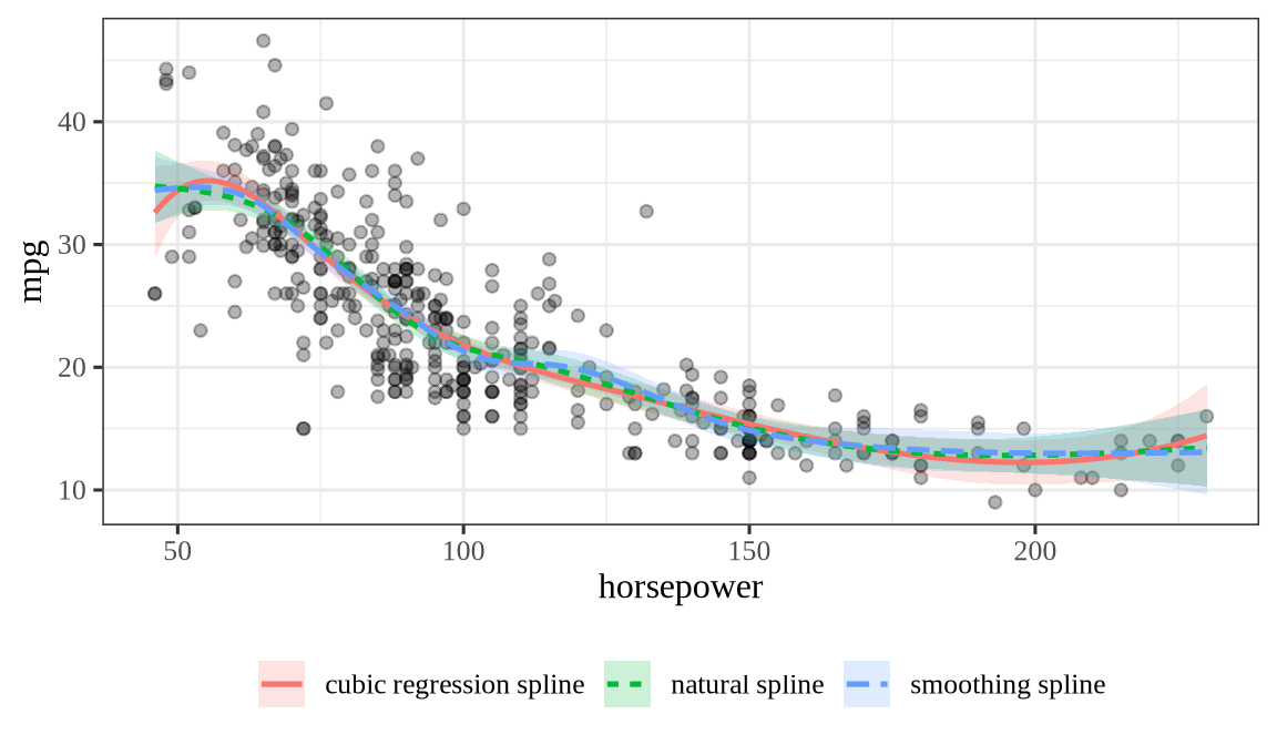
Kernel smoothing and local regression estimate the curve at each point from nearby data instead of a global basis, and give fits like those above; splines are the form that adds up to a linear model, which makes them easy to fit and, as additive models do, to combine across several inputs.
4 Choosing the smoothing parameter
Exercise 6 (When is leave-one-out cross-validation cheap to approximate?)
Exercise 6 (When is leave-one-out cross-validation cheap to approximate?) For a linear smoother \(\hat{\vy} = S\vy\) the leave-one-out residual is \((y_i - \hat y_i) / (1 - S_{ii})\). Suppose every diagonal entry of \(S\) equals the same number, \(S_{ii} = c\) for all \(i\). Express \(c\) through the trace of \(S\).
Solution 6. Adding up the \(n\) equal diagonal entries gives \(\trf{S} = nc\), so \(c = \trf{S} / n\).
Exercise 7 (When is leave-one-out cross-validation cheap to approximate? (part 2))
Exercise 7 (When is leave-one-out cross-validation cheap to approximate? (part 2)) Use the setup of Exercise 6.
Write the leave-one-out sample mean squared error (sMSE) using only the ordinary residuals and \(\trf{S}\).
Solution 7. Substituting \(S_{ii} = \trf{S} / n\) into every leave-one-out residual gives
\[ \frac{1}{n} \sum_{i=1}^n \paren{\frac{y_i - \hat y_i}{1 - \trf{S}/n}}^2 = \frac{\frac{1}{n} \sum_{i=1}^n \paren{y_i - \hat y_i}^2}{\paren{1 - \trf{S}/n}^2}, \]
because the denominator no longer depends on \(i\) and comes out of the sum. Only the residual sum of squares and the trace remain, with no need for the individual \(S_{ii}\).
Definition 4 (Generalized cross-validation and restricted maximum likelihood)
Definition 4 (Generalized cross-validation and restricted maximum likelihood) For a linear smoother \(\hat{\vy} = S_\regpar \vy\) with smoothing parameter \(\regpar\), the generalized cross-validation (GCV) score replaces each diagonal entry \(S_{ii}\) in the leave-one-out formula by their average, \(\trf{S_\regpar}/n\):
\[ \mathrm{GCV}(\regpar) \eqdef \frac{\frac{1}{n} \sum_{i=1}^n \paren{y_i - \hat y_i}^2}{\paren{1 - \trf{S_\regpar}/n}^2}. \]
The trace \(\trf{S_\regpar}\) is the effective degrees of freedom of the fit. The estimate \(\hat\regpar\) minimizes \(\mathrm{GCV}(\regpar)\) [1, Ch. 7], [4], [6].
Restricted maximum likelihood (REML) chooses \(\regpar\) differently, by treating the penalty as a Gaussian prior on the spline coefficients and maximizing the likelihood of the data with those coefficients integrated out [7, Sec. 6.2], [8]. The mgcv fits in these notes use it, through method = "REML".
Example 5 (Choosing the smoothing parameter for the Auto data by GCV and by REML)
Example 5 (Choosing the smoothing parameter for the Auto data by GCV and by REML) Score the same grid of \(\regpar\) as Example 4 with \(\mathrm{GCV}\), and compare the minimizer with the leave-one-out choice. The REML fit uses R’s mgcv, so it appears only in the R tab.
def gcv(y, fitted, s_diag):
    # Mean squared residual, inflated by the squared fraction of degrees of freedom left over.
    n = len(y)
    return np.mean((y - fitted) ** 2) / (1 - s_diag.sum() / n) ** 2

gcv_py = []
for ll in log_lams:
    fit, s_diag = penalized_fit(N_sm, Omega_sm, y_sp, 10.0**ll)
    gcv_py.append(gcv(y_sp, fit, s_diag))
best_gcv_py = int(np.argmin(gcv_py))
print(log_lams[best_gcv_py], round(np.sqrt(gcv_py[best_gcv_py]), 3))
-1.5 4.317gcv <- function(y, fit) {
# Mean squared residual, inflated by the squared fraction of degrees of freedom left over.
mean((y - fit$fitted)^2) / (1 - sum(fit$s_diag) / length(y))^2
}
gcv_r <- sapply(log_lams, function(ll) {
gcv(y_sp, penalized_fit(N_sm, Omega_sm, y_sp, 10^ll))
})
best_gcv_r <- which.min(gcv_r)
round(c(log10_lambda = log_lams[best_gcv_r], root_gcv = sqrt(gcv_r[best_gcv_r])), 3)log10_lambda root_gcv
-1.500 4.317 df sp.s(x)
6.563 316.295 GCV picks \(\log_{10} \regpar =\) -1.5, against -1.25 for leave-one-out, with 8.8 effective degrees of freedom. The two choices are one grid step apart, as expected when the diagonal entries \(S_{ii}\) are close to their average, the case of Exercise 6. REML reports 6.6 effective degrees of freedom, intercept included, a smoother fit than the GCV choice; its penalty is scaled differently from the \(\regpar\) above, so compare the degrees of freedom and not the penalty values. GCV is more prone than REML to choosing a wiggly fit [7, Sec. 6.2], one reason the mgcv fits here use method = "REML". One data set does not settle which criterion is better in general.