# The Python chunks on this page import numpy and pandas; reticulate provisions them.# The Julia chunks run through JuliaCall.reticulate::py_require(c("numpy", "pandas"))# Which label Julia's argmax over a Dict of vote counts picks from a 2-2 tie.jl_tie <-function(a, b) { JuliaCall::julia_eval(sprintf("argmax(Dict(%d => 2, %d => 2))", a, b))}# Julia's printed form of an expression, as inline code.jl_code <-function(expr) {paste0("`", JuliaCall::julia_eval(paste0("repr(", expr, ")")), "`")}
Source
Adapted from Kameron Decker Harris’ 2022 weekly notes, and drawing on Logan Sizemore’s Spring 2025 lecture on decision trees. The Gini index and the reference on classification and regression trees are from the cited sources rather than from that lecture, which measures impurity by entropy alone.
A First Model and Generalization distinguished parametric models, which compress the training data into a fixed set of weights, from non-parametric ones. From here on we use the sharper version of the second definition: a model is non-parametric when its effective number of parameters grows with the size of the training set rather than being fixed in advance.
The most visible way to satisfy that is to keep the data around. K-nearest neighbors (KNN) and kernel smoothing do so [1]: neither has any parameters to speak of, so every prediction consults the training set directly. A decision tree does not store the data, but it is non-parametric under the growth definition, because a larger training set supports a deeper tree with more splits. Every model so far has been parametric except support vector machines, whose support set grows with the data — so by the growth definition they are non-parametric too, even though they are usually introduced alongside the parametric models.
Watch
Andrew Ng explains the difference between parametric and non-parametric algorithms, from 5:53[2], Lecture 3.
This chapter covers those three: K-nearest neighbors, kernel smoothing, and decision trees.
1 K-nearest neighbors
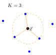
Take \(\vx_i\) with \(y_i \in \{0,1\}\) or \(y_i \in \reals\), and an integer parameter \(K\). Then
\[f(\vx) =
\begin{cases}
\text{most frequent label of the } K \text{ neighbors} & \textcolor{orange}{\text{classification}} \\[0.4em]
\displaystyle\sum_{i \in N_K(\vx)} \frac{y_i}{K} & \textcolor{orange}{\text{regression}}
\end{cases}\]
Either way the work is in finding the neighbors, and a brute-force search does it per query in \(\mathcal{O}(nd)\) to compute all \(n\) distances, plus \(\mathcal{O}(n \log K)\) to keep the smallest \(K\) of them. Nothing is done at training time at all.
The first step is to find the neighbors:
Order the training points by how far they are from \(\vx\),
There is nothing to fit, so the model is the training data itself plus one function that searches it. Three details of these implementations matter.
We compare distances squared and never take their square roots. The square root is monotone, so it cannot change which points come out nearest. Leaving it out saves \(n\) square roots on every query.
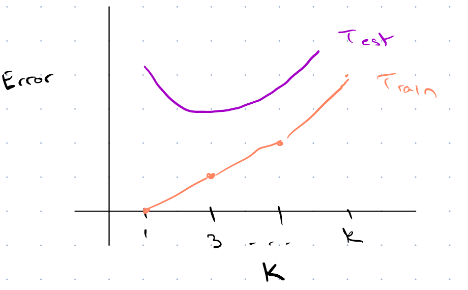
Finding the \(K\) smallest does not need a full sort. That \(\mathcal{O}(n \log K)\) is the cost of the obvious method: scan all \(n\) points while keeping a \(K\)-element heap. Here \(K\) is a hyperparameter that we fix independently of \(n\), so \(\log K\) is a constant. All three implementations below are therefore \(\mathcal{O}(n)\) as well, and none of them beats that bound in order. They differ in how much ordering they do along the way. Python’s argpartition only partitions around the \(K\)th element, which is \(\mathcal{O}(n)\) expected, and leaves the \(K\) it returns in no particular order. Julia’s partialsortperm also stops short of a full sort, but it does order the \(K\) it returns: partialsortperm([5,3,9,1,7,2], 1:3) returns [4, 6, 2], the positions of \(1\), \(2\) and \(3\), ascending. R’s order orders all \(n\), but not at \(\mathcal{O}(n \log n)\): its default method = "auto" dispatches to a radix sort for numeric input, which ?order documents as sorting “in linear time” and as outperforming the comparison methods. So the shorter call is not the slower one asymptotically. Timing it against an explicit method = "shell" at \(n = 50\,000\) — 200 calls each on five fresh rnorm vectors, under R 4.6.1 — puts the default ahead by a factor of \(3.4\) to \(3.8\). That is one machine and one \(n\); the asymptotics are the claim, and the ratio is only an illustration of them. Compared with the two calls that partition first, order costs a constant factor more, because it computes a full ordering that the query never reads past position \(K\).
Julia’s standard library has no mode, so we tally the vote by hand. StatsBase.mode replaces those four lines, but it needs a dependency the other two implementations do not.
Ties arise in two places: once among equidistant points at the edge of the neighbor set, and once among labels when the vote splits evenly. The two are not alike. The label tie is resolved identically in two of the three. Python votes with bincount, whose index is the label, and argmax returns the first maximum; R’s table orders its names by label and which.max likewise takes the first. Both give a \(2\)–\(2\) split to the lower label. Julia’s argmax also returns the first maximum, but the container here is a Dict, which iterates in hash order rather than key order — so which label is “first” depends on the label values themselves. On Julia 1.12.6, a \(2\)–\(2\) split between labels \(1\) and \(2\) goes to \(2\), and between \(3\) and \(7\) to \(7\), while \(0\) against \(1\) goes to \(0\), and the hash order, and with it the winner, can change from one Julia release to the next. Sorting the keys, or tallying into a vector indexed by label as Python does, makes the rule the same in all three. The tie is avoidable anyway, by taking \(K\) odd for two classes, and \(K = 15\) here. The neighbor tie is genuinely unspecified, can differ between languages and between runs, and is not avoidable.
import numpy as nprng = np.random.default_rng(0)n, K =500, 15X = rng.normal(size=(n, 2))y = (X[:, 0] + X[:, 1] >0).astype(int)def knn_classify(X, y, xq, K): d2 = np.sum((X - xq) **2, axis=1) # squared distance ranks the same nb = np.argpartition(d2, K -1)[:K] # the K smallest, in no orderreturn np.bincount(y[nb]).argmax()grid = np.array([[-1.0, -1.0], [0.0, 0.0], [1.5, 0.5]])print([int(knn_classify(X, y, xq, K)) for xq in grid])
[0, 0, 1]
set.seed(0)n <-500K <-15X <-matrix(rnorm(2* n), ncol =2)y <-as.integer(X[, 1] + X[, 2] >0)knn_classify <-function(X, y, xq, K) { d2 <-rowSums(sweep(X, 2, xq)^2) # squared distance ranks the same nb <-order(d2)[seq_len(K)] # order() sorts all n votes <-table(y[nb])as.integer(names(votes)[which.max(votes)])}grid <-rbind(c(-1, -1), c(0, 0), c(1.5, 0.5))print(apply(grid, 1, function(xq) knn_classify(X, y, xq, K)))
[1] 0 1 1
usingRandomRandom.seed!(0);n, K =500, 15;X =randn(n, 2);y =Int.(X[:, 1] .+ X[:, 2] .>0);functionknn_classify(X, y, xq, K) d2 =vec(sum((X .- xq') .^2, dims =2)) # squared distance ranks the same nb =partialsortperm(d2, 1:K) # the K smallest, and only those votes =Dict{Int,Int}()for l in y[nb] votes[l] =get(votes, l, 0) +1endreturnargmax(votes)end;grid = [-1.0-1.0; 0.00.0; 1.50.5];println([knn_classify(X, y, grid[i, :], K) for i in1:size(grid, 1)])
[0, 1, 1]
The three do not agree point for point, because each draws its own random data from its own generator — and they disagree at exactly one of the three queries, \((0, 0)\), which lies on the boundary \(x_1 + x_2 = 0\) the labels were drawn from. A query on the decision boundary is the one place where a different sample of neighbors ought to change the answer. So the disagreement shows the method behaving correctly, not one of the three implementations being wrong. They share the procedure and its cost: \(\mathcal{O}(nd)\) per query to compute the distances, plus the selection on top of that. Every one of them touches all \(n\) training points to answer a single question. That is the drawback of doing no training.
Watch
Weinberger introduces the \(k\)-nearest-neighbour classifier, from 35:37[5], Lecture 3.
Hastie and Tibshirani fit \(k\)-nearest neighbours in code in their Python lab[6].
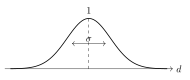
The bandwidth \(\bandwidth\) is the parameter: points at distance \(\le \bandwidth\) dominate.
Stores all the data in memory.
Biased depending on the density of the data.
Exercise 1 (Averaging versus fitting a line at the edge of the data)
Exercise 1 (Averaging versus fitting a line at the edge of the data) Three observations lie exactly on the line \(y = 2x\): \((x, y) = (0, 0), (1, 2), (2, 4)\). To estimate the regression function at the edge point \(x_0 = 0\), a kernel gives the three points the weights \(1, \tfrac12, \tfrac1{10}\). Compute the weighted average of the \(y_i\).
Solution 1. The weighted average is \((1 \cdot 0 + \tfrac12 \cdot 2 + \tfrac1{10} \cdot 4) / (1 + \tfrac12 + \tfrac1{10}) = 1.4 / 1.6 = 0.875\). It is too high, because every neighbor lies to the right of \(x_0 = 0\) and has a larger \(y\): the average is biased at an edge of the data.
Exercise 2 (Averaging versus fitting a line at the edge of the data (part 2))
Exercise 2 (Averaging versus fitting a line at the edge of the data (part 2)) Use the setup of Exercise 1.
Solution 2. The three points lie exactly on a line, so the weighted least squares line is that line whatever the weights are, and its intercept is \(0\).
Exercise 3 (Averaging versus fitting a line at the edge of the data (part 3))
Exercise 3 (Averaging versus fitting a line at the edge of the data (part 3)) Use the setup of Exercise 1.
Which one recovers \(f(0) = 0\), the weighted average or the intercept?
Solution 3. The intercept recovers \(f(0) = 0\), and the weighted average does not. Fitting a line at each query point removes this bias for any data on a line.
Definition 1 (Local linear regression) Let \(f(x) \eqdef \E{y \mid x}\) be the regression function. The local linear regression estimate of \(f(x_0)\) fits a line by weighted least squares around \(x_0\)[11],
Definition 2 (Span) The span of a local linear regression fit is the fraction \(\alpha\) of the data nearest to \(x_0\) that forms the neighborhood of \(x_0\).
Definition 3 (LOESS)LOESS[11], [12], [13] is local linear regression that takes the neighborhood to be the fraction \(\alpha\) (the span) of the data nearest to \(x_0\), and the tricube weights
Example 1 (LOESS for the Auto data) Estimate the mean miles per gallon, mpg, of cars at horsepower 100 in the Auto data [14] with spans \(0.3\) and \(0.75\):
import numpy as npimport pandas as pdauto_lo = pd.read_csv("data/auto.csv").dropna(subset=["horsepower"])x_lo = auto_lo["horsepower"].to_numpy(float)y_lo = auto_lo["mpg"].to_numpy(float)def local_linear(x0, x, y, span):# Neighborhood: the m points nearest x0; d is the distance to the farthest.# The same count as R's loess: floor(n * span + 1e-5). m =int(np.floor(span *len(x) +1e-5)) dist = np.abs(x - x0) d = np.sort(dist)[m -1]# Tricube weights, zero outside the neighborhood. w = np.where(dist < d, (1- (dist / d) **3) **3, 0.0)# Weighted least squares on (1, x - x0); the intercept is the estimate at x0. X = np.column_stack([np.ones_like(x), x - x0]) beta = np.linalg.solve(X.T @ (w[:, None] * X), X.T @ (w * y))return beta[0]for span in [0.3, 0.75]:print(span, round(local_linear(100.0, x_lo, y_lo, span), 3))
0.3 21.097
0.75 22.328
auto_lo <-read.csv("data/auto.csv")auto_lo <- auto_lo[!is.na(auto_lo$horsepower), ]# degree = 1 is a local line; surface = "direct" fits at the query point instead of interpolating.loess_at_100 <-sapply(c(0.3, 0.75), function(span) { fit <-loess(mpg ~ horsepower, data = auto_lo, span = span, degree =1,family ="gaussian", surface ="direct")predict(fit, data.frame(horsepower =100))})round(setNames(loess_at_100, c("0.3", "0.75")), 3)
   0.3   0.75
21.097 22.328
Both languages give the same estimates, 21.10 mpg for span \(0.3\) and 22.33 mpg for span \(0.75\), since the Python function implements the weights of Definition 3 directly. The wider neighborhood averages over cars with a wider range of horsepower, so it smooths over more of the curvature in the relationship.
Watch
Andrew Ng introduces locally weighted regression, from 5:38[2], Lecture 3.
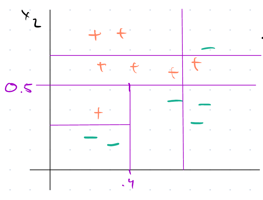
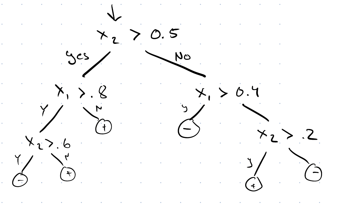
A decision tree partitions the input space into rectangles aligned with the axes. The number of nodes, that is of comparisons, measures the complexity of the tree, and a complex tree overfits.
The parts have names. The topmost node is the root; an internal node, which holds a comparison between one feature and one threshold, is a decision node; a terminal node, which holds a prediction, is a leaf. Applying a decision node’s comparison to send each point down one branch or the other is a split.
Goal:
Keep the tree as compact as possible.
Make the leaves pure.
Finding the optimal tree is NP-hard, so instead we greedily minimize the “impurity” of each split.
The University of Washington’s CSE 446 slides cover trees[9], Lecture 15.
3.1 Measuring impurity
The word “impurity” above is central to the algorithm, so we define it here. A node holding points of one class only is pure; a node holding an even mix of every class is as impure as a node can be. Two standard measures capture exactly this.
Entropy comes from information theory. An outcome of probability \(p\) carries \(-\log_2 p\) bits of surprisal: large when the outcome was unlikely, and zero when it was certain. Predicting heads on a single toss of a fair coin and being right is worth one bit; predicting ten heads in a row and being right is worth \(10\) bits. The population average of the surprisals, weighted by the probabilities themselves, is the entropy[19]:
\[H(S) = -\sumto{k}{C} p_k \log_2 p_k\]
where \(p_k\) is the fraction of the points in the set \(S\) that carry class \(k\), and \(0 \log_2 0\) is read as \(0\). It is zero when one class holds all the mass — there is nothing left to transmit — and largest, at \(\log_2 C\), when the classes are evenly split. So it measures impurity directly: the entropy of a node is the number of bits per point you would still have to send to resolve the labels once the reader knows which leaf a point fell into.
Here are three example nodes. A node holding \(10\) points of each of two classes has \(H = 1\) bit, the worst possible. A node holding \(10\) and \(4\) has \(H = 0.863\). A node holding \(10\) and \(0\) has \(H = 0\).
Gini impurity is the other standard choice:
\[G(S) = 1 - \sumto{k}{C} p_k^2\]
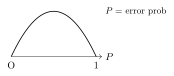
It is the probability that two points drawn independently from \(S\) carry different labels — equivalently, the error rate you would get by labeling a point at random from \(S\)’s own class proportions. It agrees with entropy at both ends, zero for a pure node and largest for an even mix, and differs only mildly in between, so the choice between the two rarely changes the tree that comes out. Entropy is the criterion of Quinlan’s ID3 [20]; Gini is the default in the classification and regression tree procedure of Breiman, Friedman, Olshen and Stone [21].
Watch
Weinberger builds decision trees from purity functions, from 14:43[5], Lecture 29.
A split sends the points of \(S\) into \(B\) branches \(S_1, \dots, S_B\) — \(B = 2\) for a yes-or-no comparison on one feature. Score it by how much impurity it removes. The impurity left afterwards is each branch’s impurity weighted by the share of the points that landed in it, and the information gain is the difference, which is the mutual information between a point’s branch and its class:
The weighted sum stops the greedy rule from being misled. Separating one point into its own branch makes that branch perfectly pure, but it arrives with weight \(1/|S|\) and leaves the other branch almost exactly as impure as the parent was, so the gain is negligible. The rule rewards a split for purifying a large share of the data, not for purifying something.
Growing the tree is then a loop: at each leaf, try every feature and every valid threshold, compute the gain for each candidate, keep the largest, and recurse on the branches it creates.
Example 2 (Comparing two candidate splits) Take \(16\) patients, \(8\) with a positive test and \(8\) with a negative one, described by two measurements \(x_1\) and \(x_2\). The root holds an even split, so \(H = 1\) bit. Consider two candidate splits:
split
branch
positive
negative
\(H\)
\(x_1 \leq 3\)
yes
\(3\)
\(0\)
\(0\)
no
\(5\)
\(8\)
\(0.961\)
\(x_2 \leq 1\)
yes
\(6\)
\(2\)
\(0.811\)
no
\(2\)
\(6\)
\(0.811\)
The first leaves \(\tfrac{3}{16}(0) + \tfrac{13}{16}(0.961) = 0.781\) bits, for a gain of \(0.219\). The second leaves \(\tfrac{8}{16}(0.811) + \tfrac{8}{16}(0.811) = 0.811\) bits, for a gain of \(0.189\). The first wins and becomes the root.
The winner is not the more balanced split. It carves off a perfectly pure branch, but only a small one, and still beats a split that makes both branches fairly pure: a pure branch removes all of its own impurity, and its small weight is the price. A split that purified only a single point would lose, because its weight would be too small to matter.
Watch
The CS229 lecture on trees formulates the splits, from 0:54, and compares split criteria, from 8:07[2], Lecture 9.
Exercise 4 (Compute the entropy of a skewed distribution)
Exercise 4 (Compute the entropy of a skewed distribution) A node holds points of four classes, in the proportions \(p = (\tfrac{1}{2}, \tfrac{1}{4}, \tfrac{1}{8}, \tfrac{1}{8})\). Compute its entropy \(H\) in bits, by hand.
import numpy as npdef entropy_py(p):# Entropy in bits of a vector of class proportions; terms with p = 0# are dropped, since 0 * log2(0) is read as 0. p = np.asarray(p, dtype=float) p = p[p >0]returnfloat(-np.sum(p * np.log2(p)))entropy_py([1/2, 1/4, 1/8, 1/8])
1.75
entropy_bits <-function(p) {# Entropy in bits of a vector of class proportions; terms with p = 0# are dropped, since 0 * log2(0) is read as 0. p <- p[p >0]-sum(p *log2(p))}entropy_bits(c(1/2, 1/4, 1/8, 1/8))
[1] 1.75
The code agrees with the hand calculation: \(H =\) 1.75 bits.
Exercise 5 (Compare with the uniform distribution)
Exercise 5 (Compare with the uniform distribution) Now take the same four classes in equal proportions, \(p = (\tfrac{1}{4}, \tfrac{1}{4}, \tfrac{1}{4}, \tfrac{1}{4})\). Compute \(H\).
Solution 7. With equal proportions every class is equally likely, so a reader who knows only which node a point fell into has no better guess than any other, and needs the full \(\log_2 4 = 2\) bits to name the label. In the skewed node the reader can bet on the common class, so the node is less impure. No distribution over four classes has more than \(\log_2 4\) bits, the entropy of the even split.
Exercise 8 (Compute the entropy at the root of a small tree)
Exercise 8 (Compute the entropy at the root of a small tree) A training set holds all eight combinations of three binary features \(x_1, x_2, x_3 \in \{0, 1\}\), labeled by the rule \(y = 1\) if both \(x_1 = 1\) and \(x_2 = 1\), and \(y = 0\) otherwise. The feature \(x_3\) plays no part in the rule.
\(x_1\)
\(x_2\)
\(x_3\)
\(y\)
0
0
0
0
1
0
0
0
0
1
0
0
1
1
0
1
0
0
1
0
1
0
1
0
0
1
1
0
1
1
1
1
What is the entropy of the labels at the root, before any split?
# All eight combinations of the three features, with the AND label.and_data <-expand.grid(x1 =0:1, x2 =0:1, x3 =0:1)and_data$y <-as.integer(and_data$x1 ==1& and_data$x2 ==1)# Entropy in bits of the labels in a node.node_entropy <-function(y) { p <-table(y) /length(y)-sum(p *log2(p))}node_entropy(and_data$y)
[1] 0.8112781
Code and hand calculation agree: \(H(S) =\) 0.811 bits.
Exercise 9 (Choose the first split by information gain)
Exercise 9 (Choose the first split by information gain) For the data of Exercise 8, compute the information gain of splitting on each of \(x_1\), \(x_2\) and \(x_3\).
Solution 9. Splitting on \(x_1\) sends four points to each branch. The branch \(x_1 = 0\) holds only \(y = 0\), so \(H = 0\). The branch \(x_1 = 1\) holds two points of each label, so \(H = 1\). The weighted remainder is \(\tfrac{4}{8}(0) + \tfrac{4}{8}(1) = 0.5\), and
The rule is symmetric in \(x_1\) and \(x_2\), so \(\mathrm{IG}(S, x_2) = 0.311\) too.
Splitting on \(x_3\) sends four points to each branch, and each branch holds one point with \(y = 1\) out of four. Both branches have \(H = 0.811\), the same as the root, so the remainder is \(0.811\) and \(\mathrm{IG}(S, x_3) = 0\).
# Information gain of splitting the AND data on one binary feature:# the root entropy minus the branch entropies, weighted by branch size.info_gain <-function(data, feature) { branches <-split(data$y, data[[feature]]) weights <-sapply(branches, length) /nrow(data)node_entropy(data$y) -sum(weights *sapply(branches, node_entropy))}sapply(c("x1", "x2", "x3"), info_gain, data = and_data)
       x1        x2        x3
0.3112781 0.3112781 0.0000000
Exercise 10 (Choose the first split by information gain (part 2))
Exercise 10 (Choose the first split by information gain (part 2)) Use the setup of Exercise 9.
Which feature, or features, would the greedy rule split on first?
Solution 10. Features\(x_1\) and \(x_2\) tie, each with a gain of 0.311 bits, so the greedy rule may split on either first. The irrelevant feature\(x_3\) gains nothing.
Solution 12. The branch \(x_1 = 1\) holds four points, two of each label, so its entropy is \(1\) bit. Splitting it on \(x_2\) gives two pure branches: \(x_2 = 0\) holds only \(y = 0\) and \(x_2 = 1\) holds only \(y = 1\). The remainder is \(0\), so the gain is the full \(1\) bit. Splitting it on \(x_3\) leaves each branch with one point of each label, so the remainder is \(1\) and the gain is \(0\).
# Gains inside the x1 = 1 branch, for the two features still available.branch <- and_data[and_data$x1 ==1, ]sapply(c("x2", "x3"), info_gain, data = branch)
Solution 13. Splitting on \(x_2\) inside the \(x_1 = 1\) branch finishes a tree with these leaves: \(y = 0\) when \(x_1 = 0\), \(y = 0\) when \(x_1 = 1\) and \(x_2 = 0\), and \(y = 1\) when \(x_1 = 1\) and \(x_2 = 1\).
Solution 15. That is the rule \(y = x_1 \wedge x_2\), so it classifies all eight points correctly, and it ignores \(x_3\), as the greedy rule never rewarded a split on it.
3.3 Regression trees
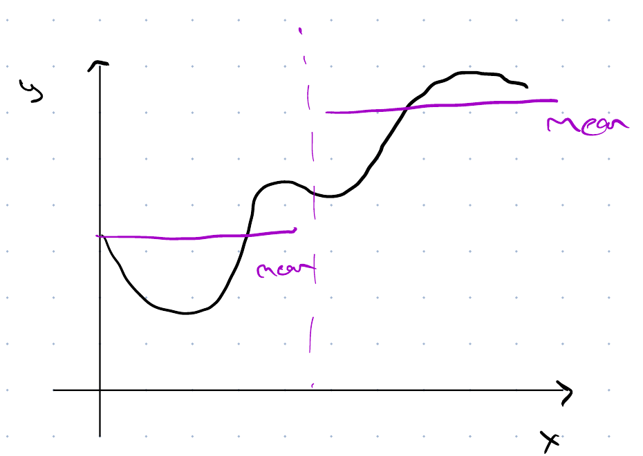
The same procedure fits numeric targets once we change the impurity measure. A leaf predicts the sample mean of the training targets it holds,
\[\hy_S = \frac{1}{|S|}\sum_{i \in S} y_i\]
so we measure a node’s impurity by how far its targets spread around that sample mean:
and a regression tree splits to maximize it. Because the leaf predicts the sample mean, \(|S|\,V(S)\) is exactly the squared error that leaf would incur, so maximizing variance reduction is minimizing training squared error one split at a time.
Nothing so far says when to stop, and the greedy rule will not stop on its own. It can keep splitting until every leaf holds a single point, at which stage the training error is zero and the tree has memorized the data rather than learned from it.
Two conditions end the recursion naturally: every leaf is pure, so no split can gain anything; or no candidate split gains enough to justify the extra depth. The first is reachable on any dataset without contradictory labels, and reaching it is the failure mode rather than the goal.
So we limit the growth deliberately instead, with one or both of two simple controls:
a maximum depth, capping how many comparisons any prediction can involve
a minimum number of points required in a leaf, or required in a node before it may be split at all
Both say the same thing from opposite directions — do not create a region so small that the points inside it are as likely to be noise as signal — and both are hyperparameters, which we choose by the procedure of Model Selection rather than from the data. Both encode Occam’s razor, the principle that asks for the simplest hypothesis that fits the observations. For a tree, the simplest hypothesis is the smallest tree.
CART stands for Classification And Regression Trees.
Handles discrete and continuous features.
Handles classification and regression with the same recursion, changing only the impurity measure.
Captures non-linear structure, because the regions are assembled by recursive cuts rather than described by one global function.
Overfits.
Does not need to store all the data, unlike KNN and kernel smoothing.
Fast.
Interpretable — but not really.
Subject to the curse of dimensionality.
The interpretability bullet needs explanation, because trees are usually promoted for it. A single fitted tree genuinely is as readable as a model gets: we can follow any prediction down the tree and report it as the few comparisons that produced it. The reservation concerns what that readability entitles you to conclude. A deep tree’s path is long enough that following it is no longer an explanation. The greedy rule commits to one split before considering what comes below, so a small change to the data can change an early split and alter everything under it. And two correlated features compete for the same split, so a feature’s absence from the tree is not evidence that it did not matter — only that the greedy rule chose its rival first.
W. S. Cleveland, “Robust locally weighted regression and smoothing scatterplots,”Journal of the American Statistical Association, vol. 74, no. 368, pp. 829–836, 1979, doi: 10.1080/01621459.1979.10481038.
[13]
W. S. Cleveland and S. J. Devlin, “Locally weighted regression: An approach to regression analysis by local fitting,”Journal of the American Statistical Association, vol. 83, no. 403, pp. 596–610, 1988, doi: 10.1080/01621459.1988.10478639.
[14]
G. James, D. Witten, T. Hastie, and R. Tibshirani, An introduction to statistical learning with applications in R, 2nd ed. Springer, 2021. Available: https://www.statlearning.com/
C. E. Shannon, “A mathematical theory of communication,”Bell System Technical Journal, vol. 27, no. 3, pp. 379–423, 1948, doi: 10.1002/j.1538-7305.1948.tb01338.x.
[20]
J. R. Quinlan, “Induction of decision trees,”Machine Learning, vol. 1, no. 1, pp. 81–106, 1986, doi: 10.1007/BF00116251.
[21]
L. Breiman, J. H. Friedman, R. A. Olshen, and C. J. Stone, Classification and regression trees. Belmont, CA: Wadsworth, 1984.
T. Hastie, R. Tibshirani, and J. Friedman, The elements of statistical learning: Data mining, inference, and prediction, 2nd ed. Springer, 2009. Available: https://hastie.su.domains/ElemStatLearn/