Ensemble Methods
Last modified: 2026-10-25
Source
Adapted from Logan Sizemore’s Spring 2025 lectures on bagging, random forests and boosting.
Non-Parametric Models ends by listing what is wrong with a decision tree: it overfits. A shallow tree cannot partition the input space finely enough and underfits. A deep one makes a separate region for each noisy point and overfits. The depth that balances the two is rarely deep enough to represent the boundary we wanted. Trees are fast, they handle mixed feature types, and they are about as interpretable as a model gets. On their own, however, they are usually beaten by almost anything else.
Ensembling fixes this. Rather than fitting one model, fit many and combine them [1]. Two strategies do this in opposite ways, and this chapter compares them:
Bagging (short for bootstrap aggregating) fits many models independently and averages them, to reduce variance
Boosting fits many models sequentially, each correcting its predecessor, to reduce bias [2]
Watch
The CS229 lecture on trees ends with ensemble methods, from 52:53 [3], Lecture 9.
Read
GeeksforGeeks explains ensemble learning [4].
1 Bagging
Bagging — bootstrap aggregating, from Breiman [5] — borrows a basic fact about sample means [6]. The sample mean of several independent measurements of the same quantity varies less than any single one of them. Bagging applies that to predictions: fit the model several times, and average what the copies predict.
There is only one training set, so we cannot collect fresh ones. The bootstrap manufactures stand-ins for them instead.
1.1 The bootstrap
Draw \(n\) points from the training set with replacement. The result is a training set of the original size that differs from it: some points appear twice or more, and some do not appear at all
Repeat \(B\) times to get \(B\) bootstrap samples, and fit a deep tree to each
To predict, average the \(B\) predictions (regression) or take the majority vote (classification):
\[\hat{f}_{\text{bag}}(x) = \frac{1}{B}\sumto{b}{B} \hat{f}^{*b}(x)\]
- A given training point is left out of a given bootstrap sample with probability
\[\paren{1 - \frac{1}{n}}^{n} \;\xrightarrow[n \to \infty]{}\; e^{-1} \approx 0.368\]
- so each bootstrap sample contains about \(63.2\%\) of the distinct training points. That figure comes up again in Section 1.3, because the other \(36.8\%\) turn out to be useful
Watch
Starmer explains the bootstrap [7].
Read
GeeksforGeeks explains the bootstrap [8].
1.2 Why averaging helps, and how much
If the \(B\) trees were independent, each with variance \(\varpar\), the sample average would have variance \(\varpar / B\) — and we could drive it to zero by taking \(B\) large enough
They are not independent. Each tree learns from an overlapping sample of the same data, so the trees make correlated errors. With pairwise correlation \(\corpar\), the variance of the sample average is
\[\corpar\,\varpar + \frac{1 - \corpar}{B}\,\varpar \tag{1}\]
The second term vanishes as \(B\) grows, but the first does not. Adding trees cannot reduce the variance below \(\corpar\varpar\), and the similarity of the trees to each other sets that lower limit
This single expression explains the whole design of the next section. To do better than bagging you cannot add more trees — you have to make them less alike
Bagging reduces variance but leaves bias where it was, so an ensemble of stumps still underfits and an ensemble of unpruned trees can still overfit
1.3 Out-of-bag error
-
The \(36.8\%\) of points left out of each bootstrap sample are a validation set that needs no extra data:
For each training point \(x_i\), collect the trees whose bootstrap sample did not contain it — about \(37\%\) of them
Average those trees’ predictions for \(x_i\) and score that prediction against \(y_i\)
Average the resulting point-wise errors over the training set
This out-of-bag (OOB) error estimates generalization error without a held-out split and without refitting. We therefore often tune bagged models on OOB error rather than by cross-validation
1.4 Feature importance
A single tree can be read off the page; five hundred averaged trees cannot
Instead, we use an aggregate: for each feature, sum the impurity reduction achieved by every split on that feature, across every tree. Features that repeatedly gave large reductions rank high
Treat the ranking as a description of this fitted ensemble, not as a causal claim. Correlated features split the credit between them arbitrarily, and this particular measure is biased towards high-cardinality features, which offer more split points to try
Watch
- The CS229 lecture on ensembles covers bagging and random forests, from 1:00:10 [3], Lecture 9.
- Hastie and Tibshirani cover bagging [9], video 8.4, and fit tree ensembles in code in their Python lab.
- Weinberger teaches bagging, from 31:50 [10], Lecture 30.
Read
GeeksforGeeks explains:
Read
The University of Washington’s CSE 446 slides cover the bootstrap [13], Lecture 16.
1.5 Bagging on real data
Exercise 1 (Bagging trees for fuel economy)
Exercise 1 (Bagging trees for fuel economy) The Auto data of James et al. [14] give the fuel efficiency (mpg) of 392 cars, with seven other measurements of each car. Download auto.csv to load it in Python or R. Use every third car (the 1st, 4th, 7th, and so on) as test data and the other cars as training data, and predict mpg from cylinders, displacement, horsepower, weight, acceleration, year and origin.
Fit one fully grown regression tree to the training cars.
Solution 1.
    mpg  cylinders  displacement  ...  year  origin                       name
0  18.0          8         307.0  ...    70       1  chevrolet chevelle malibu
1  15.0          8         350.0  ...    70       1          buick skylark 320
2  18.0          8         318.0  ...    70       1         plymouth satellite

[3 rows x 9 columns]
cols = ["cylinders", "displacement", "horsepower", "weight",
"acceleration", "year", "origin"]
is_test_py = (np.arange(len(auto_py)) % 3 == 0)
train_py, test_py = auto_py[~is_test_py], auto_py[is_test_py]
def mean_ci_py(sq):
# A 95% confidence interval for the mean of the squared errors of the test cars,
# which are independent of the trees: the mean plus or minus t_crit standard errors.
n = len(sq)
half = stats.t.ppf(0.975, df=n - 1) * sq.std(ddof=1) / np.sqrt(n)
return sq.mean() - half, sq.mean() + half
single_py = DecisionTreeRegressor(random_state=0).fit(train_py[cols], train_py["mpg"])
sq_single_py = (single_py.predict(test_py[cols]) - test_py["mpg"].to_numpy()) ** 2
mse_single_py = sq_single_py.mean()
# sRMSE is the square root of the sMSE, and so are its interval's endpoints.
print("single tree sRMSE:", np.sqrt(mse_single_py).round(2),
np.round(np.sqrt(mean_ci_py(sq_single_py)), 2))single tree sRMSE: 3.9 [2.91 4.69]cols <- c("cylinders", "displacement", "horsepower", "weight",
"acceleration", "year", "origin")
is_test <- (seq_len(nrow(auto)) - 1) %% 3 == 0
train <- auto |>
dplyr::filter(!is_test) |>
dplyr::select(mpg, dplyr::all_of(cols))
test <- auto |>
dplyr::filter(is_test) |>
dplyr::select(mpg, dplyr::all_of(cols))
grow <- function(data) {
rpart(mpg ~ ., data = data,
control = rpart.control(minsplit = 2, cp = 0, xval = 0))
}
# The squared error of each test car, and a 95% confidence interval for their mean.
# The test cars are independent of the trees, so the mean of their squared errors
# is the test error, and its interval is the mean plus or minus t_crit standard errors.
sq_err <- function(pred) (pred - test$mpg)^2
mean_ci <- function(sq) {
half <- qt(0.975, df = length(sq) - 1) * sd(sq) / sqrt(length(sq))
c(lower = mean(sq) - half, upper = mean(sq) + half)
}
mse <- function(pred) mean(sq_err(pred))
sq_single <- sq_err(predict(grow(train), test))
mse_single <- mean(sq_single)
c(single_tree = sqrt(mse_single))single_tree
3.802932 The two languages grow trees with different algorithms and draw different bootstrap samples, so their printed errors differ. The numbers below are from the R run.
The single fully grown tree has a test sample root mean squared error (sRMSE) of 3.80 mpg, with a 95% confidence interval of [2.79, 4.60]. The sRMSE is the square root of the sample mean squared error, so it is in the units of mpg and not in squared mpg (why we report sRMSE). Each interval is the \(t\) interval for the sample mean of the test cars’ squared errors, the sample mean plus or minus 1.98 standard errors, with its endpoints square-rooted.
Exercise 2 (Bagging trees for fuel economy (part 2))
Exercise 2 (Bagging trees for fuel economy (part 2)) Use the setup of Exercise 1.
Bag \(B = 100\) fully grown trees, each fit to a bootstrap sample of the training cars.
Solution 2.
rng = np.random.default_rng(571)
preds_py = []
for _ in range(100):
    boot = train_py.iloc[rng.integers(0, len(train_py), len(train_py))]
    tree = DecisionTreeRegressor(random_state=0).fit(boot[cols], boot["mpg"])
    preds_py.append(tree.predict(test_py[cols]))
running_py = np.cumsum(preds_py, axis=0) / np.arange(1, 101)[:, None]
sq_bag_py = (running_py - test_py["mpg"].to_numpy()) ** 2
mse_bag_py = sq_bag_py.mean(axis=1)
print("100 bagged trees sRMSE:", np.sqrt(mse_bag_py[-1]).round(2),
      np.round(np.sqrt(mean_ci_py(sq_bag_py[-1])), 2))
100 bagged trees sRMSE: 2.95 [1.95 3.69]bagged_100
2.963071 Averaging \(100\) bootstrap trees gives a test sRMSE of 2.96 mpg ([1.96, 3.70]), which is 22% smaller than the single tree’s.
Exercise 3 (Bagging trees for fuel economy (part 3))
Exercise 3 (Bagging trees for fuel economy (part 3)) Use the setup of Exercise 1.
Plot the test sample mean squared error (sMSE) of the bagged average against the number of trees.
Solution 3. The error falls quickly over the first ten trees and then flattens, as Figure 1 shows.
Show code
library(ggplot2)
# One row per number of trees: the test sRMSE and its 95% confidence interval.
bag_df <- tibble::tibble(
  trees = 1:100, rmse = sqrt(mse_bag),
  lower = sqrt(ci_bag[, "lower"]), upper = sqrt(ci_bag[, "upper"])
)
single_ci <- sqrt(mean_ci(sq_single))
ggplot(bag_df, aes(trees, rmse)) +
  geom_ribbon(aes(ymin = lower, ymax = upper), alpha = 0.2) +
  geom_line(aes(linetype = "bagged average"), linewidth = 0.9) +
  geom_hline(aes(yintercept = sqrt(mse_single), linetype = "single tree")) +
  geom_hline(yintercept = single_ci, linetype = "dotted", colour = "grey40") +
  scale_linetype_manual(
    values = c("bagged average" = "solid", "single tree" = "dashed")
  ) +
  labs(x = "number of bagged trees", y = "test sRMSE (mpg)",
       linetype = NULL) +
  theme(legend.position = "bottom")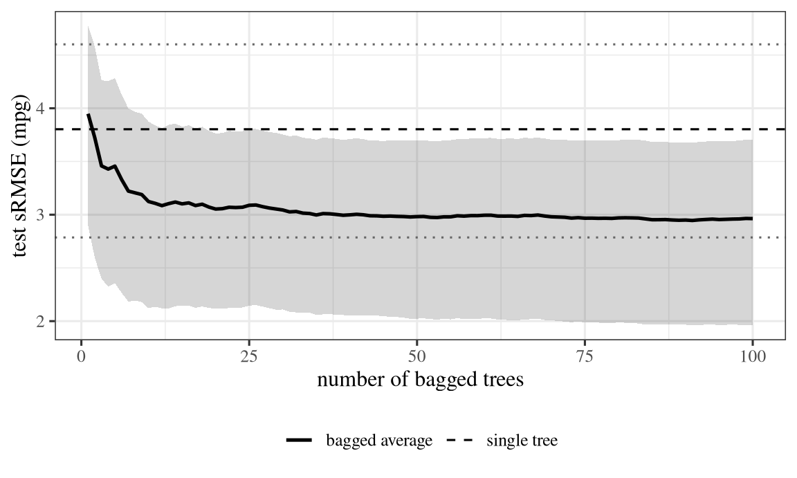
Exercise 4 (Bagging trees for fuel economy (part 4))
Exercise 4 (Bagging trees for fuel economy (part 4)) Use the setup of Exercise 1.
Compare the test sMSE of the bagged average with that of the single tree.
Solution 4.
# Both models predict the same test cars, so the 95% interval for the difference
# in their errors uses each car's difference in squared error.
print("single tree minus 100 bagged trees, mean squared error:",
      (mse_single_py - mse_bag_py[-1]).round(2),
      np.round(mean_ci_py(sq_single_py - sq_bag_py[-1]), 2))
single tree minus 100 bagged trees, mean squared error: 6.52 [ 2.81 10.23]The two models predict the same 131 test cars, so the better comparison is of each car’s difference in squared error: the single tree’s sMSE is larger by 5.7 mpg\(^2\) on average, with a 95% confidence interval of [2.1, 9.3]. These intervals reflect which test cars were drawn. They do not reflect which training cars were drawn, or which bootstrap samples, so a different split could move both errors.
2 Random forests
Bagged trees are correlated because each follows the same greedy rule on nearly the same data: if one feature is strongly predictive, every tree splits on it first, and the trees agree from the root down
-
A random forest breaks that agreement with a second source of randomness [15]. Bagging randomizes the rows; a random forest also randomizes the columns:
Fit each tree to its own bootstrap sample, as in bagging
At each split, draw a random subset of \(m\) features and choose the best split from that subset only
The strongly predictive feature is now unavailable in a fraction of splits, so the trees use other features and diverge. That lowers \(\corpar\) and therefore lowers the lower limit in Equation 1
The trade is visible in the same expression: restricting the split candidates makes each individual tree slightly worse, raising \(\varpar\). The trade helps as long as \(\corpar\) falls faster than \(\varpar\) rises, and for trees it usually does
-
The main settings to choose in advance, where \(\ninputvars\) is the number of features:
Name What it controls Typical default n_estimatorsnumber of trees \(B\) as many as you can afford max_featuresfeatures per split \(m\) \(\sqrt{\ninputvars}\) (classification), \(\ninputvars/3\) (regression) max_depthcomplexity of each tree unlimited \(B\) is not a complexity parameter and does not need tuning against a validation set: the variance expression is monotone decreasing in \(B\), so more trees never overfit, they only cost time
Watch
- Weinberger teaches random forests [10], Lecture 31.
- Starmer explains building, using and evaluating random forests [16].
Read
GeeksforGeeks explains random forests [17].
Read
The University of Washington’s CSE 446 slides cover random forests [13], Lecture 17.
3 Boosting
Bagging and random forests reduce variance by averaging models that each see the whole problem. If every tree finds the same examples hard, averaging them changes nothing — the error is bias, and averaging does not touch bias
Boosting addresses that case. It fits models sequentially and aims each new model at what the current ensemble gets wrong
We keep the base learners (the individual models we combine) deliberately weak, usually shallow trees. The smallest is a stump: one split, two leaves. A stump alone does little better than guessing. Boosting needs nothing more of it, because its guarantee holds for any learner that beats chance by a margin on the weighted data [18]
3.1 AdaBoost
AdaBoost, short for adaptive boosting, made boosting practical [18], [19]. Here the labels are \(y_i \in \{-1, +1\}\).
Initialize equal weights \(w_i^{(1)} = 1/n\) on every training point
-
For \(t = 1, \dots, T\):
Fit a weak learner \(h_t\) to the training set weighted by \(w^{(t)}\)
Compute its weighted error
\[\wterr_t = \sumin w_i^{(t)} \,\mathbf{1}\sb{y_i \neq h_t(x_i)}\]
- Compute the learner’s coefficient
\[\votewt_t = \tfrac{1}{2}\lnf{\frac{1 - \wterr_t}{\wterr_t}}\]
- Reweight and renormalize so the weights again sum to one
\[w_i^{(t+1)} \;\propto\; w_i^{(t)} \expf{-\votewt_t\, y_i\, h_t(x_i)}\]
Predict with the weighted vote of the whole sequence
\[H(x) = \operatorname{sign}\paren{\sumto{t}{T} \votewt_t h_t(x)}\]
Three facts follow from those formulas:
\(\votewt_t\) is large when \(\wterr_t\) is small and goes to zero as \(\wterr_t \to 1/2\). An accurate learner gets a large weight in the vote, and a random-guessing learner gets none
The exponent \(-\votewt_t y_i h_t(x_i)\) is negative when \(h_t\) got point \(i\) right and positive when it got it wrong, so correct points lose weight and misclassified points gain it. We fit the next learner to a dataset that emphasizes exactly what the last one missed
\(\wterr_t > 1/2\) makes \(\votewt_t\) negative. This is not a failure: a learner that is reliably wrong is a useful learner with its sign reversed
3.2 Gradient boosting
AdaBoost’s reweighting is specific to a particular loss. Gradient boosting generalizes the idea to any differentiable loss [22]. We state the generalization for squared error, where it is easiest to state.
- Initialize with the constant that minimizes the loss — for squared error, the sample mean of the training labels:
\[F_0(x) = \bar{y}\]
-
For \(t = 1, \dots, T\):
- Compute the residuals of the current model
\[r_i^{(t)} = y_i - F_{t-1}(x_i)\]
Fit a shallow tree \(h_t\) to the residuals, not to \(y\)
Add it to the model, shrunk by a learning rate \(\shrinkage\)
\[F_t(x) = F_{t-1}(x) + \shrinkage\, h_t(x)\]
We keep the trees shallow, typically three to six levels. Depth is the main way gradient boosting overfits: with deep enough trees, the first few drive the training residuals to zero and every later tree fits noise
The learning rate \(\shrinkage\) (commonly \(0.1\) or smaller) makes the ensemble additive rather than greedy. Small \(\shrinkage\) needs more trees and generalizes better — \(\shrinkage\) and \(T\) trade against each other, so we should tune them together
3.3 Why “gradient”
- For squared error \(L = \tfrac{1}{2}(y - F(x))^2\), the derivative with respect to the model’s own output is
\[ \begin{aligned} \frac{\partial L}{\partial F(x_i)} &= -(y_i - F(x_i)) \\ &= -r_i \end{aligned} \]
So the residual is the negative gradient of the loss with respect to the prediction, and the update \(F_t = F_{t-1} + \shrinkage h_t\) is a gradient descent step — in the space of functions rather than the space of parameters
Replace squared error with another differentiable loss and the procedure is unchanged: fit each tree to the negative gradient of that loss. Squared error is the case where the negative gradient happens to be the familiar residual
The connection is more useful than it is elegant. It brings in everything known about gradient descent from Gradient Descent — what the learning rate does, why shrinkage acts as regularization, when the procedure converges
Watch
- The CS229 lecture on ensembles introduces boosting, from 1:11:08 [3], Lecture 9.
- Starmer explains gradient boosting [23] and works through the details for regression [24].
Read
GeeksforGeeks explains gradient boosting [25].
4 Bagging against boosting
| Bagging / random forest | Boosting | |
|---|---|---|
| Models fitted | independently, in parallel | sequentially, each on the last’s errors |
| Base learner | deep, low-bias, high-variance | shallow, high-bias, low-variance |
| Chiefly reduces | variance | bias |
| More models | never overfits, just costs time | can overfit; \(T\) needs tuning |
| Parallelizes | trivially | not across \(t\) |
| Built-in validation | out-of-bag error | none |
The two are complementary rather than competing. A random forest is the safer default — it has one hyperparameter that matters, and running it longer cannot make it worse. A carefully tuned gradient-boosted ensemble usually predicts best on tabular data, but it needs a tuning budget.
Read
GeeksforGeeks compares bagging and boosting [26].
5 Ensembling neural networks
The averaging behind bagging is not specific to trees. Training the same network several times from different initializations and averaging the predictions reliably improves both accuracy and calibration, for the same variance-reduction reason
Dropout makes this affordable. During training, dropout zeroes each unit independently with probability \(1 - p\) on each forward pass, so every example flows through a different subnetwork
A network with \(n\) units has \(2^n\) possible subnetworks, and all of them share one set of weights. Training with dropout therefore trains a huge ensemble, and using the full network at the end approximates averaging it. The cost is that of a single network
-
Three details decide whether an implementation is correct:
We scale a kept unit’s output by \(1/p\) during training, so that the expected input to the next layer does not change with \(p\)
We switch dropout off when we predict. Every unit is active at test time, and we use the outputs as they are. (Some libraries do the opposite and rescale at test time instead of during training. The two conventions put the factor in different places but give the same trained model)
The letter \(p\) means opposite things in different sources. Here, and in the formulation that introduced dropout, \(p\) is the probability a unit is kept, so the scale factor is \(1/p\). PyTorch’s
nn.Dropouttakes \(p\) as the probability a unit is zeroed, and scales by \(1/(1-p)\). The mechanism is the same either way, but the letter is reversed, sonn.Dropout(0.2)is this section’s \(p = 0.8\)
6 AdaBoost in code
The code in this section runs AdaBoost with decision stumps on a one-dimensional problem that no single stump can solve: the label is \(+1\) when \(|x| > 1\) and \(-1\) otherwise, so the positive class lies on both sides of the negative one. The best possible single stump misclassifies three of the nine points. Look at the training error of the weighted vote as rounds accumulate.
import numpy as np


def best_stump(x, y, w):
    """Weighted-error-minimizing stump over thresholds and both polarities."""
    best = None
    for threshold in np.unique(x):
        for polarity in (1, -1):
            pred = np.where(polarity * (x - threshold) >= 0, 1.0, -1.0)
            err = w[pred != y].sum()
            if best is None or err < best[0]:
                best = (err, threshold, polarity)
    return best


def adaboost(x, y, rounds):
    w = np.full(len(x), 1 / len(x))
    stumps = []
    for _ in range(rounds):
        err, threshold, polarity = best_stump(x, y, w)
        err = min(max(err, 1e-10), 1 - 1e-10)
        alpha = 0.5 * np.log((1 - err) / err)
        pred = np.where(polarity * (x - threshold) >= 0, 1.0, -1.0)
        w = w * np.exp(-alpha * y * pred)
        w = w / w.sum()
        stumps.append((alpha, threshold, polarity))
        margin = sum(a * np.where(p * (x - t) >= 0, 1.0, -1.0)
                     for a, t, p in stumps)
        print(len(stumps), round(err, 3),
              round(np.mean(np.sign(margin) != y), 3))


x = np.array([-3.0, -2.0, -1.5, -0.5, 0.0, 0.5, 1.5, 2.0, 3.0])
y = np.where(np.abs(x) > 1, 1.0, -1.0)
adaboost(x, y, 4)
1 0.333 0.333
2 0.25 0.333
3 0.167 0.0
4 0.2 0.0stump_predict <- function(x, threshold, polarity) {
ifelse(polarity * (x - threshold) >= 0, 1, -1)
}
best_stump <- function(x, y, w) {
best <- NULL
for (threshold in unique(x)) {
for (polarity in c(1, -1)) {
err <- sum(w[stump_predict(x, threshold, polarity) != y])
if (is.null(best) || err < best$err) {
best <- list(err = err, threshold = threshold, polarity = polarity)
}
}
}
best
}
adaboost <- function(x, y, rounds) {
w <- rep(1 / length(x), length(x))
margin <- rep(0, length(x))
for (step in seq_len(rounds)) {
fit <- best_stump(x, y, w)
err <- min(max(fit$err, 1e-10), 1 - 1e-10)
alpha <- 0.5 * log((1 - err) / err)
pred <- stump_predict(x, fit$threshold, fit$polarity)
w <- w * exp(-alpha * y * pred)
w <- w / sum(w)
margin <- margin + alpha * pred
cat(step, round(err, 3), round(mean(sign(margin) != y), 3), "\n")
}
}
x <- c(-3, -2, -1.5, -0.5, 0, 0.5, 1.5, 2, 3)
y <- ifelse(abs(x) > 1, 1, -1)
adaboost(x, y, 4)1 0.333 0.333
2 0.25 0.333
3 0.167 0
4 0.2 0 stump_predict(x, threshold, polarity) =
[polarity * (xi - threshold) >= 0 ? 1.0 : -1.0 for xi in x];
function best_stump(x, y, w)
best = nothing
for threshold in unique(x), polarity in (1, -1)
pred = stump_predict(x, threshold, polarity)
err = sum(w[pred .!= y])
if best === nothing || err < best[1]
best = (err, threshold, polarity)
end
end
best
end;
function adaboost(x, y, rounds)
w = fill(1 / length(x), length(x))
margin = zeros(length(x))
for r in 1:rounds
err, threshold, polarity = best_stump(x, y, w)
err = min(max(err, 1e-10), 1 - 1e-10)
alpha = 0.5 * log((1 - err) / err)
pred = stump_predict(x, threshold, polarity)
w = w .* exp.(-alpha .* y .* pred)
w = w ./ sum(w)
margin = margin .+ alpha .* pred
println(r, " ", round(err, digits = 3), " ",
round(sum(sign.(margin) .!= y) / length(y), digits = 3))
end
end;
x = [-3.0, -2.0, -1.5, -0.5, 0.0, 0.5, 1.5, 2.0, 3.0];
y = [abs(xi) > 1 ? 1.0 : -1.0 for xi in x];
adaboost(x, y, 4)1 0.333 0.333
2 0.25 0.333
3 0.167 0.0
4 0.2 0.0The first stump’s weighted error is \(1/3\) — the best a single split can manage on this data — and the ensemble’s training error reaches zero within a few rounds. We keep err away from \(0\) and \(1\) before taking the logarithm: a weak learner that happens to be perfect on the current weights would otherwise send \(\votewt_t\) to infinity.
7 Further reading
Breiman [5] — bagging, and why averaging reduces variance
Breiman [29] — decorrelating the trees as well as resampling
Schapire [30] — the first boosting algorithm, seven years before AdaBoost, and the proof that weak learnability implies strong
Freund and Schapire [18] — AdaBoost, and the decision-theoretic argument behind the weight update
Friedman [31] — the function-space gradient-descent view
Zhou [32], Tree-Based Methods — slides that go from a single tree through bagging and random forests to AdaBoost and gradient boosting, with code in both R and Python
Hastie et al. [33], Chapters 10 and 15
Watch
Section 8.2 of An Introduction to Statistical Learning covers bagging, random forests and boosting. The Data Science Learning Community’s book clubs discuss its Chapter 8 in recorded meetings:
- the R book club, in part 1 and part 2 [34];
- the Python book club, in a meeting on Chapters 7 and 8 and one on Chapter 8 [35].