Last modified: 2026-10-25
Source
Written for these notes, following Hastie and Tibshirani’s Generalized Additive Models [1] for the definitions and backfitting, and Wood’s Generalized Additive Models: An Introduction with R [2] for practice. James, Witten, Hastie and Tibshirani [3, Ch. 7] give the short version.
Splines fit a flexible curve to one predictor. With several predictors, a flexible function of all of them at once needs far more data, because the number of possible interactions grows quickly. An additive model keeps the interpretability of a linear model, one curve per predictor, and lets each curve have its own shape.
Exercise 1 (What a linear model assumes about each predictor)
Exercise 1 (What a linear model assumes about each predictor) A linear model for mpg from horsepower and weight is \(\text{mpg} = \beta_0 + \beta_1\, \text{horsepower} + \beta_2\, \text{weight} + \noise\). Name two things this model assumes about how horsepower affects mpg.
Solution 1. The model assumes that the effect is linear: each extra unit of horsepower changes the predicted mpg by the same \(\beta_1\), wherever horsepower starts. It also assumes that the effect is additive: the change does not depend on weight, because the horsepower and weight terms are simply added.
Exercise 2 (What a linear model assumes about each predictor (part 2))
Exercise 2 (What a linear model assumes about each predictor (part 2)) Use the setup of Exercise 1.
Which of the two does a spline in horsepower relax?
Solution 2. Replacing \(\beta_1\, \text{horsepower}\) by a spline in horsepower relaxes linearity and keeps additivity.
Exercise 3 (What a linear model assumes about each predictor (part 3))
Exercise 3 (What a linear model assumes about each predictor (part 3)) Use the setup of Exercise 1.
Which of the two would still need a new feature, such as a product of the two predictors?
Solution 3. Letting the effect of horsepower depend on weight is an interaction, which needs a new feature such as the product. An additive model keeps the second assumption and drops the first, for every predictor at once [4].
Definition 1 (Component function)
Definition 1 (Component function) A component function is a smooth function \(f\) of one predictor \(x\) with \(\E{f(x)} = 0\).
Definition 2 (Additive model)
Definition 2 (Additive model) An additive model for a response \(y\) and predictors \(x_1, \dots, x_p\) is
\[ y = \beta_0 + f_1(x_1) + \dots + f_p(x_p) + \noise, \]
where each \(f_j\) is a component function (Definition 1) [4].
Remark 1 (Why component functions are centered)
Remark 1 (Why component functions are centered). In the additive model of Definition 2, centering each component function (Definition 1) makes the intercept identifiable. If the noise has mean zero, then \(\beta_0 = \E{y}\), the population mean response.
Remark 2 (Fitting an additive model with smoothing splines)
Remark 2 (Fitting an additive model with smoothing splines). To fit the additive model of Definition 2 with a smoothing spline for each component function \(f_j\) (Definition 1), minimize the penalized criterion
\[ \sum_{i=1}^n \paren{y_i - \beta_0 - \sum_{j=1}^p f_j(x_{ij})}^2 + \sum_{j=1}^p \regpar_j \int \paren{f_j''(t)}^2\, dt, \]
with one smoothing parameter \(\regpar_j\) per component.
Definition 3 (Generalized additive model)
Definition 3 (Generalized additive model) A generalized additive model sets a link function \(g\) of the conditional mean of a response \(y\) given predictors \(\vx = (x_1, \dots, x_p)\) equal to the noise-free part of an additive model (Definition 2), its intercept plus component functions \(f_j\) (Definition 1),
\[ g\paren{\E{y \mid \vx}} = \beta_0 + f_1(x_1) + \dots + f_p(x_p), \]
as a generalized linear model does, such as the logit link of logistic regression for a binary response [1], [5], [6].
Example 1 (A logistic additive model for coronary heart disease in the WCGS)
Example 1 (A logistic additive model for coronary heart disease in the WCGS) The Western Collaborative Group Study followed 3154 middle-aged men for coronary heart disease (CHD) [7]; data/wcgs.csv holds the age at enrollment (age), body mass index (bmi), systolic blood pressure (sbp), behavior pattern (dibpat, type A or B) and a 0/1 indicator chd of an incident case. Age at enrollment is the main covariate, and body mass index, systolic blood pressure and behavior pattern enter beside it. One model describes all the men, with behavior pattern as a term, rather than subsetting or stratifying. Fit a generalized additive model of Definition 3 with the logit link,
\[ \logit \Prf{\text{chd} = 1 \mid \vx} = \beta_0 + f_1(\text{age}) + f_2(\text{bmi}) + f_3(\text{sbp}) + \beta_4 x_{\text{B}}, \]
where \(x_{\text{B}}\) is 1 for behavior pattern B and 0 for A, with the smoothing parameters chosen by REML. mgcv is an R package, so this example has no Python tab; Example 4 has both.
library(mgcv)
wcgs <- read.csv("data/wcgs.csv")
wcgs$dibpat <- factor(wcgs$dibpat)
# Binomial family = logit link; REML picks one smoothing parameter per smooth term.
m_wcgs <- gam(chd ~ s(age) + s(bmi) + s(sbp) + dibpat,
family = binomial(), data = wcgs, method = "REML")
sm_wcgs <- summary(m_wcgs)
# Effective degrees of freedom (edf) and Wald test for each smooth term.
round(sm_wcgs$s.table, 3) edf Ref.df Chi.sq p-value
s(age) 1.001 1.002 25.760 0.000
s(bmi) 1.470 1.830 3.753 0.193
s(sbp) 1.479 1.832 25.218 0.000
k' edf k-index p-value
s(age) 9 1.00 0.93 0.40
s(bmi) 9 1.47 0.92 0.20
s(sbp) 9 1.48 0.97 0.98
Each smooth term’s effective degrees of freedom measures its wiggliness: an edf near 1 is a straight line, and larger values are curves. Here s(age) has edf 1.00, so age enters as a straight line on the logit scale; s(sbp) has 1.48, a mild curve; and s(bmi), with edf 1.47 and Wald \(p =\) 0.19, shows no clear association once age, blood pressure and behavior pattern are in the model. In k.check, an edf far below k' and a k-index near 1 mean that the basis was large enough to let each curve be as wiggly as the data ask; an edf close to k' with a small p-value would instead call for a larger k in s(). The type B coefficient is -0.76 on the logit scale, an odds ratio of 0.47 (95% Wald interval [0.35, 0.62]) against type A at fixed age, body mass index and blood pressure. The interval is the coefficient plus or minus 1.96 standard errors, 0.14 here, with both ends exponentiated. It treats the smoothing parameters as fixed, so it ignores the uncertainty in choosing them.
Example 2 (The age at enrollment curve on the logit and risk scales, for each behavior pattern)
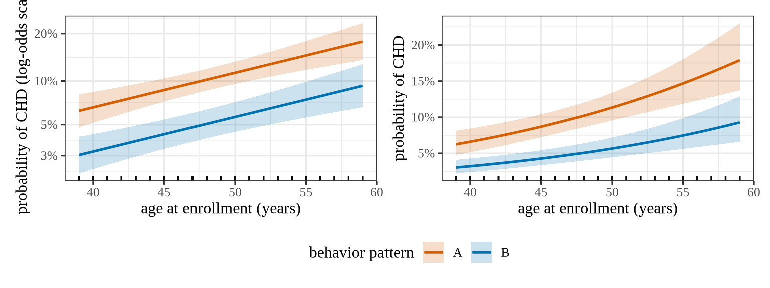
Example 2 (The age at enrollment curve on the logit and risk scales, for each behavior pattern) Plot the age at enrollment curve of Example 1, and turn it into a predicted probability of CHD. We draw one curve for each behavior pattern, type A and type B, from the one fitted model. The additive model is linear in its terms only on the logit scale, so there the s(age) curve is a partial effect. It adds to the others. The plotted log odds differ from s(age) only by a constant, the intercept plus the other terms at each curve’s covariate pattern. On the probability scale the effect of age depends on the other predictors, so each curve is drawn at a covariate pattern. That pattern fixes the other predictors. The coefficient of Example 1 for behavior pattern B shifts the whole curve, and both curves hold body mass index and systolic blood pressure fixed at their medians in the WCGS data. Both scales use predict() with type = "link", and the probability scale applies the inverse logit, plogis(), to the link-scale ends of the interval, so that the interval is built on the scale where the fit is approximately normal and stays inside (0, 1).
library(ggplot2)
library(patchwork)
# Two covariate patterns, one per behavior pattern:
# age varies,
# and the other predictors sit at typical values.
grid <- expand.grid(
age = seq(min(wcgs$age), max(wcgs$age), length.out = 100),
dibpat = levels(wcgs$dibpat)
)
grid$bmi <- median(wcgs$bmi)
grid$sbp <- median(wcgs$sbp)
grid$dibpat <- factor(grid$dibpat, levels = levels(wcgs$dibpat))
# Fit and standard error on the logit (link) scale,
# with the intercept and the other terms held at each pattern's values.
pred <- predict(m_wcgs, grid, type = "link", se.fit = TRUE)
link_scale <- data.frame(
age = grid$age, dibpat = grid$dibpat, fit = pred$fit,
lower = pred$fit - 2 * pred$se.fit, upper = pred$fit + 2 * pred$se.fit
)
# The inverse logit maps the fit and both interval ends to probabilities.
prob_scale <- within(link_scale, {
fit <- plogis(fit)
lower <- plogis(lower)
upper <- plogis(upper)
})
# Both panels share the bands, lines and rug.
# Only the y scale differs.
curve_panel <- function(df) {
ggplot(df, aes(age, fit, colour = dibpat, fill = dibpat)) +
geom_ribbon(aes(ymin = lower, ymax = upper), alpha = 0.2, colour = NA) +
geom_line(linewidth = 0.9) +
geom_rug(aes(x = age), data = wcgs, inherit.aes = FALSE, alpha = 0.05,
sides = "b") +
scale_colour_manual(values = c(A = "#D55E00", B = "#0072B2")) +
scale_fill_manual(values = c(A = "#D55E00", B = "#0072B2")) +
labs(x = "age at enrollment (years)", colour = "behavior pattern",
fill = "behavior pattern")
}
# The left panel is drawn on the log-odds scale,
# with its ticks put at the log odds of round probabilities,
# so that they read as risks.
risk_ticks <- c(0.03, 0.05, 0.1, 0.2)
p_link <- curve_panel(link_scale) +
scale_y_continuous(breaks = qlogis(risk_ticks),
labels = scales::label_percent()(risk_ticks)) +
labs(y = "probability of CHD (log-odds scale)")
p_prob <- curve_panel(prob_scale) +
scale_y_continuous(labels = scales::label_percent()) +
labs(y = "probability of CHD")
p_link + p_prob + plot_layout(guides = "collect")
# Predicted risks at two ages, for each behavior pattern.
pred_pts <- expand.grid(age = c(40, 55), dibpat = levels(wcgs$dibpat))
pred_pts$bmi <- median(wcgs$bmi)
pred_pts$sbp <- median(wcgs$sbp)
pred_pts$dibpat <- factor(pred_pts$dibpat, levels = levels(wcgs$dibpat))
pred_two <- predict(m_wcgs, pred_pts, type = "link", se.fit = TRUE)
risk_two <- plogis(pred_two$fit)
# The interval is built on the link scale, then mapped through the inverse logit.
risk_lower <- plogis(pred_two$fit - qnorm(0.975) * pred_two$se.fit)
risk_upper <- plogis(pred_two$fit + qnorm(0.975) * pred_two$se.fit)At the median body mass index and systolic blood pressure, the model gives a CHD probability of 6.6% (95% interval [5.2, 8.4]%) at age 40 for behavior pattern A and 14.7% ([11.9, 18.0]%) at age 55. For behavior pattern B the probabilities are 3.2% ([2.4, 4.3]%) at age 40 and 7.5% ([5.6, 9.8]%) at age 55. The type B curve lies below the type A curve at every age by the same amount on the logit scale, the type B coefficient, yet the gap on the probability scale grows with age, because the inverse logit steepens as the probability grows toward one half. The same logit-scale gap is a larger probability gap at a higher baseline risk.
Exercise 4 (Updating one component at a time)
Exercise 4 (Updating one component at a time) Suppose \(\beta_0\) and every component function except \(f_j\) are held fixed in the penalized criterion of Remark 2. What problem remains for \(f_j\)?
Solution 4. Define the partial residuals \(r_i = y_i - \beta_0 - \sum_{k \ne j} f_k(x_{ik})\). Only the terms involving \(f_j\) still vary, and they are \(\sum_i \paren{r_i - f_j(x_{ij})}^2 + \regpar_j \int \paren{f_j''(t)}^2\, dt\): a one-variable smoothing spline problem (Splines) for the response \(r\) against \(x_j\).
Exercise 5 (Updating one component at a time (part 2))
Exercise 5 (Updating one component at a time (part 2)) Use the setup of Exercise 4.
What is the solution to the problem that remains for \(f_j\)?
Solution 5. Its solution is \(\hat f_j = S_j\, \vec{r}\), where \(S_j\) is the smoother matrix of \(x_j\) with parameter \(\regpar_j\).
Theorem 1 (The backfitting update for one component)
Theorem 1 (The backfitting update for one component) Hold \(\beta_0\) and every component function except \(f_j\) fixed in the penalized criterion of Remark 2, and write \(r_i = y_i - \beta_0 - \sum_{k \ne j} f_k(x_{ik})\) for the partial residuals. The remaining problem is to minimize
\[\sum_i \paren{r_i - f_j(x_{ij})}^2 + \regpar_j \int \paren{f_j''(t)}^2\, dt\]
over \(f_j\). This is a one-variable smoothing spline problem for the response \(r\) against \(x_j\), and its solution is \(\hat f_j = S_j\, \vec{r}\), where \(S_j\) is the smoother matrix of \(x_j\) with parameter \(\regpar_j\).
Proof
Proof. By Solution 4 and Solution 5.
Example 3 (One backfitting step on the Auto data)
Example 3 (One backfitting step on the Auto data) In the Auto data [3], take mpg as the response with components in weight and horsepower. Start with \(\hat\beta_0 = \bar y\) and \(\hat f_{\text{weight}} = 0\), and update \(\hat f_{\text{horsepower}}\) by smoothing the partial residuals against horsepower:
import numpy as np
import pandas as pd
from scipy.interpolate import make_smoothing_spline
auto_bf = pd.read_csv("data/auto.csv").dropna(subset=["horsepower"])
auto_bf = auto_bf.groupby("horsepower", as_index=False).mean(numeric_only=True)
y_bf = auto_bf["mpg"].to_numpy(float)
# Partial residuals with beta_0 = mean(y) and the weight component still 0.
r_bf = y_bf - y_bf.mean()
f_hp = make_smoothing_spline(auto_bf["horsepower"].to_numpy(float), r_bf, lam=100.0)
print(np.round(f_hp(auto_bf["horsepower"].to_numpy(float))[:5], 2))[9.17 9.58 9.67 9.67 9.68]
[1] -6.14 -9.45 -8.33 -8.33 -7.34
The result is \(\hat f_{\text{horsepower}} = S_j \vec{r}\) of Theorem 1 for the one-variable smoothing spline.
Definition 4 (Backfitting)
Definition 4 (Backfitting) Backfitting fits an additive model by cycling through the components [8]. Start with \(\hat\beta_0 = \bar y\) and every \(\hat f_j = 0\), and repeat until the fits stop changing: for \(j = 1, \dots, p\),
Each step solves Theorem 1, so each step lowers the penalized criterion, and the cycle converges [1], [8].
Example 4 (An additive model for the Auto data)
Example 4 (An additive model for the Auto data) In the Auto data [3], predict mpg from horsepower, weight and year. Fit an additive model by backfitting, with the penalized natural spline smoother of Splines for each term: eight knots at quantiles of the predictor, and the same smoothing parameter \(\regpar = 0.1\) throughout, for standardized predictors. Compare it with a linear model by 5-fold cross-validation, using the same folds for both:
import numpy as np
import pandas as pd
from scipy import stats
auto_ad = pd.read_csv("data/auto.csv").dropna(subset=["horsepower"])
predictors_ad = ["horsepower", "weight", "year"]
X_ad = auto_ad[predictors_ad].to_numpy(float)
# Standardize each predictor, so one smoothing parameter suits all three.
X_ad = (X_ad - X_ad.mean(axis=0)) / X_ad.std(axis=0, ddof=1)
y_ad = auto_ad["mpg"].to_numpy(float)
def natural_basis(x, knots):
# 1, x, and N_{k+2} = d_k - d_{K-1}: natural cubic spline basis, as in the Splines chapter.
K = len(knots)
def d(k):
return (np.maximum(x - knots[k], 0) ** 3 - np.maximum(x - knots[-1], 0) ** 3) / (knots[-1] - knots[k])
return np.column_stack([np.ones_like(x), x] + [d(k) - d(K - 2) for k in range(K - 2)])
def natural_penalty(knots, grid_size=4000):
# Integral of N_j'' N_k'' by the trapezoid rule on a fine grid (N'' is piecewise linear).
K = len(knots)
t = np.linspace(knots[0], knots[-1], grid_size)
def d2(k):
return 6 * (np.maximum(t - knots[k], 0) - np.maximum(t - knots[-1], 0)) / (knots[-1] - knots[k])
second = np.column_stack([np.zeros_like(t)] * 2 + [d2(k) - d2(K - 2) for k in range(K - 2)])
w = np.full(grid_size, t[1] - t[0])
w[[0, -1]] /= 2
return second.T @ (second * w[:, None])
# Knots depend on the predictors only, never on mpg, so using all rows to place them
# does not leak the held-out responses. Ties in a predictor, such as year, can repeat a
# quantile, so keep each knot once.
knots_ad = [np.unique(np.quantile(X_ad[:, j], np.linspace(0, 1, 8))) for j in range(3)]
bases_ad = [natural_basis(X_ad[:, j], knots_ad[j]) for j in range(3)]
penalties_ad = [natural_penalty(k) for k in knots_ad]
lam_ad = 0.1
def backfit(bases, penalties, y, lam, n_iter=50):
n = len(y)
beta0 = y.mean()
# Each term's smoother maps partial residuals to spline coefficients.
maps = [np.linalg.solve(B.T @ B + lam * P, B.T) for B, P in zip(bases, penalties)]
fits = [np.zeros(n) for _ in bases]
coefs = [None] * len(bases)
centers = np.zeros(len(bases))
for _ in range(n_iter):
for j in range(len(bases)):
# Partial residuals: what the other terms leave unexplained.
partial = y - beta0 - sum(fits[k] for k in range(len(bases)) if k != j)
coefs[j] = maps[j] @ partial
fit = bases[j] @ coefs[j]
# Center each component, so the intercept stays the mean response.
centers[j] = fit.mean()
fits[j] = fit - centers[j]
return beta0, coefs, centers
def predict_additive(model, bases_new):
beta0, coefs, centers = model
return beta0 + sum(B @ c - m for B, c, m in zip(bases_new, coefs, centers))
fold_ad = np.arange(len(y_ad)) % 5
err_add, err_lin = [], []
for f in range(5):
train, test = fold_ad != f, fold_ad == f
model = backfit([B[train] for B in bases_ad], penalties_ad, y_ad[train], lam_ad)
err_add.append(y_ad[test] - predict_additive(model, [B[test] for B in bases_ad]))
design = np.column_stack([np.ones(len(y_ad)), X_ad])
coef_lin = np.linalg.lstsq(design[train], y_ad[train], rcond=None)[0]
err_lin.append(y_ad[test] - design[test] @ coef_lin)
print(round(np.sqrt(np.mean(np.concatenate(err_lin) ** 2)), 3),
round(np.sqrt(np.mean(np.concatenate(err_add) ** 2)), 3))3.427 2.825
def mean_ci_py(sq):
# A 95% t interval for a mean, here of squared cross-validated errors.
half = stats.t.ppf(0.975, df=len(sq) - 1) * sq.std(ddof=1) / np.sqrt(len(sq))
return sq.mean() - half, sq.mean() + half
sq_lin = np.concatenate(err_lin) ** 2
sq_add = np.concatenate(err_add) ** 2
# RMSE intervals are the square roots of the mean-squared-error intervals;
# the paired difference is taken car by car, as both models score the same cars.
print(np.round(np.sqrt(mean_ci_py(sq_lin)), 3), np.round(np.sqrt(mean_ci_py(sq_add)), 3))[3.088 3.735] [2.532 3.091]
[2.33 5.19]
auto_ad <- na.omit(read.csv("data/auto.csv")[, c("mpg", "horsepower", "weight", "year")])
predictors_ad <- c("horsepower", "weight", "year")
# Standardize each predictor, so one smoothing parameter suits all three.
X_ad <- scale(as.matrix(auto_ad[, predictors_ad]))
y_ad <- auto_ad$mpg
natural_basis <- function(x, knots) {
# 1, x, and N_{k+2} = d_k - d_{K-1}: natural cubic spline basis, as in the Splines chapter.
K <- length(knots)
d <- function(k) {
(pmax(x - knots[k], 0)^3 - pmax(x - knots[K], 0)^3) / (knots[K] - knots[k])
}
cbind(1, x, sapply(1:(K - 2), function(k) d(k) - d(K - 1)))
}
natural_penalty <- function(knots, grid_size = 4000) {
# Integral of N_j'' N_k'' by the trapezoid rule on a fine grid (N'' is piecewise linear).
K <- length(knots)
t <- seq(knots[1], knots[K], length.out = grid_size)
d2 <- function(k) {
6 * (pmax(t - knots[k], 0) - pmax(t - knots[K], 0)) / (knots[K] - knots[k])
}
second <- cbind(0, 0, sapply(1:(K - 2), function(k) d2(k) - d2(K - 1)))
w <- rep(t[2] - t[1], grid_size)
w[c(1, grid_size)] <- w[1] / 2
crossprod(second, second * w)
}
# Knots depend on the predictors only, never on mpg, so using all rows to place them
# does not leak the held-out responses. Ties in a predictor, such as year, can repeat a
# quantile, so keep each knot once.
knots_ad <- lapply(1:3, function(j) unique(quantile(X_ad[, j], seq(0, 1, length.out = 8))))
bases_ad <- lapply(1:3, function(j) natural_basis(X_ad[, j], knots_ad[[j]]))
penalties_ad <- lapply(knots_ad, natural_penalty)
lam_ad <- 0.1
backfit <- function(bases, penalties, y, lambda, n_iter = 50) {
n <- length(y)
beta0 <- mean(y)
# Each term's smoother maps partial residuals to spline coefficients.
maps <- Map(function(B, P) solve(crossprod(B) + lambda * P, t(B)), bases, penalties)
fits <- replicate(length(bases), numeric(n), simplify = FALSE)
coefs <- vector("list", length(bases))
centers <- numeric(length(bases))
for (iter in seq_len(n_iter)) {
for (j in seq_along(bases)) {
# Partial residuals: what the other terms leave unexplained.
partial <- y - beta0 - Reduce(`+`, fits[-j], numeric(n))
coefs[[j]] <- drop(maps[[j]] %*% partial)
fit <- drop(bases[[j]] %*% coefs[[j]])
# Center each component, so the intercept stays the mean response.
centers[j] <- mean(fit)
fits[[j]] <- fit - centers[j]
}
}
list(beta0 = beta0, coefs = coefs, centers = centers)
}
predict_additive <- function(model, bases_new) {
parts <- Map(function(B, cf, ctr) drop(B %*% cf) - ctr,
bases_new, model$coefs, model$centers)
model$beta0 + Reduce(`+`, parts)
}
fold_ad <- (seq_along(y_ad) - 1) %% 5
err_add <- err_lin <- numeric(0)
design_ad <- cbind(1, X_ad)
for (f in 0:4) {
train <- fold_ad != f
test <- fold_ad == f
model <- backfit(lapply(bases_ad, function(B) B[train, ]), penalties_ad,
y_ad[train], lam_ad)
err_add <- c(err_add, y_ad[test] - predict_additive(
model, lapply(bases_ad, function(B) B[test, ])))
coef_lin <- qr.solve(design_ad[train, ], y_ad[train])
err_lin <- c(err_lin, y_ad[test] - design_ad[test, ] %*% coef_lin)
}
round(c(linear = sqrt(mean(err_lin^2)), additive = sqrt(mean(err_add^2))), 3) linear additive
3.427 2.825
# A 95% t interval for a mean, here of squared cross-validated errors.
mean_ci <- function(sq) {
half <- qt(0.975, df = length(sq) - 1) * sd(sq) / sqrt(length(sq))
c(lower = mean(sq) - half, upper = mean(sq) + half)
}
# The intervals are for the mean squared error; square-root them to get RMSE.
ci_lin <- sqrt(mean_ci(err_lin^2))
ci_add <- sqrt(mean_ci(err_add^2))
# Both models predict the same cars, so the paired differences are taken car by car.
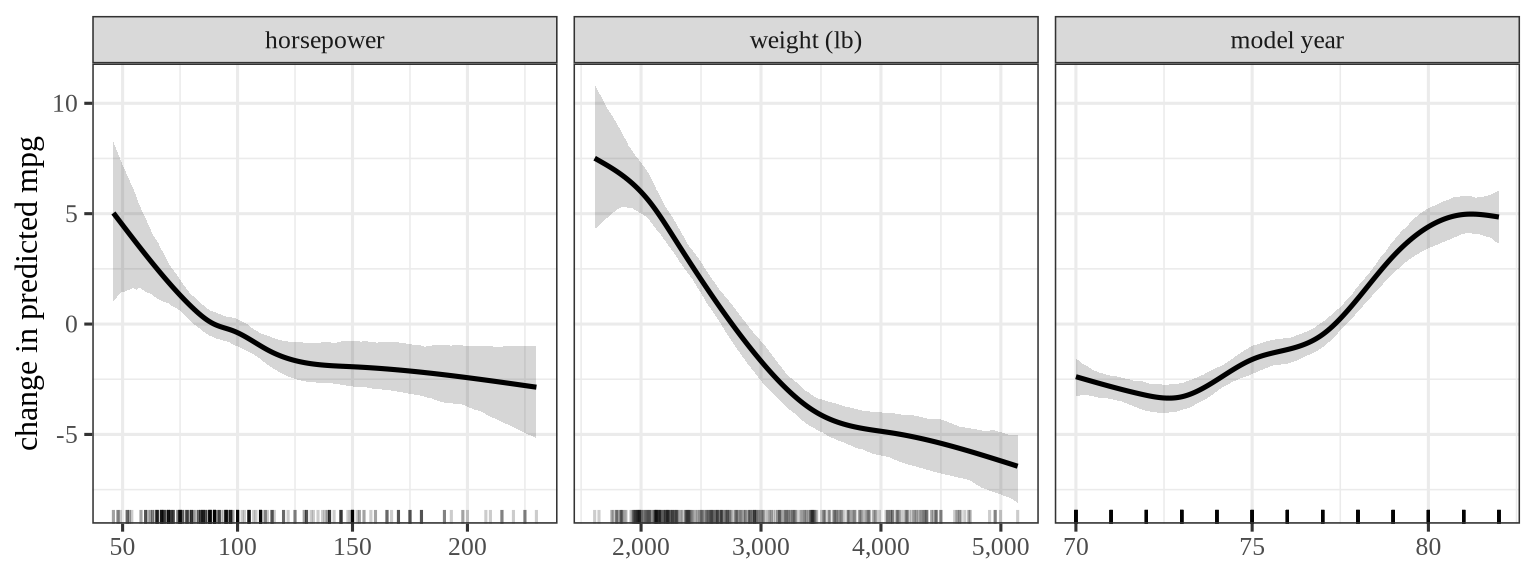
diff_ad <- mean_ci(err_lin^2 - err_add^2)The cross-validated sRMSE is 3.43 mpg for the linear model (95% interval [3.09, 3.74]) and 2.83 mpg for the additive model ([2.53, 3.09]): letting each predictor have its own smooth shape cuts the error by 18 percent. Each interval is a \(t\) interval for the mean of the 392 squared cross-validated errors, with its endpoints square-rooted. Comparing the two intervals ignores that both models are scored on the same cars, so the comparison is better made car by car: the linear model’s sMSE is larger by 3.8 mpg\(^2\) on average, with a 95% interval of [2.3, 5.2], which excludes 0. These intervals are approximate: the five training sets overlap, so the errors are not independent and the intervals tend to be too narrow [9]. They reflect which cars were scored, not which cars were in a training set. The smoothing parameter \(\regpar = 0.1\) was fixed in advance; choosing it, term by term, by cross-validation as in Splines is the usual next step.
library(ggplot2)
model_full <- backfit(bases_ad, penalties_ad, y_ad, lam_ad)
grids_ad <- lapply(1:3, function(j) {
seq(min(X_ad[, j]), max(X_ad[, j]), length.out = 200)
})
# The centered component functions of a fitted model, stacked over the three grids.
component_curves <- function(model) {
unlist(lapply(1:3, function(j) {
drop(natural_basis(grids_ad[[j]], knots_ad[[j]]) %*% model$coefs[[j]]) -
model$centers[j]
}))
}
# A bootstrap band: refit the model on cars drawn with replacement, and take the
# middle 95% of the refitted curves at each grid point.
set.seed(1)
boot_curves <- replicate(200, {
rows <- sample(nrow(X_ad), replace = TRUE)
component_curves(backfit(
lapply(bases_ad, function(B) B[rows, ]), penalties_ad, y_ad[rows], lam_ad
))
})
band_ad <- t(apply(boot_curves, 1, quantile, c(0.025, 0.975)))
# The model works on standardized predictors; the plot shows each one in its
# original units (horsepower, pounds, model year).
ad_center <- attr(X_ad, "scaled:center")
ad_scale <- attr(X_ad, "scaled:scale")
term_labels <- c(horsepower = "horsepower", weight = "weight (lb)",
year = "model year")
to_original <- function(z, j) z * ad_scale[j] + ad_center[j]
effects_ad <- data.frame(
x = unlist(lapply(1:3, function(j) to_original(grids_ad[[j]], j))),
effect = component_curves(model_full),
lower = band_ad[, 1],
upper = band_ad[, 2],
term = factor(rep(predictors_ad, each = 200), levels = predictors_ad,
labels = term_labels[predictors_ad])
)
rug_ad <- data.frame(
x = unlist(lapply(1:3, function(j) to_original(X_ad[, j], j))),
term = factor(rep(predictors_ad, each = nrow(X_ad)), levels = predictors_ad,
labels = term_labels[predictors_ad])
)
ggplot(effects_ad, aes(x, effect)) +
geom_ribbon(aes(ymin = lower, ymax = upper), alpha = 0.2) +
geom_line(linewidth = 0.9) +
geom_rug(aes(x = x), data = rug_ad, inherit.aes = FALSE, alpha = 0.2,
sides = "b") +
facet_wrap(~term, scales = "free_x") +
# Whole-number ticks, so that model years read 70, 75, 80.
scale_x_continuous(
breaks = function(lims) {
ticks <- scales::extended_breaks()(lims)
ticks[ticks == round(ticks)]
},
labels = scales::label_comma()
) +
labs(x = NULL, y = "change in predicted mpg")Each curve shows how the prediction changes with one predictor while the others are held at their averages, and is read like a coefficient in a linear model, except that its slope varies. The additive form has one limit: it cannot represent an effect of one predictor that depends on another. A two-variable smooth term, or a product feature, restores an interaction, but the model then loses the simple one-curve-per-predictor picture.
In practice, software chooses the smoothing parameters automatically and handles non-Gaussian responses: the mgcv package in R [2], and the pygam and statsmodels packages in Python.