Simulation Studies

Last modified: 2026-11-07 21:34:29 (PST)

Theory often cannot give the bias, variance or coverage of an estimator when the estimator or the data distribution is complicated. A simulation study measures the same properties for any estimator a computer can run. It generates many data sets from a distribution whose parameters are known, applies the estimator to each, and summarizes the results.

This page defines the parts of a simulation study, shows how to measure the study’s own accuracy, and works one example in R and Python whose answer is known.

1 The data-generating process

Definition 1 (Data-generating process) The data-generating process (DGP) of a simulation is the joint probability distribution \(F_{\theta_0}\) from which it draws its data \(X_1, \ldots, X_n\), with the number of observations \(n\) and the parameter value \(\theta_0\) fixed and known:

\[X_1, \ldots, X_n \sim F_{\theta_0}.\]

Example 1 (A normal data-generating process)  

Let \(X_1, \ldots, X_n\) be IID normal random variables with expectation \(\mu= 0\) and variance \(\sigma^2= 4\), with \(n = 10\). The distribution of these variables is a data-generating process, and the estimand \(\sigma^2= 4\) is known exactly, so the error of any estimator of \(\sigma^2\) can be computed.

2 Replications and simulation studies

Definition 2 (Replication) A replication of a simulation is one run of its steps: draw a data set \(X_1, \ldots, X_n^{(m)}\) from the data-generating process, then compute the estimate \(T_m \stackrel{\text{def}}{=}\hat{\theta}\mathopen{}\left(X_1, \ldots, X_n^{(m)}\right)\mathclose{}\), where \(\hat{\theta}\) is an estimator, for \(m = 1, \ldots, M\). Different replications draw their data sets independently.

Example 2 (A replication of the normal data-generating process)  

For the normal data-generating process, one replication draws \(n = 10\) values from the normal distribution with expectation \(0\) and variance \(4\). It then computes the estimate \(T_m\) of the variance \(\sigma^2\) from those 10 values. A second replication draws 10 new values, independently of the first, and computes \(T_{m + 1}\).

Definition 3 (Simulation study) A simulation study runs \(M\) replications of one data-generating process and one estimator, then summarizes the estimates \(T_1, \ldots, T_M\) to learn the estimator’s sampling distribution.

Example 3 (A simulation study of a variance estimator)  

For the normal data-generating process, a simulation study of one estimator of the variance \(\sigma^2\) runs \(M\) replications of that process and that estimator. The \(M\) estimates \(T_1, \ldots, T_M\) then show how the estimator behaves across repeated data sets.

3 Simulation estimates

Definition 4 (Simulation estimate) A simulation estimate of the expectation \({\mathbb{E}\mathopen{}\left[T\right]\mathclose{}}\) of an estimate \(T\) is the average of the replications’ estimates \(T_1, \ldots, T_M\):

\[{{\bar{T}}_{M}} \stackrel{\text{def}}{=}\frac{1}{M}\sum_{m=1}^{M} T_m.\]

Example 4 (A simulation estimate from three replications)  

Suppose \(M = 3\) replications give the estimates \(T_1 = 3\), \(T_2 = 5\) and \(T_3 = 4\). Then the simulation estimate of \({\mathbb{E}\mathopen{}\left[T\right]\mathclose{}}\) is

\[{{\bar{T}}_{3}} = \frac{3 + 5 + 4}{3} = 4.\]

Definition 5 (Simulation estimate of the bias) Let \(\theta\) be an estimand, let \(\hat{\theta}\) be an estimator, and let \(T_1, \ldots, T_M\) be its estimates from \(M\) replications. The simulation estimate of the bias of \(\hat{\theta}\) is the simulation estimate \({{\bar{T}}_{M}}\) of \({\mathbb{E}\mathopen{}\left[\hat{\theta}\right]\mathclose{}}\), minus \(\theta\):

\[{{\bar{T}}_{M}} - \theta.\]

Example 5 (A simulation estimate of the bias from three replications)  

Continue the three replications, and let the estimand be \(\theta= 5\). Then the simulation estimate of the bias is

\[{{\bar{T}}_{3}} - \theta= 4 - 5 = -1.\]

Definition 6 (Simulation estimate of the mean squared error) Let \(\theta\) be an estimand, let \(\hat{\theta}\) be an estimator, and let \(T_1, \ldots, T_M\) be its estimates from \(M\) replications. The simulation estimate of the mean squared error of \(\hat{\theta}\) is the average of the squared differences \(\mathopen{}\left(T_m - \theta\right)\mathclose{}^2\):

\[\frac{1}{M}\sum_{m=1}^{M} \mathopen{}\left(T_m - \theta\right)\mathclose{}^2.\]

Example 6 (A simulation estimate of the mean squared error from three replications)  

Continue the three replications with \(\theta= 5\). The squared differences are \(\mathopen{}\left(3 - 5\right)\mathclose{}^2= 4\), \(\mathopen{}\left(5 - 5\right)\mathclose{}^2= 0\) and \(\mathopen{}\left(4 - 5\right)\mathclose{}^2= 1\), so the simulation estimate of the mean squared error is

\[\frac{4 + 0 + 1}{3} = \frac{5}{3}.\]

Remark 1 (Simulation estimates in Bayesian inference). The Monte Carlo estimate of a posterior expectation is the same average, taken over draws from a posterior distribution instead of over replications of a data-generating process.

4 Monte Carlo error

Definition 7 (Monte Carlo standard error) The Monte Carlo standard error (MCSE) of a simulation estimate \({{\bar{T}}_{M}}\) is its standard error over repeated simulation studies:

\[{\operatorname{SE}\mathopen{}\left({{\bar{T}}_{M}}\right)\mathclose{}} = {\operatorname{SD}\mathopen{}\left({{\bar{T}}_{M}}\right)\mathclose{}}.\]

Theorem 1 (Monte Carlo standard error of a simulation estimate) Let \(T_1, \ldots, T_M\) be the estimates of \(M\) replications of a simulation study, which are IID with expectation \({\mathbb{E}\mathopen{}\left[T\right]\mathclose{}}\) and finite variance \({\operatorname{Var}\mathopen{}\left(T\right)\mathclose{}}\). Then the simulation estimate \({{\bar{T}}_{M}}\) is unbiased for \({\mathbb{E}\mathopen{}\left[T\right]\mathclose{}}\), and its Monte Carlo standard error is

\[{\operatorname{SE}\mathopen{}\left({{\bar{T}}_{M}}\right)\mathclose{}} = \frac{{\operatorname{SD}\mathopen{}\left(T\right)\mathclose{}}}{\sqrt{M}}.\]

Proof. By the mean and variance of a sum of IID random variables, the sum \(S_M \stackrel{\text{def}}{=}\sum_{m=1}^{M} T_m\) has \({\mathbb{E}\mathopen{}\left[S_M\right]\mathclose{}} = M\,{\mathbb{E}\mathopen{}\left[T\right]\mathclose{}}\) and \({\operatorname{Var}\mathopen{}\left(S_M\right)\mathclose{}} = M\,{\operatorname{Var}\mathopen{}\left(T\right)\mathclose{}}\). Since \({{\bar{T}}_{M}} = S_M / M\):

\[ \begin{aligned} {\mathbb{E}\mathopen{}\left[{{\bar{T}}_{M}}\right]\mathclose{}} &= \frac{{\mathbb{E}\mathopen{}\left[S_M\right]\mathclose{}}}{M} && \text{(constants factor out of expectations)}\\ &= \frac{M\,{\mathbb{E}\mathopen{}\left[T\right]\mathclose{}}}{M} && \text{(substitute ${\mathbb{E}\mathopen{}\left[S_M\right]\mathclose{}}$)}\\ &= \frac{M}{M}\,{\mathbb{E}\mathopen{}\left[T\right]\mathclose{}} && \text{(regroup the factors)}\\ &= 1 \cdot {\mathbb{E}\mathopen{}\left[T\right]\mathclose{}} && \text{($M / M = 1$)}\\ &= {\mathbb{E}\mathopen{}\left[T\right]\mathclose{}} && \text{(multiplying by 1 changes nothing)} \end{aligned} \]

For the variance:

\[ \begin{aligned} {\operatorname{Var}\mathopen{}\left({{\bar{T}}_{M}}\right)\mathclose{}} &= \frac{{\operatorname{Var}\mathopen{}\left(S_M\right)\mathclose{}}}{M^2} && \text{(a constant factor $c$ scales variance by $c^2$)}\\ &= \frac{M\,{\operatorname{Var}\mathopen{}\left(T\right)\mathclose{}}}{M^2} && \text{(substitute ${\operatorname{Var}\mathopen{}\left(S_M\right)\mathclose{}}$)}\\ &= \frac{M\,{\operatorname{Var}\mathopen{}\left(T\right)\mathclose{}}}{M \cdot M} && \text{(write $M^2$ as $M \cdot M$)}\\ &= \frac{M}{M} \cdot \frac{{\operatorname{Var}\mathopen{}\left(T\right)\mathclose{}}}{M} && \text{(split the fraction into two factors)}\\ &= 1 \cdot \frac{{\operatorname{Var}\mathopen{}\left(T\right)\mathclose{}}}{M} && \text{($M / M = 1$)}\\ &= \frac{{\operatorname{Var}\mathopen{}\left(T\right)\mathclose{}}}{M} && \text{(multiplying by 1 changes nothing)}\\ {\operatorname{SE}\mathopen{}\left({{\bar{T}}_{M}}\right)\mathclose{}} &= \sqrt{{\operatorname{Var}\mathopen{}\left({{\bar{T}}_{M}}\right)\mathclose{}}} && \text{(standard error is the standard deviation)}\\ &= \sqrt{\frac{{\operatorname{Var}\mathopen{}\left(T\right)\mathclose{}}}{M}} && \text{(substitute ${\operatorname{Var}\mathopen{}\left({{\bar{T}}_{M}}\right)\mathclose{}}$)}\\ &= \frac{\sqrt{{\operatorname{Var}\mathopen{}\left(T\right)\mathclose{}}}}{\sqrt{M}} && \text{(the square root of a quotient is the quotient of square roots)}\\ &= \frac{{\operatorname{SD}\mathopen{}\left(T\right)\mathclose{}}}{\sqrt{M}} && \text{(the standard deviation is the square root of the variance)} \end{aligned} \]

Remark 2 (Reporting a Monte Carlo standard error). The standard deviation \({\operatorname{SD}\mathopen{}\left(T\right)\mathclose{}}\) in Theorem 1 is unknown, so a study reports the sample standard deviation \(s_T\) of the estimates \(T_1, \ldots, T_M\) divided by \(\sqrt{M}\) in its place. That Monte Carlo standard error shrinks like \(1 / \sqrt{M}\), so quadrupling the number of replications halves it. A simulation estimate should be reported with its Monte Carlo standard error, so a reader can tell a real difference from random variation in the simulation.

5 Seeds

Definition 8 (Seed) A seed is the integer that sets the starting state of a computer’s pseudorandom number generator, so that rerunning a simulation with the same seed reproduces the same random draws:

\[\text{seed} \mapsto U_1, U_2, \ldots\]

Remark 3 (Setting seeds). Set the seed once, at the top of the simulation, and record its value with the results. Different software uses different generators, so the same seed gives different draws in R and in Python. Both give correct simulation estimates, which agree up to their Monte Carlo standard errors.

6 A worked simulation study

Example 7 (Simulating the bias of the divide-by-\(n\) variance estimator) For the data-generating process with \(\mu= 0\), \(\sigma^2= 4\) and \(n = 10\), we simulate the bias of the divide-by-\(n\) estimator \(\hat{\sigma}^2\) of \(\sigma^2\) from the example of a biased variance estimator. That example shows that the bias is exactly \(-\sigma^2/ n = -0.4\), so the simulation can be checked against the known answer.

Each replication draws \(n = 10\) values and computes one estimate of \(\sigma^2\). We run \(M = 10000\) replications, set the seed once at the start, and report the simulation estimate of the bias with its Monte Carlo standard error. The choice \(M = 10000\) gives a Monte Carlo standard error of about \(0.02\), small next to the bias.

n <- 10
sigma_sq <- 4
n_reps <- 10000
n_draws <- n_reps * n
sigma <- sqrt(sigma_sq)

set.seed(571)
draws <- rnorm(n_draws, mean = 0, sd = sigma)
# Each row is one replication's data set.
x <- matrix(draws, nrow = n_reps)

x_bar <- rowMeans(x)
deviations <- x - x_bar
squared_deviations <- deviations^2
var_hat <- rowMeans(squared_deviations)

bias_hat <- mean(var_hat) - sigma_sq
mc_se <- sd(var_hat) / sqrt(n_reps)

c(
  simulation_estimate = bias_hat,
  mc_standard_error = mc_se,
  known_bias = -sigma_sq / n
)
#> simulation_estimate   mc_standard_error          known_bias 
#>          -0.3915413           0.0169017          -0.4000000
import numpy as np

n = 10
sigma_sq = 4
n_reps = 10000

rng = np.random.default_rng(571)
# Each row is one replication's data set.
x = rng.normal(loc=0, scale=np.sqrt(sigma_sq), size=(n_reps, n))

x_bar = x.mean(axis=1, keepdims=True)
var_hat = ((x - x_bar) ** 2).mean(axis=1)

bias_hat = var_hat.mean() - sigma_sq
mc_se = var_hat.std(ddof=1) / np.sqrt(n_reps)

print(f"simulation estimate: {bias_hat:.3f}")
#> simulation estimate: -0.390
print(f"mc standard error:   {mc_se:.3f}")
#> mc standard error:   0.017
print(f"known bias:          {-sigma_sq / n:.3f}")
#> known bias:          -0.400

The R simulation estimate of the bias is -0.392, with a Monte Carlo standard error of 0.017. It is within 0.5 Monte Carlo standard errors of the known bias -0.4. The Python run uses a different random number generator, so its estimate differs slightly, but it too agrees with -0.4 up to its Monte Carlo standard error.

Figure 1 shows the sampling distribution of \(\hat{\sigma}^2\) that the replications trace out. Its histogram uses 40 equal-width bins, which put about 250 of the 10^{4} estimates in the average bin. Fewer bins, such as 10, would hide the right skew of the distribution in a few wide bars. More bins, such as 200, would leave about 50 estimates per bin on average, and random bar-to-bar variation would hide the shape. The bin count changes only the picture, not any number reported above.

[Code]
estimates <- tibble::tibble(var_hat = var_hat)
mean_var_hat <- mean(var_hat)
line_values <- c(sigma_sq, mean_var_hat)
line_labels <- c("True variance", "Average estimate")
means <- tibble::tibble(value = line_values, line = line_labels)

estimates |>
  ggplot() +
  aes(x = var_hat) +
  # check-unexplained-choices: allow
  geom_histogram(bins = 40, fill = "grey80", color = "grey40") +
  geom_vline(
    data = means,
    mapping = aes(xintercept = value, linetype = line)
  ) +
  labs(x = "Estimate of the variance", y = "Replications", linetype = NULL)
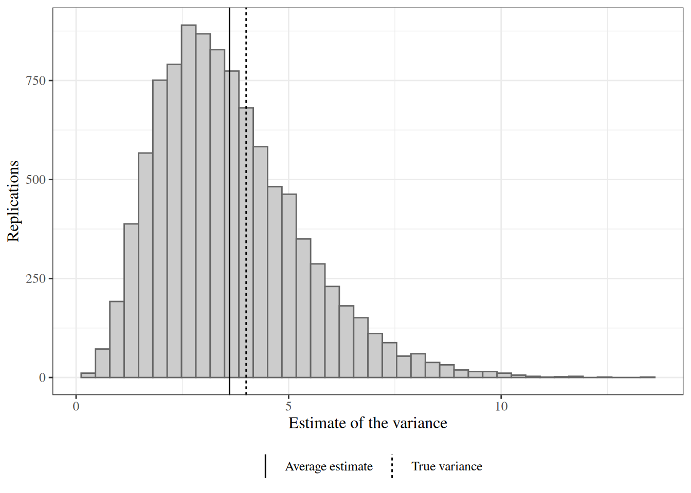
Figure 1: Estimates of the variance from 10,000 replications. The vertical lines mark the true variance 4 and the average estimate, which falls below it by the bias.
A histogram of 10,000 divide-by-n variance estimates, right-skewed, with one vertical line at the true variance 4 and a second, slightly to its left, at the average estimate.

The distribution is right-skewed, and its average sits below the true variance, which is the bias.

References