Exploratory Data Analysis
Last modified: 2026-11-07 21:34:29 (PST)
1 Introduction
Before fitting a model, it is good practice to explore and summarize the data. Exploratory data analysis (EDA) serves several purposes:
- understanding the distribution of each variable individually;
- detecting unusual values, outliers, and missing data;
- identifying patterns and relationships among variables;
- motivating choices of model structure, such as transformations;
- providing context for interpreting model results.
1.1 The WCGS data
This page illustrates exploratory data analysis using data from the Western Collaborative Group Study (WCGS) [2]. Vittinghoff et al. [1, p. 9] describe the study this way:
The Western Collaborative Group Study (WCGS) was a large epidemiological study designed to investigate the association between the “type A” behavior pattern and coronary heart disease (CHD).
Exercise 1 (Type A behavior) What is “type A” behavior?
Solution 1. From Wikipedia’s article “Type A and Type B personality theory”:
The hypothesis describes Type A individuals as outgoing, ambitious, rigidly organized, highly status-conscious, impatient, anxious, proactive, and concerned with time management….
The hypothesis describes Type B individuals as a contrast to those of Type A. Type B personalities, by definition, are noted to live at lower stress levels. They typically work steadily and may enjoy achievement, although they have a greater tendency to disregard physical or mental stress when they do not achieve.
1.2 Study design
The WCGS began in 1960 with 3,524 male volunteers employed by 11 California companies. Participants were 39 to 59 years old and free of heart disease, as determined by electrocardiogram. After the initial screening, various exclusions reduced the study population to 3,154 men and the number of companies to 10. The cohort comprised both blue- and white-collar employees. Average follow-up was 8.5 years, with repeat examinations.
At baseline, the study collected:
- socio-demographic characteristics: age, education, marital status, income, and occupation;
- physical and physiological measurements: height, weight, blood pressure, electrocardiogram, and corneal arcus;
- biochemical measurements: cholesterol and lipoprotein fractions;
- medical and family history, and use of medications;
- behavioral data: the Type A interview, smoking, exercise, and alcohol use.
Later surveys added anthropometry, triglycerides, the Jenkins Activity Survey, and caffeine use.
1.3 Loading the data
The WCGS data are distributed with Vittinghoff et al. [1] on the book’s companion website, as a Stata file that R can read directly:
The rmb R package includes the same file, which these notes use so that rendering does not depend on the website. haven::as_factor() converts the Stata value labels to factors:
[Code]
# attach a descriptive label to each variable;
# gtsummary tables print these labels instead of the column names:
wcgs_labels <- c(
  age = "Age (years)",
  chol = "Cholesterol (mg/dL)",
  sbp = "Systolic BP (mmHg)",
  dbp = "Diastolic BP (mmHg)",
  bmi = "BMI (kg/m^2)",
  weight = "Weight (lbs)",
  ncigs = "Cigarettes per day",
  chd69 = "CHD event by 1969",
  smoke = "Current smoker",
  arcus = "Arcus senilis",
  dibpat = "Behavioral pattern (A/B)",
  behpat = "Behavioral pattern (A1/A2/B3/B4)",
  wghtcat = "Weight category",
  agec = "Age group"
)
for (var in names(wcgs_labels)) {
  attr(wcgs[[var]], "label") <- wcgs_labels[[var]]
}

wcgs_labels
#>                                age                               chol
#>                      "Age (years)"              "Cholesterol (mg/dL)"
#>                                sbp                                dbp
#>               "Systolic BP (mmHg)"              "Diastolic BP (mmHg)"
#>                                bmi                             weight
#>                     "BMI (kg/m^2)"                     "Weight (lbs)"
#>                              ncigs                              chd69
#>               "Cigarettes per day"                "CHD event by 1969"
#>                              smoke                              arcus
#>                   "Current smoker"                    "Arcus senilis"
#>                             dibpat                             behpat
#>         "Behavioral pattern (A/B)" "Behavioral pattern (A1/A2/B3/B4)"
#>                            wghtcat                               agec
#>                  "Weight category"                        "Age group"
The dataset has one row per participant:
dplyr::glimpse(wcgs)
#> Rows: 3,154
#> Columns: 22
#> $ age      <dbl> 50, 51, 59, 51, 44, 47, 40, 41, 50, 43, 59, 54, 48, 39, 49, 5…
#> $ arcus    <dbl> 1, 0, 1, 1, 0, 0, 0, 0, 1, 0, 0, 0, 0, 0, 0, 1, 0, 0, 0, 0, 1…
#> $ behpat   <fct> A1, A1, A1, A1, A1, A1, A1, A1, A1, A1, A1, A1, A1, A1, A1, A…
#> $ bmi      <dbl> 31.3210, 25.3286, 28.6939, 22.1487, 22.3130, 27.1177, 23.2420…
#> $ chd69    <fct> No, No, No, No, No, No, No, No, No, No, No, No, No, Yes, No, …
#> $ chol     <dbl> 249, 194, 258, 173, 214, 206, 190, 212, 130, 233, 181, 214, 2…
#> $ dbp      <dbl> 90, 74, 94, 80, 80, 76, 78, 84, 70, 80, 86, 76, 78, 74, 80, 7…
#> $ dibpat   <fct> Type A, Type A, Type A, Type A, Type A, Type A, Type A, Type …
#> $ height   <dbl> 67, 73, 70, 69, 71, 64, 70, 70, 71, 68, 72, 67, 71, 70, 73, 7…
#> $ id       <dbl> 2343, 3656, 3526, 22057, 12927, 16029, 3894, 11389, 12681, 10…
#> $ lnsbp    <dbl> 4.88280, 4.78749, 5.06259, 4.83628, 4.83628, 4.75359, 4.80402…
#> $ lnwght   <dbl> 5.29832, 5.25750, 5.29832, 5.01064, 5.07517, 5.06259, 5.08760…
#> $ ncigs    <dbl> 25, 25, 0, 0, 0, 80, 0, 25, 0, 25, 10, 0, 20, 0, 4, 0, 0, 20,…
#> $ sbp      <dbl> 132, 120, 158, 126, 126, 116, 122, 130, 112, 120, 130, 118, 1…
#> $ smoke    <fct> Yes, Yes, No, No, No, Yes, No, Yes, No, Yes, Yes, No, Yes, No…
#> $ t1       <dbl> -1.633353, -4.063366, 0.639729, 1.121768, 2.425011, -0.787520…
#> $ time169  <dbl> 1367, 2991, 2960, 3069, 3081, 2114, 2929, 3010, 3104, 2861, 2…
#> $ typchd69 <dbl> 0, 0, 0, 0, 0, 0, 0, 0, 0, 0, 0, 0, 0, 1, 0, 0, 0, 0, 0, 0, 0…
#> $ uni      <dbl> 0.4860738, 0.1859543, 0.7277991, 0.6244636, 0.3789776, 0.7355…
#> $ weight   <dbl> 200, 192, 200, 150, 160, 158, 162, 160, 195, 187, 206, 152, 1…
#> $ wghtcat  <fct> 170-200, 170-200, 170-200, 140-170, 140-170, 140-170, 140-170…
#> $ agec     <fct> 46-50, 51-55, 56-60, 51-55, 41-45, 46-50, 35-40, 41-45, 46-50…
1.4 Populations and samples
Definition 1 (Population) A population is the entire collection of units (people, animals, objects, or events) that a study aims to learn about.
Source: Wikipedia contributors [3].
Definition 2 (Population distribution) The population distribution of a variable \(X\) is the distribution of \(X\) for a unit chosen at random from a population (Definition 1): the probability that \(X\) falls in a set \(A\) is
\[{\mathbb{P}\mathopen{}\left(A\right)\mathclose{}} \stackrel{\text{def}}{=}\Pr(X \in A),\]
where the probability refers to the random choice of the unit.
Definition 3 (Observation) An observation is the set of values recorded for the variables on one unit of a population (Definition 1). Each recorded value is a realization of the corresponding variable.
Example 1 (One observation in the WCGS) Each row of the wcgs data frame is one observation: the values recorded for one participant. The first participant’s observation has age 50 years and cholesterol 249 mg/dL.
Definition 4 (Sample) A sample of size \(n\) is the data \(x_1, \ldots, x_n\) observed on \(n\) units drawn from a population (Definition 1).
Definition 5 (Random sample) A sample (Definition 4) is a random sample when the units are chosen by a chance mechanism such that the observations are independent and identically distributed draws from the population distribution (Definition 2):
\[X_1, \ldots, X_n \operatorname{iid}\ \mathbb{P},\]
where \(\mathbb{P}\) is the population distribution.
Source: Wikipedia contributors [4].
Example 2 (Population and sample in the WCGS) In 1960, the WCGS recruited employed men aged 39 to 59 years in California. Take that group of men as the study’s population (Definition 1), so the population distribution (Definition 2) of cholesterol is its distribution among those men. The wcgs data frame is the sample (Definition 4): it holds 3154 of the men in that population. The men volunteered, through 10 companies, so the sample is not a random sample (Definition 5) of the population. Its sample mean cholesterol, 226.4 mg/dL, describes these 3154 men exactly, but it estimates the population mean well only to the extent that the volunteers resemble the rest of the population.
Definition 6 (Population parameter) A population parameter is a number computed from the population distribution (Definition 2), such as its population mean.
Example 3 (A population parameter in the WCGS) In Example 2, the population mean of cholesterol is a population parameter. It describes all the men in the study’s population (Definition 1). We know only the mean cholesterol of the sample (Definition 4) of the wcgs data, 226.4 mg/dL.
2 Summarizing a single variable
2.1 Measures of center
Definition 7 (Sample mean) The sample mean of \(n\) observations \(x_1, \ldots, x_n\) is:
\[{\bar{x}}\stackrel{\text{def}}{=}\frac{1}{n}\sum_{i=1}^nx_i\]
Example 5 (Sample mean versus population mean of cholesterol) The population mean of cholesterol is the expectation of the population distribution (Definition 2). It is a fixed number that we do not know. The sample mean (Definition 7) of the wcgs data, 226.4 mg/dL, is computed from the observed data. A different sample from the same population would give a different sample mean, while the population mean would not change.
Definition 8 (Sample median) The sample median is the middle value when the observations are sorted in increasing order. In terms of the order statistics \(x_{(1)} \le \cdots \le x_{(n)}\):
- if \(n\) is odd, the median is \(x_{((n+1)/2)}\);
- if \(n\) is even, the median is \(\frac{1}{2}\mathopen{}\left(x_{(n/2)} + x_{(n/2 + 1)}\right)\mathclose{}\).
Source: Wikipedia contributors [5].
Example 6 (Median cholesterol in the WCGS)
The median cholesterol is a little lower than the sample mean (Example 4). Cholesterol has a longer right tail than left tail (the maximum is 645 mg/dL), and the large values in that tail pull the sample mean upward but barely change which value is in the middle. A median is less sensitive to extreme values than a sample mean.
2.2 Measures of spread
Definition 9 (Sample variance) The sample variance of \(n \ge 2\) observations is:
\[s^2 \stackrel{\text{def}}{=}\frac{1}{n-1} \sum_{i=1}^n(x_i- {\bar{x}})^2\]
Source: Wikipedia contributors [6].
Definition 10 (Sample standard deviation) The sample standard deviation is the square root of the sample variance:
\[s \stackrel{\text{def}}{=}\sqrt{s^2}\]
Source: Wikipedia contributors [7].
Remark 2 (Units of the standard deviation). The standard deviation has the same units as the observations, which makes it easier to interpret than the variance, whose units are squared.
Definition 11 (Quartiles (first quartile, third quartile, 25th percentile, 75th percentile)) The quartiles are the first quartile \(Q_1\) and the third quartile \(Q_3\), the sample 0.25 and 0.75 quantiles (sample quantile). The first quartile is also called the 25th percentile, and the third quartile is also called the 75th percentile.
Source: Wikipedia contributors [8].
Remark 3 (Quartiles in software). With an odd number of observations, the sample 0.5 quantile equals the sample median; with an even number they can differ, because the median averages the two middle order statistics. Software packages compute quartiles with different quantile definitions, so they can disagree slightly for the same data (quantile conventions); R’s quantile(type = 1) matches this definition, and R’s default, type = 7, interpolates.
Example 8 (Quartiles and IQR of cholesterol in the WCGS)
The middle half of the cholesterol values span 56 mg/dL. Like the median, the IQR does not depend on the most extreme values, so it is less sensitive to outliers than the standard deviation.
2.3 Summary statistics in R
The summary() function reports the minimum, quartiles, mean, maximum, and number of missing values in one call; its quartiles use R’s default interpolating quantile rule (type = 7), so they can differ slightly from Definition 11:
For a formatted table of several variables at once, gtsummary::tbl_summary() is useful (Table 1).
| Characteristic | N = 3,1541 |
|---|---|
| Age (years) | 46.3 (5.5); 45.0 [42.0, 50.0] |
| Cholesterol (mg/dL) | 226.4 (43.4); 223.0 [197.0, 253.0] |
| Unknown | 12 |
| Systolic BP (mmHg) | 128.6 (15.1); 126.0 [120.0, 136.0] |
| Diastolic BP (mmHg) | 82.0 (9.7); 80.0 [76.0, 86.0] |
| BMI (kg/m^2) | 24.5 (2.6); 24.4 [23.0, 25.8] |
| Weight (lbs) | 170.0 (21.1); 170.0 [155.0, 182.0] |
| 1 Mean (SD); Median [Q1, Q3] | |
2.4 Binary and categorical variables
Definition 13 (Sample proportion) For a binary variable with values coded 1 (“success”) and 0, the sample proportion of successes is:
\[\hat{p} \stackrel{\text{def}}{=}\frac{k}{n}\]
where \(k\) is the number of successes and \(n\) is the number of observations.
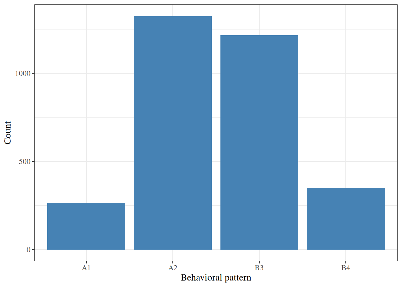
For categorical variables with more than two levels, the natural descriptive statistics are the count of observations in each category and the corresponding proportions (Table 2).
| Characteristic | N = 3,1541 |
|---|---|
| CHD event by 1969 | 257 (8.1%) |
| Current smoker | 1,502 (48%) |
| Behavioral pattern (A/B) | |
| Type B | 1,565 (50%) |
| Type A | 1,589 (50%) |
| Behavioral pattern (A1/A2/B3/B4) | |
| A1 | 264 (8.4%) |
| A2 | 1,325 (42%) |
| B3 | 1,216 (39%) |
| B4 | 349 (11%) |
| Weight category | |
| < 140 | 232 (7.4%) |
| 140-170 | 1,538 (49%) |
| 170-200 | 1,171 (37%) |
| > 200 | 213 (6.8%) |
| 1 n (%) | |
- Hogg et al. [10, Sec. 6.1], pp. 233–244 covers descriptive statistics.
- Rice [11, Secs. 10.4–10.5], pp. 392–401 covers measures of location and dispersion.
3 Graphical methods
Graphs can reveal features of a distribution that summary statistics miss, such as skewness, multiple peaks, and outliers. Different types of graph suit different types of variable.
3.1 Histograms
Definition 14 (Histogram) A histogram displays the distribution of a continuous variable by dividing the variable’s range into intervals and drawing a bar over each interval whose height is the number (or proportion) of observations in that interval.
Source: Wikipedia contributors [12].
Definition 15 (Bin) A bin of a histogram is one of its intervals.
[Code]
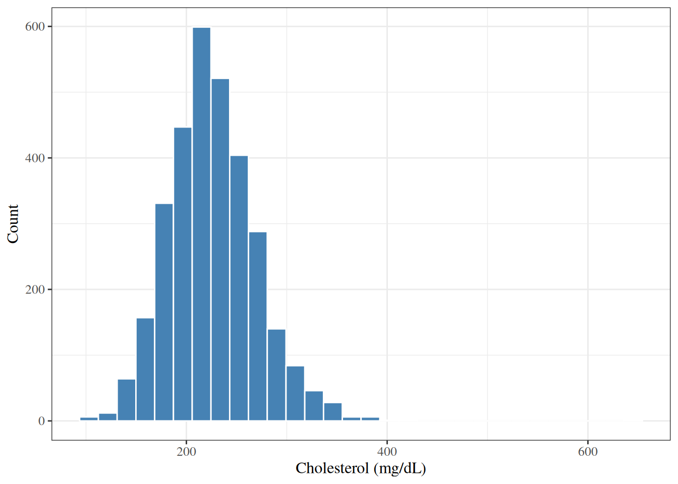
Figure 1 shows a single-peaked distribution with a longer right tail than left tail: 97% of the values lie between 150 and 350 mg/dL, but the largest value is 645 mg/dL.
3.2 Density plots
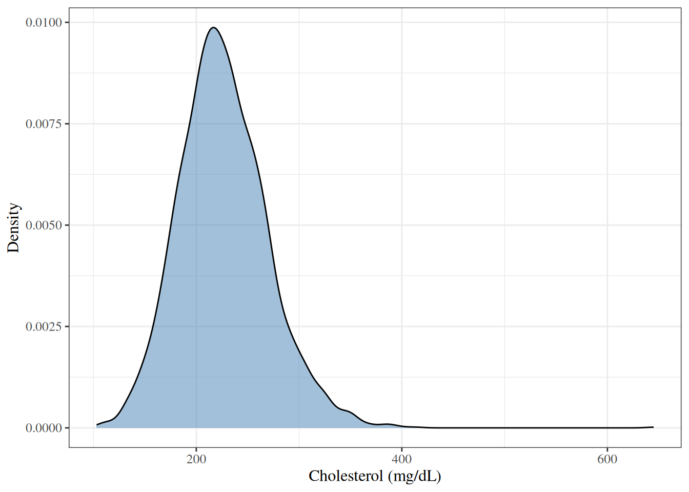
Definition 16 (Density plot) A density plot draws a smooth curve that estimates the probability density of a continuous variable, scaled so that the area under the curve is 1.
Source: Wikipedia contributors [13].
[Code]
3.3 Box plots
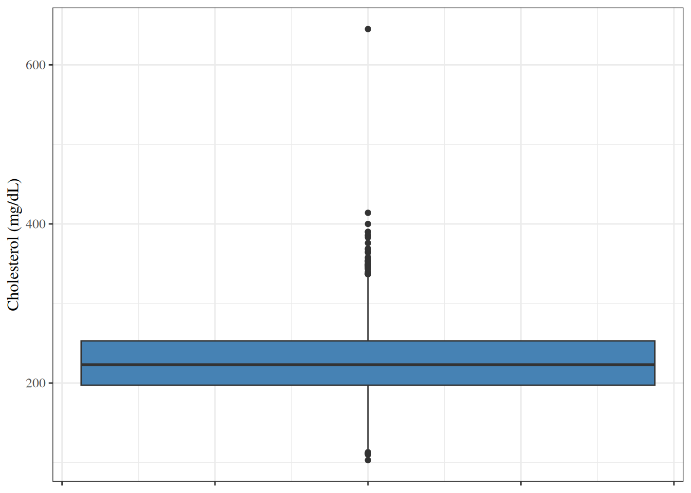
Definition 17 (Box plot (box-and-whisker plot)) A box plot (or box-and-whisker plot) summarizes the distribution of a continuous variable:
- the box spans the first to the third quartile, so its length is the IQR;
- a line inside the box marks the median;
- the whiskers extend from the box to the most extreme observations within \(1.5 \times \text{IQR}\) of the box;
- observations beyond the whiskers are plotted individually, as potential outliers.
Source: Wikipedia contributors [14].
Remark 4 (Whisker rules). The \(1.5 \times \text{IQR}\) whisker rule is the default in R’s boxplot() and ggplot2::geom_boxplot(); other software and authors use other rules, such as whiskers that run to the minimum and maximum.
[Code]
3.4 Bar charts
Definition 18 (Bar chart) A bar chart displays the number or proportion of observations in each category of a categorical variable, as one bar per category.
Source: Wikipedia contributors [15].
[Code]
3.5 Normal quantile-quantile plots
Definition 19 (Normal quantile-quantile plot) A normal quantile-quantile (Q-Q) plot plots the sorted observations (order statistics) against the corresponding quantiles of a standard Gaussian distribution. If the variable is approximately Gaussian, the points fall close to a straight line.
Source: Wikipedia contributors [16].
[Code]
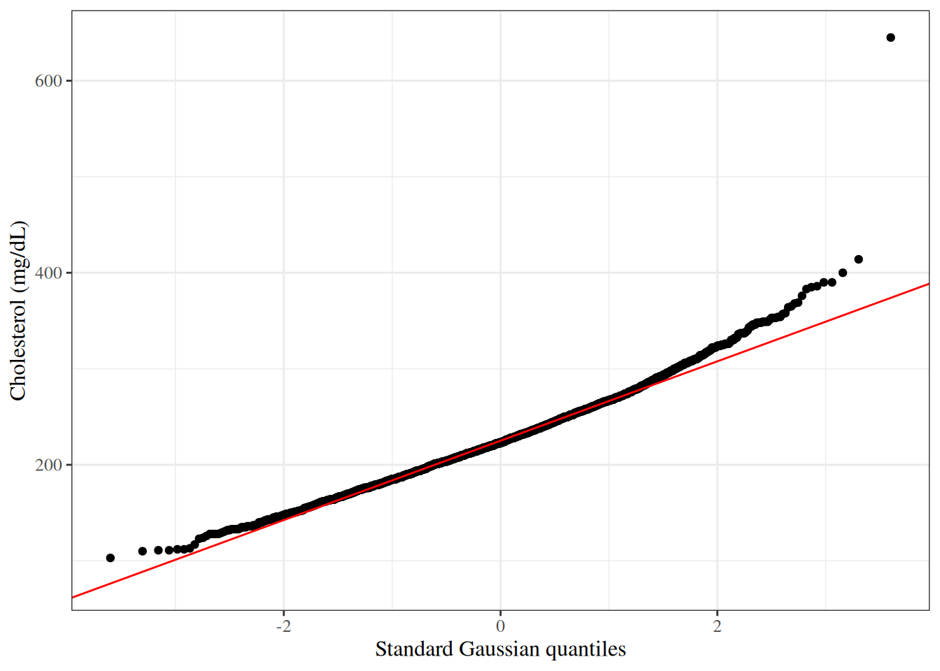
In Figure 5, the points curve above the reference line at the right, which matches the long right tail in Figure 1.
- Hogg et al. [10, Sec. 6.2], pp. 245–255 covers exploratory data analysis.
- Rice [11, Sec. 10.2.3], pp. 385–388 covers quantile-quantile plots.
- Rice [11, Sec. 10.3], pp. 389–391 covers histograms, density curves and stem-and-leaf plots.
- Rice [11, Sec. 10.6], pp. 402–403 covers boxplots.
4 Bivariate relationships
4.1 Two continuous variables
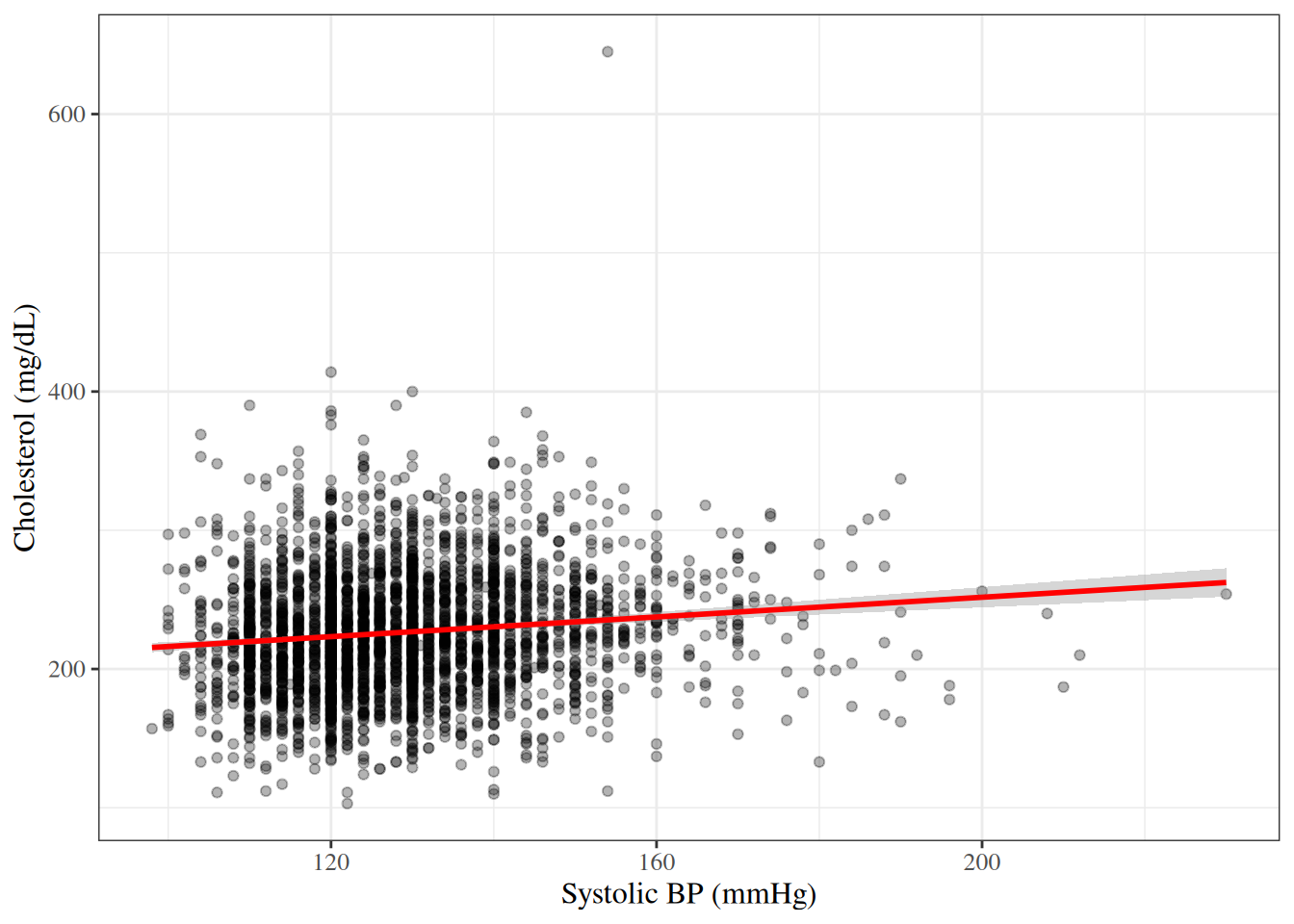
Definition 20 (Scatter plot) A scatter plot displays the joint distribution of two continuous variables by plotting each observation as a point, with one variable on each axis.
Source: Wikipedia contributors [17].
[Code]
Definition 21 (Pearson correlation coefficient) The Pearson correlation coefficient of \(n\) paired observations \((x_1, y_1), \ldots, (x_n, y_n)\) is:
\[r \stackrel{\text{def}}{=}\frac{\sum_{i=1}^n(x_i- {\bar{x}})(y_i- {\bar{y}})} {\sqrt{\sum_{i=1}^n(x_i- {\bar{x}})^2} \sqrt{\sum_{i=1}^n(y_i- {\bar{y}})^2}}\]
It is defined when neither variable is constant, so that both sums of squares are positive.
Source: Wikipedia contributors [18].
Remark 5 (The Pearson correlation coefficient estimates the population correlation). The Pearson correlation coefficient is a sample estimate of the population correlation.
Theorem 1 (Range of the correlation coefficient) The Pearson correlation coefficient satisfies \(-1 \le r \le 1\). Moreover, \(r = 1\) if and only if the points \((x_i, y_i)\) lie on a straight line with positive slope, and \(r = -1\) if and only if they lie on a straight line with negative slope.
Proof. Write \(a_i \stackrel{\text{def}}{=}x_i- \bar x\) and \(b_i \stackrel{\text{def}}{=}y_i- \bar y\), so that \(r = \sum_i a_i b_i / \mathopen{}\left(\sqrt{\sum_i a_i^2} \sqrt{\sum_i b_i^2}\right)\mathclose{}\). The Cauchy–Schwarz inequality states that \(\mathopen{}\left|\sum_i a_i b_i\right|\mathclose{} \le \sqrt{\sum_i a_i^2} \sqrt{\sum_i b_i^2}\), with equality if and only if one of the vectors \((a_1, \ldots, a_n)\) and \((b_1, \ldots, b_n)\) is a scalar multiple of the other. Dividing both sides by the (positive) right-hand side gives \(\mathopen{}\left|r\right|\mathclose{} \le 1\).
Equality \(\mathopen{}\left|r\right|\mathclose{} = 1\) therefore holds if and only if \(b_i = c \, a_i\) for some constant \(c \ne 0\) and every \(i\), that is, \(y_i= \bar y + c(x_i- \bar x)\): the points lie on a line with slope \(c\). Then \(\sum_i a_i b_i = c \sum_i a_i^2\) has the sign of \(c\), so \(r = 1\) when \(c > 0\) and \(r = -1\) when \(c < 0\).
Example 10 (Correlation between cholesterol and blood pressure in the WCGS)
The correlation is positive but small: cholesterol tends to be slightly higher in participants with higher systolic blood pressure, consistent with the shallow slope and wide scatter in Figure 6.
Correlation measures linear association only
Two variables can be strongly related and still have a correlation near zero, if the relationship is not linear. For example, if \(y_i= x_i^2\), the \(x_i\) are symmetric around 0, and the \(\mathopen{}\left|x_i\right|\mathclose{}\) are not all equal, then \(r = 0\), although \(y\) is a function of \(x\). Correlation also does not imply causation.
Rice [11, Sec. 10.7], pp. 404–406 covers scatterplots.
4.2 A continuous variable by a categorical variable
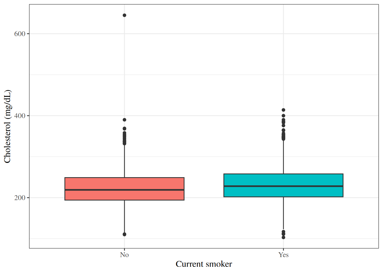
Side-by-side box plots compare the distribution of a continuous variable across the groups defined by a categorical variable (Figure 7 and Figure 8).
[Code]
[Code]
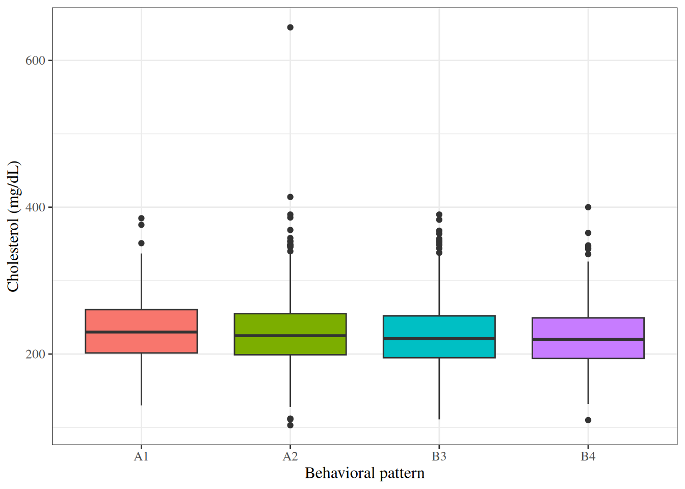
Table 3 computes summary statistics separately for each group.
[Code]
| Characteristic |
Overall N = 3,1541 |
No N = 2,8971 |
Yes N = 2571 |
|---|---|---|---|
| Cholesterol (mg/dL) | 226.4 (43.4) | 224.3 (42.2) | 250.1 (49.4) |
| Unknown | 12 | 12 | 0 |
| Systolic BP (mmHg) | 128.6 (15.1) | 128.0 (14.7) | 135.4 (17.5) |
| BMI (kg/m^2) | 24.5 (2.6) | 24.5 (2.6) | 25.1 (2.6) |
| 1 Mean (SD) | |||
4.3 Two categorical variables
Definition 22 (Contingency table (cross-tabulation)) A contingency table (or cross-tabulation) displays the joint frequencies of two categorical variables: each cell counts the observations with one combination of categories. For two binary variables, the contingency table is a \(2 \times 2\) table with cells \(a\), \(b\), \(c\), and \(d\):
| Outcome = 1 | Outcome = 0 | Total | |
|---|---|---|---|
| Exposure = 1 | \(a\) | \(b\) | \(a + b\) |
| Exposure = 0 | \(c\) | \(d\) | \(c + d\) |
| Total | \(a + c\) | \(b + d\) | \(n\) |
Source: Wikipedia contributors [19].
Example 11 (Smoking and CHD in the WCGS)
Row proportions give the distribution of CHD status within each smoking group:
Table 4 shows the same counts as a formatted table.
[Code]
| Characteristic |
Overall N = 3,1541 |
No N = 2,8971 |
Yes N = 2571 |
|---|---|---|---|
| Current smoker | 1,502 (48%) | 1,343 (46%) | 159 (62%) |
| 1 n (%) | |||
5 Data transformations
When a continuous variable has a right-skewed distribution (a longer tail to the right than to the left), a logarithmic transformation often makes the distribution more symmetric. A log-transformed variable also has a multiplicative interpretation: an increase of 1 in \(\log(x)\) corresponds to multiplying \(x\) by \(e \approx 2.72\), because \(\log(x) + 1 = \log(e \cdot x)\).
The WCGS dataset already contains log-transformed versions of two variables:
-
lnsbp: \(\log(\text{SBP})\); -
lnwght: \(\log(\text{weight})\).
lnsbp.
[Code]
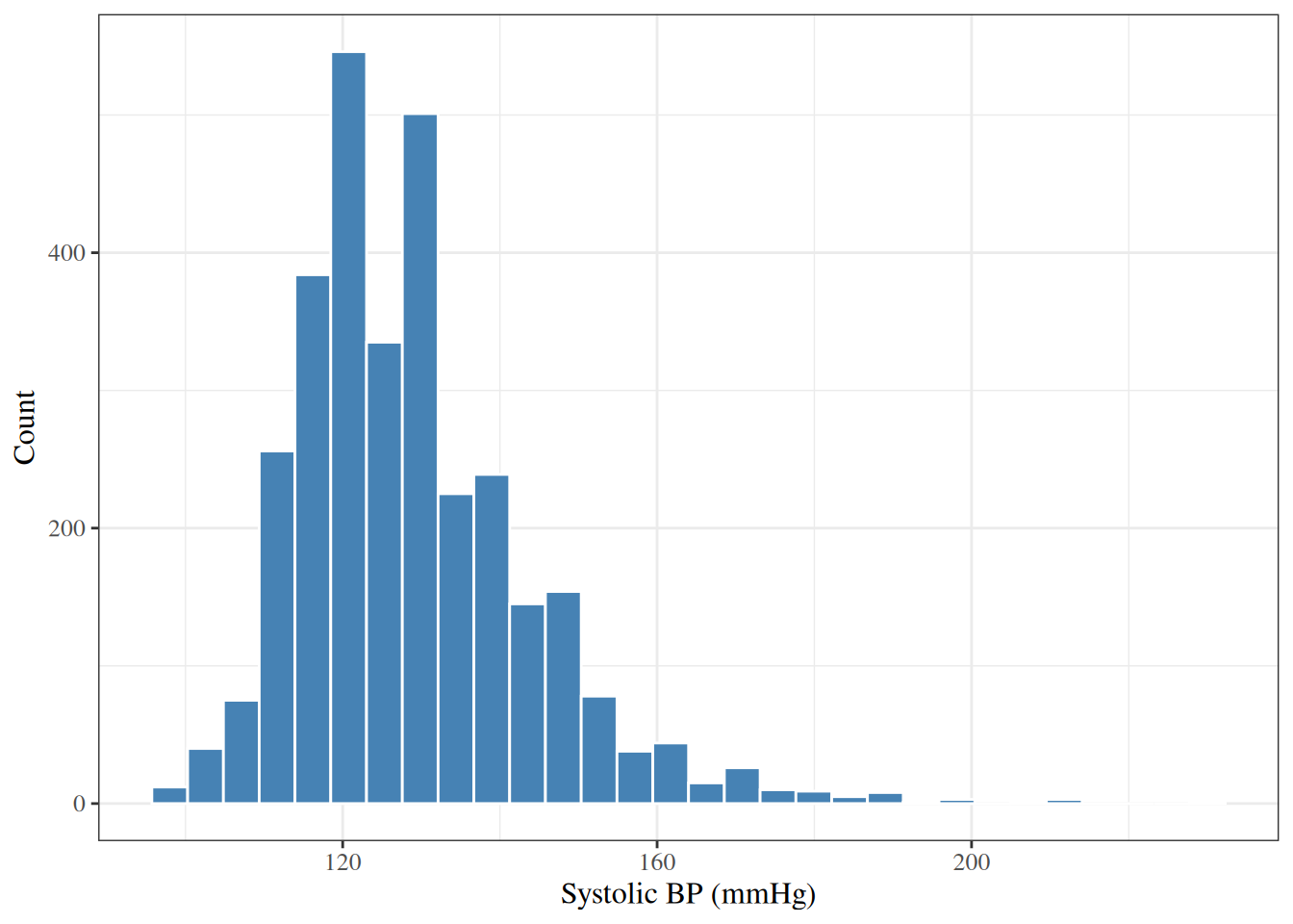
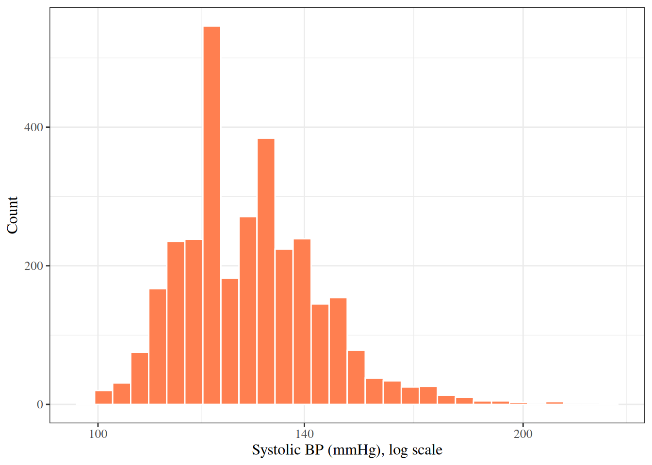
The log-transformed SBP is less skewed than the raw SBP (sample skewness 0.74 versus 1.2), but still not symmetric. Whether to transform a variable in a regression model depends on the assumptions of that model and on the scientific question.
5.1 Rescaling a variable
Exercise 2 (A standardized cholesterol value) In the WCGS data, cholesterol (chol) is measured in mg/dL.
- Compute the sample mean and sample standard deviation of
chol. - A man has
cholequal to 250 mg/dL. By how many standard deviations does his value differ from the sample mean, and in which direction? - What are the units of your answer to part 2?
Solution 2.
The sample mean is 226.4 mg/dL and the sample standard deviation is 43.4 mg/dL.
\((250 - \bar x) / s\) is 0.54: his cholesterol is 0.54 standard deviations above the sample mean.
The numerator is in mg/dL and the denominator is in mg/dL, so the answer has no units.
Definition 23 (Standardization (z-scoring, standard scaling)) Let \(x_1, \ldots, x_n\) be \(n \ge 2\) observations of a variable with sample mean \(\bar x\) and sample standard deviation \(s > 0\). The standardized value of \(x_i\) is
\[z_i \stackrel{\text{def}}{=}\frac{x_i- \bar x}{s}\]
Standardization is also called z-scoring or standard scaling.
Source: Wikipedia contributors [20].
Remark 6 (Source: Standardization). James et al. [21, Sec. 4.7.6], p. 183. Géron [22, Ch. 2] describes the same operation but says it divides by the variance; the standard deviation is used here, as in James et al. [21].
Remark 7 (Standardized values have no units). In Exercise 2, the standardized value of a cholesterol of 250 mg/dL is the number of sample standard deviations between 250 and the sample mean. Standardizing puts variables measured in different units on a comparable scale. For example, a salary in dollars and an age in years both become unitless numbers of standard deviations.
Theorem 2 (Standardized values have sample mean 0 and sample standard deviation 1) For \(n \ge 2\) observations with \(s > 0\), the standardized values \(z_1, \ldots, z_n\) have sample mean \(0\) and sample standard deviation \(1\).
Proof. The sample mean of the \(z_i\) is \[ \begin{aligned} \frac{1}{n}\sum_{i=1}^n\frac{x_i- \bar x}{s} &= \frac{1}{s} \mathopen{}\left(\frac{1}{n}\sum_{i=1}^nx_i- \bar x\right)\mathclose{}\\ &= \frac{1}{s} (\bar x - \bar x)\\ &= 0. \end{aligned} \] Since the sample mean of the \(z_i\) is \(0\), their sample variance is \[ \begin{aligned} \frac{1}{n-1} \sum_{i=1}^nz_i^2 &= \frac{1}{s^2} \cdot \frac{1}{n-1} \sum_{i=1}^n(x_i- \bar x)^2\\ &= \frac{s^2}{s^2}\\ &= 1, \end{aligned} \] so their sample standard deviation is \(\sqrt{1} = 1\).
Remark 8 (Source: Standardized values have sample mean 0 and sample standard deviation 1). Stated for the standardized Caravan variables in James et al. [21, Sec. 4.7.6], p. 183; the proof is the elementary calculation.
Example 12 (Standardizing cholesterol in R) In R, scale() returns the standardized values of a column, as a one-column matrix. For the WCGS cholesterol values:
The sample mean is \(0\) up to rounding error, and the sample standard deviation is \(1\), as Theorem 2 says. The na.rm = TRUE is needed because 12 of the cholesterol values are missing.
Definition 24 (Min-max scaling) Let \(x_1, \ldots, x_n\) be observations of a variable with minimum \(x_{\min}\) and maximum \(x_{\max} > x_{\min}\). The min-max scaled value of \(x_i\) is
\[\frac{x_i- x_{\min}}{x_{\max} - x_{\min}}\]
Source: Géron [22, Ch. 2]; Wikipedia contributors [23].
Remark 9 (Min-max scaling and outliers). Every min-max scaled value lies in \([0, 1]\): the minimum maps to \(0\) and the maximum maps to \(1\). For example, if median incomes range from 0 to 15, an income of 0 maps to \(0\), and an income of 15 maps to \(1\).
Min-max scaling is sensitive to outliers. For example, suppose one income of 100 is recorded by mistake. The maximum is then 100, so min-max scaling maps all the other incomes into \([0, 0.15]\). Standardization changes them much less [22, Ch. 2], “Feature Scaling”.
Example 13 (Min-max scaling of cholesterol in the WCGS)
The smallest cholesterol value maps to 0 and the largest maps to 1. The scaled values keep the shape of the distribution but have no units.
6 An exploratory data analysis workflow
A typical exploratory data analysis proceeds as follows:
- Understand the dataset: the number of observations and variables, and each variable’s type.
-
Examine each variable individually:
- continuous: histogram, box plot, mean, SD, median, IQR;
- categorical: bar chart, frequency table;
- note missing values, unusual values, and outliers.
-
Examine relationships between variables:
- two continuous variables: scatter plot, correlation;
- continuous by categorical: side-by-side box plots, group means;
- two categorical variables: contingency table.
- Consider transformations for skewed continuous variables.
- Summarize the findings to guide model-building decisions.
Table 5 summarizes selected WCGS variables in one table.
[Code]
| Characteristic | N = 3,1541 |
|---|---|
| Age (years) | 45.0 (42.0, 50.0) |
| Cholesterol (mg/dL) | 223 (197, 253) |
| Unknown | 12 |
| Systolic BP (mmHg) | 126 (120, 136) |
| Diastolic BP (mmHg) | 80 (76, 86) |
| BMI (kg/m^2) | 24.39 (22.96, 25.84) |
| Weight (lbs) | 170 (155, 182) |
| Cigarettes per day | 0 (0, 20) |
| CHD event by 1969 | 257 (8.1%) |
| Current smoker | 1,502 (48%) |
| Behavioral pattern (A/B) | |
| Type B | 1,565 (50%) |
| Type A | 1,589 (50%) |
| Behavioral pattern (A1/A2/B3/B4) | |
| A1 | 264 (8.4%) |
| A2 | 1,325 (42%) |
| B3 | 1,216 (39%) |
| B4 | 349 (11%) |
| 1 Median (Q1, Q3); n (%) | |
7 Further reading
Plotting a Binary Outcome shows how to plot a 0/1 outcome against a continuous feature, where scatterplot dots would pile into two stripes. It draws a rug and two histograms of the WCGS data, in R and Python.