Newton’s Method

Last modified: 2026-11-13 13:00:00 (PST)

Source

This section is adapted from the Newton-Raphson and gradient descent parts of Zhou [1], used under the MIT License (see the license text in Linear Algebra). The source motivates the Newton step informally, as the step that minimizes a quadratic approximation; here Theorem 1 proves that the step is that approximation’s exact minimizer. In the source’s zigzag example the starting value of the objective is \(\tfrac{1}{2}(b^2 + b)\), not \(\tfrac{1}{2}(1 + b^2)\) as the source writes; the ratio of successive values is unaffected. In the same example the source’s formula for \(\mathord{\smash[b]{\underset{\raise.3ex\hbox{$\scriptstyle\sim$}}{x}}\vphantom{x}}^{(1)}\) has \(\mathord{\smash[b]{\underset{\raise.3ex\hbox{$\scriptstyle\sim$}}{x}}\vphantom{x}}^{(1)}\) on its right side where \(\mathord{\smash[b]{\underset{\raise.3ex\hbox{$\scriptstyle\sim$}}{x}}\vphantom{x}}^{(0)}\) is meant. These parts of the source are not part of this section:

• the quadratic convergence theorem for Newton’s method in general, and its remedies for instability (a positive definite substitute for the Hessian, and shortening the Newton step by a search along its direction)
• its remark that Hessians are expensive to compute
• the convergence-rate theorem for strongly convex functions
• gradient descent with momentum, and its optimal parameters
• Nesterov acceleration, and stochastic gradient descent
• its code and animations

1 Iterative methods

Definition 1 (Iterative method) An iterative method [2] starts from a point \(\mathord{\smash[b]{\underset{\raise.3ex\hbox{$\scriptstyle\sim$}}{x}}\vphantom{x}}^{(0)}\) and computes \(\mathord{\smash[b]{\underset{\raise.3ex\hbox{$\scriptstyle\sim$}}{x}}\vphantom{x}}^{(t+1)}\) from \(\mathord{\smash[b]{\underset{\raise.3ex\hbox{$\scriptstyle\sim$}}{x}}\vphantom{x}}^{(t)}\) by a fixed rule, for \(t = 0, 1, 2, \ldots\).

Definition 2 (Iterate) In an iterative method (Definition 1), the points \(\mathord{\smash[b]{\underset{\raise.3ex\hbox{$\scriptstyle\sim$}}{x}}\vphantom{x}}^{(t)}\) are its iterates.

Definition 3 (Error of an iterate) For a point \(\mathord{\smash[b]{\underset{\raise.3ex\hbox{$\scriptstyle\sim$}}{x}}\vphantom{x}}^*\) that an iterative method (Definition 1) is meant to reach, \(\mathopen{}\left\lVert\mathord{\smash[b]{\underset{\raise.3ex\hbox{$\scriptstyle\sim$}}{x}}\vphantom{x}}^{(t)} - \mathord{\smash[b]{\underset{\raise.3ex\hbox{$\scriptstyle\sim$}}{x}}\vphantom{x}}^*\right\rVert\mathclose{}\) is the error of the iterate \(\mathord{\smash[b]{\underset{\raise.3ex\hbox{$\scriptstyle\sim$}}{x}}\vphantom{x}}^{(t)}\) (Definition 2).

Definition 4 (Convergence of a sequence of vectors) A sequence \(\mathord{\smash[b]{\underset{\raise.3ex\hbox{$\scriptstyle\sim$}}{x}}\vphantom{x}}^{(0)}, \mathord{\smash[b]{\underset{\raise.3ex\hbox{$\scriptstyle\sim$}}{x}}\vphantom{x}}^{(1)}, \ldots\) in \(\mathbb{R}^p\) converges to \(\mathord{\smash[b]{\underset{\raise.3ex\hbox{$\scriptstyle\sim$}}{x}}\vphantom{x}}^* \in \mathbb{R}^p\) if the sequence of distances \(\mathopen{}\left\lVert\mathord{\smash[b]{\underset{\raise.3ex\hbox{$\scriptstyle\sim$}}{x}}\vphantom{x}}^{(t)} - \mathord{\smash[b]{\underset{\raise.3ex\hbox{$\scriptstyle\sim$}}{x}}\vphantom{x}}^*\right\rVert\mathclose{}\) converges to \(0\). For \(p = 1\), \(\mathopen{}\left\lVert x^{(t)} - x^*\right\rVert\mathclose{} = \mathopen{}\left|x^{(t)} - x^*\right|\mathclose{}\), and this is the convergence of a sequence of numbers to \(x^*\).

Example 1 (Halving a vector) The iterative method \(\mathord{\smash[b]{\underset{\raise.3ex\hbox{$\scriptstyle\sim$}}{x}}\vphantom{x}}^{(t+1)} = \tfrac{1}{2}\,\mathord{\smash[b]{\underset{\raise.3ex\hbox{$\scriptstyle\sim$}}{x}}\vphantom{x}}^{(t)}\) from \(\mathord{\smash[b]{\underset{\raise.3ex\hbox{$\scriptstyle\sim$}}{x}}\vphantom{x}}^{(0)} = {(4, 2)}^{\top}\) has iterates \({(4, 2)}^{\top}, {(2, 1)}^{\top}, {(1, 0.5)}^{\top}, \ldots\), that is, \(\mathord{\smash[b]{\underset{\raise.3ex\hbox{$\scriptstyle\sim$}}{x}}\vphantom{x}}^{(t)} = 2^{-t}\,{(4, 2)}^{\top}\). With \(\mathord{\smash[b]{\underset{\raise.3ex\hbox{$\scriptstyle\sim$}}{x}}\vphantom{x}}^* = \mathord{\smash[b]{\underset{\raise.3ex\hbox{$\scriptstyle\sim$}}{0}}\vphantom{0}}\), the error of \(\mathord{\smash[b]{\underset{\raise.3ex\hbox{$\scriptstyle\sim$}}{x}}\vphantom{x}}^{(t)}\) is

\[ \begin{aligned} \mathopen{}\left\lVert 2^{-t}\,{(4, 2)}^{\top} - \mathord{\smash[b]{\underset{\raise.3ex\hbox{$\scriptstyle\sim$}}{0}}\vphantom{0}}\right\rVert\mathclose{} &= 2^{-t}\,\mathopen{}\left\lVert{(4, 2)}^{\top}\right\rVert\mathclose{} && \text{(norm of a multiple)} \\ &= 2^{-t} \sqrt{20}, && \text{(} 4^2 + 2^2 = 20 \text{)} \end{aligned} \]

which converges to \(0\), so the iterates converge to \(\mathord{\smash[b]{\underset{\raise.3ex\hbox{$\scriptstyle\sim$}}{0}}\vphantom{0}}\).

2 Newton’s method and the quadratic approximation

Definition 5 (Newton’s method for minimization) Let \(f : \mathbb{R}^p \to \mathbb{R}\) have first and second partial derivatives, and let \(\mathord{\smash[b]{\underset{\raise.3ex\hbox{$\scriptstyle\sim$}}{x}}\vphantom{x}}^{(0)}\) be a starting point. Newton’s method [3] computes, for \(t = 0, 1, 2, \ldots\), as long as \(\mathbf{H}_f(\mathord{\smash[b]{\underset{\raise.3ex\hbox{$\scriptstyle\sim$}}{x}}\vphantom{x}}^{(t)})\) is invertible,

\[ \mathord{\smash[b]{\underset{\raise.3ex\hbox{$\scriptstyle\sim$}}{x}}\vphantom{x}}^{(t+1)} \stackrel{\text{def}}{=}\mathord{\smash[b]{\underset{\raise.3ex\hbox{$\scriptstyle\sim$}}{x}}\vphantom{x}}^{(t)} - \mathopen{}\left[\mathbf{H}_f(\mathord{\smash[b]{\underset{\raise.3ex\hbox{$\scriptstyle\sim$}}{x}}\vphantom{x}}^{(t)})\right]\mathclose{}^{-1} \frac{\partial}{\partial \mathord{\smash[b]{\underset{\raise.3ex\hbox{$\scriptstyle\sim$}}{x}}\vphantom{x}}} f(\mathord{\smash[b]{\underset{\raise.3ex\hbox{$\scriptstyle\sim$}}{x}}\vphantom{x}}^{(t)}). \]

Definition 6 (Newton step) In Newton’s method (Definition 5), the vector \(-\mathopen{}\left[\mathbf{H}_f(\mathord{\smash[b]{\underset{\raise.3ex\hbox{$\scriptstyle\sim$}}{x}}\vphantom{x}}^{(t)})\right]\mathclose{}^{-1} \frac{\partial}{\partial \mathord{\smash[b]{\underset{\raise.3ex\hbox{$\scriptstyle\sim$}}{x}}\vphantom{x}}} f(\mathord{\smash[b]{\underset{\raise.3ex\hbox{$\scriptstyle\sim$}}{x}}\vphantom{x}}^{(t)})\) is the Newton step at \(\mathord{\smash[b]{\underset{\raise.3ex\hbox{$\scriptstyle\sim$}}{x}}\vphantom{x}}^{(t)}\).

Example 2 (Newton’s method for a cubic) Let \(f(x) = \tfrac{1}{3} x^3 - 4x\), so \(f'(x) = x^2 - 4\) and \(f''(x) = 2x\). For \(x^{(t)} \ne 0\), one Newton step gives

\[ \begin{aligned} x^{(t+1)} &= x^{(t)} - \frac{(x^{(t)})^2 - 4}{2 x^{(t)}} && \text{(Newton's method with } p = 1 \text{)} \\ &= \frac{2 (x^{(t)})^2 - (x^{(t)})^2 + 4}{2 x^{(t)}} && \text{(common denominator)} \\ &= \frac{1}{2} \mathopen{}\left(x^{(t)} + \frac{4}{x^{(t)}}\right)\mathclose{}. && \text{(simplify)} \end{aligned} \]

From \(x^{(0)} = 2.5\):

• \[ \begin{aligned} x^{(1)} &= \tfrac{1}{2} (2.5 + 1.6) \\ &= 2.05; \end{aligned} \]

• \[ \begin{aligned} x^{(2)} &= \tfrac{1}{2} (2.05 + 1.951219\ldots) \\ &= 2.000610 \end{aligned} \]

  (to six decimals);

• \(x^{(3)} = 2.0000001\) (to seven decimals).

The iterates (Definition 2) approach \(2\), the local minimizer of \(f\) (a stationary point, since \(f'(2) = 0\), with \(f''(2) = 4 > 0\); Theorem 7 in Critical Points and Optimality Conditions).

Definition 7 (Quadratic approximation, quadratic model, second-order Taylor polynomial) Let \(f\) be as in Definition 5 and let \(\mathord{\smash[b]{\underset{\raise.3ex\hbox{$\scriptstyle\sim$}}{x}}\vphantom{x}}\) be a point, with \(\mathord{\smash[b]{\underset{\raise.3ex\hbox{$\scriptstyle\sim$}}{g}}\vphantom{g}} \stackrel{\text{def}}{=}\frac{\partial}{\partial \mathord{\smash[b]{\underset{\raise.3ex\hbox{$\scriptstyle\sim$}}{x}}\vphantom{x}}} f(\mathord{\smash[b]{\underset{\raise.3ex\hbox{$\scriptstyle\sim$}}{x}}\vphantom{x}})\) and \(\mathbf{H} \stackrel{\text{def}}{=}\mathbf{H}_f(\mathord{\smash[b]{\underset{\raise.3ex\hbox{$\scriptstyle\sim$}}{x}}\vphantom{x}})\). The quadratic approximation of \(f\) at \(\mathord{\smash[b]{\underset{\raise.3ex\hbox{$\scriptstyle\sim$}}{x}}\vphantom{x}}\) is the function of a step \(\mathord{\smash[b]{\underset{\raise.3ex\hbox{$\scriptstyle\sim$}}{\delta}}\vphantom{\delta}}\in \mathbb{R}^p\)

\[ {q\mathopen{}\left(\mathord{\smash[b]{\underset{\raise.3ex\hbox{$\scriptstyle\sim$}}{\delta}}\vphantom{\delta}}\right)\mathclose{}} \stackrel{\text{def}}{=}f(\mathord{\smash[b]{\underset{\raise.3ex\hbox{$\scriptstyle\sim$}}{x}}\vphantom{x}}) + \mathord{\smash[b]{\underset{\raise.3ex\hbox{$\scriptstyle\sim$}}{g}}\vphantom{g}} \cdot \mathord{\smash[b]{\underset{\raise.3ex\hbox{$\scriptstyle\sim$}}{\delta}}\vphantom{\delta}} + \tfrac{1}{2}\,{\mathord{\smash[b]{\underset{\raise.3ex\hbox{$\scriptstyle\sim$}}{\delta}}\vphantom{\delta}}}^{\top} \mathbf{H} \mathord{\smash[b]{\underset{\raise.3ex\hbox{$\scriptstyle\sim$}}{\delta}}\vphantom{\delta}}, \]

also called the quadratic model or the second-order Taylor polynomial of \(f\) at \(\mathord{\smash[b]{\underset{\raise.3ex\hbox{$\scriptstyle\sim$}}{x}}\vphantom{x}}\).

Example 3 (The quadratic approximation at \(x = 2.5\)) For \(f(x) = \tfrac{1}{3} x^3 - 4x\) at \(x = 2.5\) (Example 2),

\[ \begin{aligned} g &= 2.5^2 - 4 \\ &= 2.25 \end{aligned} \]

and

\[ \begin{aligned} H &= [2 \cdot 2.5] \\ &= [5], \end{aligned} \]

so \({q\mathopen{}\left(\delta\right)\mathclose{}} = f(2.5) + 2.25\,\delta+ 2.5\,\delta^2\). For \(f(\mathord{\smash[b]{\underset{\raise.3ex\hbox{$\scriptstyle\sim$}}{x}}\vphantom{x}}) = \tfrac{1}{2} (x_1^2 + 3 x_2^2)\), whose Hessian is \(\begin{bmatrix} 1 & 0 \\ 0 & 3 \end{bmatrix}\) at every point, the quadratic approximation at any \(\mathord{\smash[b]{\underset{\raise.3ex\hbox{$\scriptstyle\sim$}}{x}}\vphantom{x}}\) equals \(f(\mathord{\smash[b]{\underset{\raise.3ex\hbox{$\scriptstyle\sim$}}{x}}\vphantom{x}}+ \mathord{\smash[b]{\underset{\raise.3ex\hbox{$\scriptstyle\sim$}}{\delta}}\vphantom{\delta}})\) exactly (Example 12 in Critical Points and Optimality Conditions with \(\mathbf{S} = \begin{bmatrix} 1/2 & 0 \\ 0 & 3/2 \end{bmatrix}\)).

Remark 1 (The quadratic approximation and Taylor’s theorem). When the second partial derivatives of \(f\) are continuous, Theorem 6 in Critical Points and Optimality Conditions says that \(f(\mathord{\smash[b]{\underset{\raise.3ex\hbox{$\scriptstyle\sim$}}{x}}\vphantom{x}}+ \mathord{\smash[b]{\underset{\raise.3ex\hbox{$\scriptstyle\sim$}}{\delta}}\vphantom{\delta}})\) equals the expression for \({q\mathopen{}\left(\mathord{\smash[b]{\underset{\raise.3ex\hbox{$\scriptstyle\sim$}}{\delta}}\vphantom{\delta}}\right)\mathclose{}}\) in Definition 7 with the Hessian evaluated at a point between \(\mathord{\smash[b]{\underset{\raise.3ex\hbox{$\scriptstyle\sim$}}{x}}\vphantom{x}}\) and \(\mathord{\smash[b]{\underset{\raise.3ex\hbox{$\scriptstyle\sim$}}{x}}\vphantom{x}}+ \mathord{\smash[b]{\underset{\raise.3ex\hbox{$\scriptstyle\sim$}}{\delta}}\vphantom{\delta}}\).

Theorem 1 (The Newton step minimizes the quadratic approximation) Let \(q\) be the quadratic approximation of \(f\) at \(\mathord{\smash[b]{\underset{\raise.3ex\hbox{$\scriptstyle\sim$}}{x}}\vphantom{x}}\), with \(\mathbf{H} = \mathbf{H}_f(\mathord{\smash[b]{\underset{\raise.3ex\hbox{$\scriptstyle\sim$}}{x}}\vphantom{x}})\) positive definite. Its unique minimizer is the Newton step \(\mathord{\smash[b]{\underset{\raise.3ex\hbox{$\scriptstyle\sim$}}{\delta}}\vphantom{\delta}}^* = -\mathbf{H}^{-1} \mathord{\smash[b]{\underset{\raise.3ex\hbox{$\scriptstyle\sim$}}{g}}\vphantom{g}}\).

Proof. \(\mathbf{H}\) is symmetric, by the definition of positive definite, and invertible, so \(\mathord{\smash[b]{\underset{\raise.3ex\hbox{$\scriptstyle\sim$}}{\delta}}\vphantom{\delta}}^*\) exists and \(\mathbf{H} \mathord{\smash[b]{\underset{\raise.3ex\hbox{$\scriptstyle\sim$}}{\delta}}\vphantom{\delta}}^* = -\mathord{\smash[b]{\underset{\raise.3ex\hbox{$\scriptstyle\sim$}}{g}}\vphantom{g}}\). For any \(\mathord{\smash[b]{\underset{\raise.3ex\hbox{$\scriptstyle\sim$}}{d}}\vphantom{d}} \in \mathbb{R}^p\), first

\[ \begin{aligned} {\mathord{\smash[b]{\underset{\raise.3ex\hbox{$\scriptstyle\sim$}}{d}}\vphantom{d}}}^{\top} \mathbf{H} \mathord{\smash[b]{\underset{\raise.3ex\hbox{$\scriptstyle\sim$}}{\delta}}\vphantom{\delta}}^* &= -\mathord{\smash[b]{\underset{\raise.3ex\hbox{$\scriptstyle\sim$}}{d}}\vphantom{d}} \cdot \mathord{\smash[b]{\underset{\raise.3ex\hbox{$\scriptstyle\sim$}}{g}}\vphantom{g}} && \text{(} \mathbf{H} \mathord{\smash[b]{\underset{\raise.3ex\hbox{$\scriptstyle\sim$}}{\delta}}\vphantom{\delta}}^* = -\mathord{\smash[b]{\underset{\raise.3ex\hbox{$\scriptstyle\sim$}}{g}}\vphantom{g}} \text{)} \\ &= -\mathord{\smash[b]{\underset{\raise.3ex\hbox{$\scriptstyle\sim$}}{g}}\vphantom{g}} \cdot \mathord{\smash[b]{\underset{\raise.3ex\hbox{$\scriptstyle\sim$}}{d}}\vphantom{d}}, && \text{(a } 1 \times 1 \text{ matrix equals its transpose)} \end{aligned} \]

and \({\mathord{\smash[b]{\underset{\raise.3ex\hbox{$\scriptstyle\sim$}}{\delta}}\vphantom{\delta}}^*{}}^{\top} \mathbf{H} \mathord{\smash[b]{\underset{\raise.3ex\hbox{$\scriptstyle\sim$}}{d}}\vphantom{d}} = {\mathord{\smash[b]{\underset{\raise.3ex\hbox{$\scriptstyle\sim$}}{d}}\vphantom{d}}}^{\top} \mathbf{H} \mathord{\smash[b]{\underset{\raise.3ex\hbox{$\scriptstyle\sim$}}{\delta}}\vphantom{\delta}}^*\) in the same way, using \({\mathbf{H}}^{\top} = \mathbf{H}\). Then

\[ \begin{aligned} {q\mathopen{}\left(\mathord{\smash[b]{\underset{\raise.3ex\hbox{$\scriptstyle\sim$}}{\delta}}\vphantom{\delta}}^* + \mathord{\smash[b]{\underset{\raise.3ex\hbox{$\scriptstyle\sim$}}{d}}\vphantom{d}}\right)\mathclose{}} &= f(\mathord{\smash[b]{\underset{\raise.3ex\hbox{$\scriptstyle\sim$}}{x}}\vphantom{x}}) + \mathord{\smash[b]{\underset{\raise.3ex\hbox{$\scriptstyle\sim$}}{g}}\vphantom{g}} \cdot (\mathord{\smash[b]{\underset{\raise.3ex\hbox{$\scriptstyle\sim$}}{\delta}}\vphantom{\delta}}^* + \mathord{\smash[b]{\underset{\raise.3ex\hbox{$\scriptstyle\sim$}}{d}}\vphantom{d}}) +\tfrac{1}{2}\,{(\mathord{\smash[b]{\underset{\raise.3ex\hbox{$\scriptstyle\sim$}}{\delta}}\vphantom{\delta}}^* + \mathord{\smash[b]{\underset{\raise.3ex\hbox{$\scriptstyle\sim$}}{d}}\vphantom{d}})}^{\top} \mathbf{H} (\mathord{\smash[b]{\underset{\raise.3ex\hbox{$\scriptstyle\sim$}}{\delta}}\vphantom{\delta}}^* + \mathord{\smash[b]{\underset{\raise.3ex\hbox{$\scriptstyle\sim$}}{d}}\vphantom{d}}) && \text{(definition of } q\text{)} \\ &= f(\mathord{\smash[b]{\underset{\raise.3ex\hbox{$\scriptstyle\sim$}}{x}}\vphantom{x}}) + \mathord{\smash[b]{\underset{\raise.3ex\hbox{$\scriptstyle\sim$}}{g}}\vphantom{g}} \cdot \mathord{\smash[b]{\underset{\raise.3ex\hbox{$\scriptstyle\sim$}}{\delta}}\vphantom{\delta}}^* + \mathord{\smash[b]{\underset{\raise.3ex\hbox{$\scriptstyle\sim$}}{g}}\vphantom{g}} \cdot \mathord{\smash[b]{\underset{\raise.3ex\hbox{$\scriptstyle\sim$}}{d}}\vphantom{d}} + \tfrac{1}{2} \mathopen{}\left({\mathord{\smash[b]{\underset{\raise.3ex\hbox{$\scriptstyle\sim$}}{\delta}}\vphantom{\delta}}^*{}}^{\top} \mathbf{H} \mathord{\smash[b]{\underset{\raise.3ex\hbox{$\scriptstyle\sim$}}{\delta}}\vphantom{\delta}}^* + {\mathord{\smash[b]{\underset{\raise.3ex\hbox{$\scriptstyle\sim$}}{\delta}}\vphantom{\delta}}^*{}}^{\top} \mathbf{H} \mathord{\smash[b]{\underset{\raise.3ex\hbox{$\scriptstyle\sim$}}{d}}\vphantom{d}} + {\mathord{\smash[b]{\underset{\raise.3ex\hbox{$\scriptstyle\sim$}}{d}}\vphantom{d}}}^{\top} \mathbf{H} \mathord{\smash[b]{\underset{\raise.3ex\hbox{$\scriptstyle\sim$}}{\delta}}\vphantom{\delta}}^* + {\mathord{\smash[b]{\underset{\raise.3ex\hbox{$\scriptstyle\sim$}}{d}}\vphantom{d}}}^{\top} \mathbf{H} \mathord{\smash[b]{\underset{\raise.3ex\hbox{$\scriptstyle\sim$}}{d}}\vphantom{d}}\right)\mathclose{} && \text{(distribute)} \\ &= f(\mathord{\smash[b]{\underset{\raise.3ex\hbox{$\scriptstyle\sim$}}{x}}\vphantom{x}}) + \mathord{\smash[b]{\underset{\raise.3ex\hbox{$\scriptstyle\sim$}}{g}}\vphantom{g}} \cdot \mathord{\smash[b]{\underset{\raise.3ex\hbox{$\scriptstyle\sim$}}{\delta}}\vphantom{\delta}}^* + \mathord{\smash[b]{\underset{\raise.3ex\hbox{$\scriptstyle\sim$}}{g}}\vphantom{g}} \cdot \mathord{\smash[b]{\underset{\raise.3ex\hbox{$\scriptstyle\sim$}}{d}}\vphantom{d}} + \tfrac{1}{2}\,{\mathord{\smash[b]{\underset{\raise.3ex\hbox{$\scriptstyle\sim$}}{\delta}}\vphantom{\delta}}^*{}}^{\top} \mathbf{H} \mathord{\smash[b]{\underset{\raise.3ex\hbox{$\scriptstyle\sim$}}{\delta}}\vphantom{\delta}}^* - \mathord{\smash[b]{\underset{\raise.3ex\hbox{$\scriptstyle\sim$}}{g}}\vphantom{g}} \cdot \mathord{\smash[b]{\underset{\raise.3ex\hbox{$\scriptstyle\sim$}}{d}}\vphantom{d}} + \tfrac{1}{2}\,{\mathord{\smash[b]{\underset{\raise.3ex\hbox{$\scriptstyle\sim$}}{d}}\vphantom{d}}}^{\top} \mathbf{H} \mathord{\smash[b]{\underset{\raise.3ex\hbox{$\scriptstyle\sim$}}{d}}\vphantom{d}} && \text{(both cross terms equal } -\mathord{\smash[b]{\underset{\raise.3ex\hbox{$\scriptstyle\sim$}}{g}}\vphantom{g}} \cdot \mathord{\smash[b]{\underset{\raise.3ex\hbox{$\scriptstyle\sim$}}{d}}\vphantom{d}} \text{)} \\ &= f(\mathord{\smash[b]{\underset{\raise.3ex\hbox{$\scriptstyle\sim$}}{x}}\vphantom{x}}) + \mathord{\smash[b]{\underset{\raise.3ex\hbox{$\scriptstyle\sim$}}{g}}\vphantom{g}} \cdot \mathord{\smash[b]{\underset{\raise.3ex\hbox{$\scriptstyle\sim$}}{\delta}}\vphantom{\delta}}^* + \tfrac{1}{2}\,{\mathord{\smash[b]{\underset{\raise.3ex\hbox{$\scriptstyle\sim$}}{\delta}}\vphantom{\delta}}^*{}}^{\top} \mathbf{H} \mathord{\smash[b]{\underset{\raise.3ex\hbox{$\scriptstyle\sim$}}{\delta}}\vphantom{\delta}}^* + \tfrac{1}{2}\,{\mathord{\smash[b]{\underset{\raise.3ex\hbox{$\scriptstyle\sim$}}{d}}\vphantom{d}}}^{\top} \mathbf{H} \mathord{\smash[b]{\underset{\raise.3ex\hbox{$\scriptstyle\sim$}}{d}}\vphantom{d}} && \text{(cancel } \mathord{\smash[b]{\underset{\raise.3ex\hbox{$\scriptstyle\sim$}}{g}}\vphantom{g}} \cdot \mathord{\smash[b]{\underset{\raise.3ex\hbox{$\scriptstyle\sim$}}{d}}\vphantom{d}} \text{)} \\ &= {q\mathopen{}\left(\mathord{\smash[b]{\underset{\raise.3ex\hbox{$\scriptstyle\sim$}}{\delta}}\vphantom{\delta}}^*\right)\mathclose{}} + \tfrac{1}{2}\,{\mathord{\smash[b]{\underset{\raise.3ex\hbox{$\scriptstyle\sim$}}{d}}\vphantom{d}}}^{\top} \mathbf{H} \mathord{\smash[b]{\underset{\raise.3ex\hbox{$\scriptstyle\sim$}}{d}}\vphantom{d}}, && \text{(definition of } q\text{)} \end{aligned} \]

which is greater than \({q\mathopen{}\left(\mathord{\smash[b]{\underset{\raise.3ex\hbox{$\scriptstyle\sim$}}{\delta}}\vphantom{\delta}}^*\right)\mathclose{}}\) for every \(\mathord{\smash[b]{\underset{\raise.3ex\hbox{$\scriptstyle\sim$}}{d}}\vphantom{d}} \ne \mathord{\smash[b]{\underset{\raise.3ex\hbox{$\scriptstyle\sim$}}{0}}\vphantom{0}}_{p \times 1}\), since \(\mathbf{H}\) is positive definite.

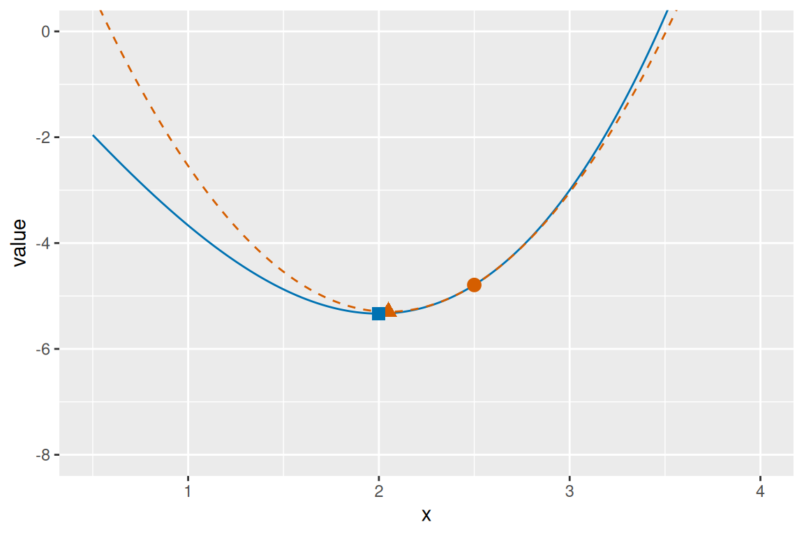
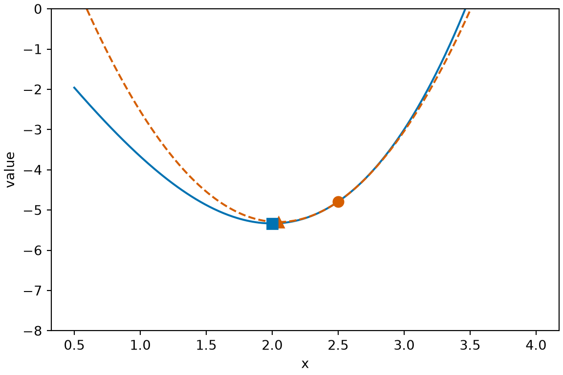
Example 4 (The Newton step at \(x = 2.5\)) For the quadratic approximation \({q\mathopen{}\left(\delta\right)\mathclose{}} = f(2.5) + 2.25\,\delta+ 2.5\,\delta^2\) of Example 3, \(H = [5]\) is positive definite, so by Theorem 1 its minimizer is

\[ \begin{aligned} \delta^* &= -H^{-1} g \\ &= -2.25 / 5 \\ &= -0.45. \end{aligned} \]

Setting the derivative \(2.25 + 5 \delta\) to \(0\) gives the same \(\delta^*\), and

\[ \begin{aligned} 2.5 - 0.45 &= 2.05 \\ &= x^{(1)} \end{aligned} \]

(Example 2).

nm_x_nm <- seq(0.5, 4, length.out = 301)
nm_f_nm <- nm_x_nm^3 / 3 - 4 * nm_x_nm
nm_f0_nm <- 2.5^3 / 3 - 4 * 2.5
nm_q_nm <- nm_f0_nm + 2.25 * (nm_x_nm - 2.5) + 2.5 * (nm_x_nm - 2.5)^2
nm_q_step_nm <- nm_f0_nm + 2.25 * (2.05 - 2.5) + 2.5 * (2.05 - 2.5)^2
nm_f_min_nm <- 2^3 / 3 - 4 * 2
nm_curve_nm <- tibble::tibble(x = nm_x_nm, y = nm_f_nm)
nm_model_nm <- tibble::tibble(x = nm_x_nm, y = nm_q_nm)
nm_start_nm <- tibble::tibble(x = 2.5, y = nm_f0_nm)
nm_step_nm <- tibble::tibble(x = 2.05, y = nm_q_step_nm)
nm_min_nm <- tibble::tibble(x = 2, y = nm_f_min_nm)
nm_aes_nm <- ggplot2::aes(x, y)
nm_ylim_nm <- c(-8, 0)
ggplot2::ggplot(nm_curve_nm, nm_aes_nm) +
  ggplot2::geom_line(colour = "#0072B2") +
  ggplot2::geom_line(
    data = nm_model_nm, colour = "#D55E00", linetype = "dashed"
  ) +
  ggplot2::geom_point(data = nm_start_nm, colour = "#D55E00", size = 3) +
  ggplot2::geom_point(
    data = nm_step_nm, colour = "#D55E00", size = 3, shape = 17
  ) +
  ggplot2::geom_point(
    data = nm_min_nm, colour = "#0072B2", size = 3, shape = 15
  ) +
  ggplot2::coord_cartesian(ylim = nm_ylim_nm) +
  ggplot2::labs(x = "x", y = "value")

import matplotlib.pyplot as plt
import numpy as np

nm_x_fn = np.linspace(0.5, 4, 301)
nm_f_fn = lambda x: x**3 / 3 - 4 * x
nm_q_fn = lambda x: nm_f_fn(2.5) + 2.25 * (x - 2.5) + 2.5 * (x - 2.5) ** 2
fig, ax = plt.subplots(figsize=(6, 4), layout="constrained")
ax.plot(nm_x_fn, nm_f_fn(nm_x_fn), color="#0072B2")
ax.plot(nm_x_fn, nm_q_fn(nm_x_fn), "--", color="#D55E00")
ax.plot(2.5, nm_f_fn(2.5), "o", color="#D55E00", markersize=8)
ax.plot(2.05, nm_q_fn(2.05), "^", color="#D55E00", markersize=8)
ax.plot(2, nm_f_fn(2), "s", color="#0072B2", markersize=8)
ax.set_ylim(-8, 0)
#> (-8.0, 0.0)
ax.set_xlabel("x")
ax.set_ylabel("value")
plt.show();

Figure 1: The cubic \(f(x) = \tfrac{1}{3} x^3 - 4x\) (blue) and its quadratic approximation at \(x = 2.5\) (dashed). The approximation touches \(f\) at \(2.5\) (circle), and its minimizer \(2.05\) (triangle) is the iterate after one Newton step from \(2.5\) (Example 4). It lies close to the minimizer \(2\) of \(f\) (blue marker).

• R
• Python

3 The Newton step as a root of the linear approximation of the gradient

Definition 8 (Linear approximation of the gradient) Let \(f\) be as in Newton’s method and let \(\mathord{\smash[b]{\underset{\raise.3ex\hbox{$\scriptstyle\sim$}}{x}}\vphantom{x}}\) be a point. The linear approximation of the gradient of \(f\) at \(\mathord{\smash[b]{\underset{\raise.3ex\hbox{$\scriptstyle\sim$}}{x}}\vphantom{x}}\) is the \(p \times 1\) vector-valued function \({\mathord{\smash[b]{\underset{\raise.3ex\hbox{$\scriptstyle\sim$}}{g}}\vphantom{g}}_{q}}\) of a step \(\mathord{\smash[b]{\underset{\raise.3ex\hbox{$\scriptstyle\sim$}}{\delta}}\vphantom{\delta}}\in \mathbb{R}^p\) whose \(j\)th entry, for \(j = 1, \ldots, p\), is the function whose graph is the tangent plane to the graph of the partial derivative \(\frac{\partial}{\partial x_j} f\) at \(\mathord{\smash[b]{\underset{\raise.3ex\hbox{$\scriptstyle\sim$}}{x}}\vphantom{x}}\), evaluated at \(\mathord{\smash[b]{\underset{\raise.3ex\hbox{$\scriptstyle\sim$}}{x}}\vphantom{x}}+ \mathord{\smash[b]{\underset{\raise.3ex\hbox{$\scriptstyle\sim$}}{\delta}}\vphantom{\delta}}\):

\[ \mathopen{}\left[{{\mathord{\smash[b]{\underset{\raise.3ex\hbox{$\scriptstyle\sim$}}{g}}\vphantom{g}}_{q}}\mathopen{}\left(\mathord{\smash[b]{\underset{\raise.3ex\hbox{$\scriptstyle\sim$}}{\delta}}\vphantom{\delta}}\right)\mathclose{}}\right]\mathclose{}_j \stackrel{\text{def}}{=}\frac{\partial}{\partial x_j} f(\mathord{\smash[b]{\underset{\raise.3ex\hbox{$\scriptstyle\sim$}}{x}}\vphantom{x}}) + {\mathopen{}\left(\frac{\partial}{\partial \mathord{\smash[b]{\underset{\raise.3ex\hbox{$\scriptstyle\sim$}}{x}}\vphantom{x}}} \mathopen{}\left(\frac{\partial}{\partial x_j} f(\mathord{\smash[b]{\underset{\raise.3ex\hbox{$\scriptstyle\sim$}}{x}}\vphantom{x}})\right)\mathclose{}\right)\mathclose{}}^{\top} \mathord{\smash[b]{\underset{\raise.3ex\hbox{$\scriptstyle\sim$}}{\delta}}\vphantom{\delta}}. \tag{1}\]

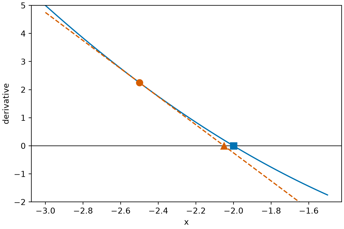
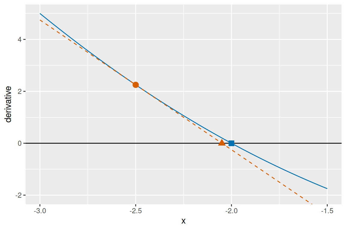
Example 5 (The linear approximation of the derivative of a cubic at \(x = -2.5\)) For \(f(x) = \tfrac{1}{3} x^3 - 4x\), with \(f'(x) = x^2 - 4\) and \(f''(x) = 2x\) (Example 2), \(p = 1\), so the linear approximation of the gradient at \(x = -2.5\) is the tangent line to \(f'\) there:

\[ \begin{aligned} \ell(\delta) &= f'(-2.5) + f''(-2.5)\,\delta && \text{(}\href{#eq-gradient-linear-approximation}{\text{Equation~1}}\text{ with } p = 1 \text{)} \\ &= \mathopen{}\left((-2.5)^2 - 4\right)\mathclose{} + 2 (-2.5)\,\delta && \text{(substitute } f' \text{ and } f'' \text{)} \\ &= 2.25 - 5 \delta. && \text{(arithmetic)} \end{aligned} \tag{2}\]

Figure 2 shows \(f'\) and \(\ell\).

gla_x <- seq(-3, -1.5, length.out = 301)
gla_deriv <- gla_x^2 - 4
gla_line <- 2.25 - 5 * (gla_x + 2.5)
gla_curve <- tibble::tibble(x = gla_x, y = gla_deriv)
gla_tangent <- tibble::tibble(x = gla_x, y = gla_line)
gla_start <- tibble::tibble(x = -2.5, y = 2.25)
gla_step <- tibble::tibble(x = -2.05, y = 0)
gla_root <- tibble::tibble(x = -2, y = 0)
gla_ylim <- c(-2, 5)
gla_curve |>
  ggplot2::ggplot() +
  ggplot2::aes(x = x, y = y) +
  ggplot2::geom_hline(yintercept = 0) +
  ggplot2::geom_line(colour = "#0072B2") +
  ggplot2::geom_line(
    data = gla_tangent, colour = "#D55E00", linetype = "dashed"
  ) +
  ggplot2::geom_point(data = gla_start, colour = "#D55E00", size = 3) +
  ggplot2::geom_point(
    data = gla_step, colour = "#D55E00", size = 3, shape = 17
  ) +
  ggplot2::geom_point(
    data = gla_root, colour = "#0072B2", size = 3, shape = 15
  ) +
  ggplot2::coord_cartesian(ylim = gla_ylim) +
  ggplot2::labs(x = "x", y = "derivative")

import matplotlib.pyplot as plt
import numpy as np

gla_x = np.linspace(-3, -1.5, 301)
fig, ax = plt.subplots(figsize=(6, 4), layout="constrained")
ax.axhline(0, color="black", linewidth=0.8);
ax.plot(gla_x, gla_x**2 - 4, color="#0072B2");
ax.plot(gla_x, 2.25 - 5 * (gla_x + 2.5), "--", color="#D55E00");
ax.plot(-2.5, 2.25, "o", color="#D55E00", markersize=8);
ax.plot(-2.05, 0, "^", color="#D55E00", markersize=8);
ax.plot(-2, 0, "s", color="#0072B2", markersize=8);
ax.set_ylim(-2, 5);
ax.set_xlabel("x");
ax.set_ylabel("derivative");
plt.show();

Figure 2: The derivative \(f'(x) = x^2 - 4\) of the cubic \(f(x) = \tfrac{1}{3} x^3 - 4x\) (blue) and its linear approximation at \(x = -2.5\) (dashed, Equation 2). The tangent line crosses \(0\) at \(-2.05\) (triangle marker), the next Newton iterate, near the root \(-2\) of \(f'\) (square marker).

• R
• Python

Example 6 (The tangent line to \(f\) is not the linear approximation of the gradient) For the cubic \(f(x) = \tfrac{1}{3} x^3 - 4x\) at \(x = -2.5\) (Example 5), the tangent line to \(f\) itself is

\[ \begin{aligned} f(-2.5) + f'(-2.5)\,\delta &= \mathopen{}\left(\tfrac{1}{3} (-2.5)^3 - 4 (-2.5)\right)\mathclose{} + \mathopen{}\left((-2.5)^2 - 4\right)\mathclose{} \delta && \text{(substitute } f \text{ and } f' \text{)} \\ &= \tfrac{115}{24} + 2.25\,\delta. && \text{(arithmetic)} \end{aligned} \tag{3}\]

It is not the linear approximation of the gradient: it approximates \(f\), not \(f'\). Its root, \(\delta= -\tfrac{115}{54}\), is a step toward a zero of \(f\), not toward a stationary point of \(f\).

Lemma 1 (The linear approximation of the gradient uses the Hessian) Let \(f\), \(\mathord{\smash[b]{\underset{\raise.3ex\hbox{$\scriptstyle\sim$}}{x}}\vphantom{x}}\), the gradient \(\mathord{\smash[b]{\underset{\raise.3ex\hbox{$\scriptstyle\sim$}}{g}}\vphantom{g}}\) and the Hessian \(\mathbf{H}\) be as in the quadratic approximation, and let the second partial derivatives of \(f\) be continuous at every point of an open ball around \(\mathord{\smash[b]{\underset{\raise.3ex\hbox{$\scriptstyle\sim$}}{x}}\vphantom{x}}\). Then the linear approximation of the gradient of \(f\) at \(\mathord{\smash[b]{\underset{\raise.3ex\hbox{$\scriptstyle\sim$}}{x}}\vphantom{x}}\) is the gradient plus the Hessian times the step:

\[ {{\mathord{\smash[b]{\underset{\raise.3ex\hbox{$\scriptstyle\sim$}}{g}}\vphantom{g}}_{q}}\mathopen{}\left(\mathord{\smash[b]{\underset{\raise.3ex\hbox{$\scriptstyle\sim$}}{\delta}}\vphantom{\delta}}\right)\mathclose{}} = \mathord{\smash[b]{\underset{\raise.3ex\hbox{$\scriptstyle\sim$}}{g}}\vphantom{g}} + \mathbf{H} \mathord{\smash[b]{\underset{\raise.3ex\hbox{$\scriptstyle\sim$}}{\delta}}\vphantom{\delta}}. \tag{4}\]

Proof. For each \(i\) and \(j\), the \(i\)th entry of \(\frac{\partial}{\partial \mathord{\smash[b]{\underset{\raise.3ex\hbox{$\scriptstyle\sim$}}{x}}\vphantom{x}}} \mathopen{}\left(\frac{\partial}{\partial x_j} f(\mathord{\smash[b]{\underset{\raise.3ex\hbox{$\scriptstyle\sim$}}{x}}\vphantom{x}})\right)\mathclose{}\) is \(\frac{\partial}{\partial x_i} \mathopen{}\left(\frac{\partial}{\partial x_j} f(\mathord{\smash[b]{\underset{\raise.3ex\hbox{$\scriptstyle\sim$}}{x}}\vphantom{x}})\right)\mathclose{}\), which is \(\mathopen{}\left[\mathbf{H}\right]\mathclose{}_{ij}\) by the definitions of the Hessian and of the derivative of a vector-valued function. So, for each \(j\),

\[ \begin{aligned} \mathopen{}\left[{{\mathord{\smash[b]{\underset{\raise.3ex\hbox{$\scriptstyle\sim$}}{g}}\vphantom{g}}_{q}}\mathopen{}\left(\mathord{\smash[b]{\underset{\raise.3ex\hbox{$\scriptstyle\sim$}}{\delta}}\vphantom{\delta}}\right)\mathclose{}}\right]\mathclose{}_j &= \frac{\partial}{\partial x_j} f(\mathord{\smash[b]{\underset{\raise.3ex\hbox{$\scriptstyle\sim$}}{x}}\vphantom{x}}) + \sum_{i=1}^{p} \mathopen{}\left[\mathbf{H}\right]\mathclose{}_{ij}\,\delta_i && \text{(}\href{#eq-gradient-linear-approximation}{\text{Equation~1}}\text{, as a sum)} \\ &= \mathopen{}\left[\mathord{\smash[b]{\underset{\raise.3ex\hbox{$\scriptstyle\sim$}}{g}}\vphantom{g}}\right]\mathclose{}_j + \sum_{i=1}^{p} \mathopen{}\left[\mathbf{H}\right]\mathclose{}_{ij}\,\delta_i && \text{(definition of } \mathord{\smash[b]{\underset{\raise.3ex\hbox{$\scriptstyle\sim$}}{g}}\vphantom{g}} \text{)} \\ &= \mathopen{}\left[\mathord{\smash[b]{\underset{\raise.3ex\hbox{$\scriptstyle\sim$}}{g}}\vphantom{g}}\right]\mathclose{}_j + \sum_{i=1}^{p} \mathopen{}\left[\mathbf{H}\right]\mathclose{}_{ji}\,\delta_i && \text{(} \mathbf{H} \text{ is symmetric)} \\ &= \mathopen{}\left[\mathord{\smash[b]{\underset{\raise.3ex\hbox{$\scriptstyle\sim$}}{g}}\vphantom{g}}\right]\mathclose{}_j + \mathopen{}\left[\mathbf{H} \mathord{\smash[b]{\underset{\raise.3ex\hbox{$\scriptstyle\sim$}}{\delta}}\vphantom{\delta}}\right]\mathclose{}_j && \text{(matrix-vector product)} \\ &= \mathopen{}\left[\mathord{\smash[b]{\underset{\raise.3ex\hbox{$\scriptstyle\sim$}}{g}}\vphantom{g}} + \mathbf{H} \mathord{\smash[b]{\underset{\raise.3ex\hbox{$\scriptstyle\sim$}}{\delta}}\vphantom{\delta}}\right]\mathclose{}_j. && \text{(vector addition)} \end{aligned} \tag{5}\]

The third line uses the symmetry of the Hessian, whose hypothesis the lemma assumes.

Example 7 (A gradient that equals its linear approximation) For \(f(\mathord{\smash[b]{\underset{\raise.3ex\hbox{$\scriptstyle\sim$}}{x}}\vphantom{x}}) = \tfrac{1}{2} (x_1^2 + 3 x_2^2)\), the second function of Example 3, the gradient is \(\mathord{\smash[b]{\underset{\raise.3ex\hbox{$\scriptstyle\sim$}}{g}}\vphantom{g}} = {(x_1,\ 3 x_2)}^{\top}\), and the Hessian is \(\begin{bmatrix} 1 & 0 \\ 0 & 3 \end{bmatrix}\) at every point. By Lemma 1, the linear approximation of the gradient at \(\mathord{\smash[b]{\underset{\raise.3ex\hbox{$\scriptstyle\sim$}}{x}}\vphantom{x}}\) is

\[ \begin{aligned} {{\mathord{\smash[b]{\underset{\raise.3ex\hbox{$\scriptstyle\sim$}}{g}}\vphantom{g}}_{q}}\mathopen{}\left(\mathord{\smash[b]{\underset{\raise.3ex\hbox{$\scriptstyle\sim$}}{\delta}}\vphantom{\delta}}\right)\mathclose{}} &= \begin{bmatrix} x_1 \\ 3 x_2 \end{bmatrix} + \begin{bmatrix} 1 & 0 \\ 0 & 3 \end{bmatrix} \begin{bmatrix} \delta_1 \\ \delta_2 \end{bmatrix} && \text{(}\href{#eq-gradient-linear-approximation-hessian}{\text{Equation~4}}\text{)} \\ &= \begin{bmatrix} x_1 \\ 3 x_2 \end{bmatrix} + \begin{bmatrix} \delta_1 \\ 3 \delta_2 \end{bmatrix} && \text{(matrix-vector product)} \\ &= \begin{bmatrix} x_1 + \delta_1 \\ 3 x_2 + 3 \delta_2 \end{bmatrix} && \text{(vector addition)} \\ &= \begin{bmatrix} x_1 + \delta_1 \\ 3 (x_2 + \delta_2) \end{bmatrix}, && \text{(factor out } 3 \text{)} \end{aligned} \tag{6}\]

which is the gradient of \(f\) at \(\mathord{\smash[b]{\underset{\raise.3ex\hbox{$\scriptstyle\sim$}}{x}}\vphantom{x}}+ \mathord{\smash[b]{\underset{\raise.3ex\hbox{$\scriptstyle\sim$}}{\delta}}\vphantom{\delta}}\): the gradient of this \(f\) is linear, so its linear approximation is exact.

Theorem 2 (The Newton step is the root of the linear approximation of the gradient) Let \(f\), \(\mathord{\smash[b]{\underset{\raise.3ex\hbox{$\scriptstyle\sim$}}{x}}\vphantom{x}}\), \(\mathord{\smash[b]{\underset{\raise.3ex\hbox{$\scriptstyle\sim$}}{g}}\vphantom{g}}\) and the Hessian \(\mathbf{H}\) be as in Lemma 1, with \(\mathbf{H}\) invertible. The only step \(\mathord{\smash[b]{\underset{\raise.3ex\hbox{$\scriptstyle\sim$}}{\delta}}\vphantom{\delta}}\) at which the linear approximation of the gradient is zero is the Newton step:

\[ {{\mathord{\smash[b]{\underset{\raise.3ex\hbox{$\scriptstyle\sim$}}{g}}\vphantom{g}}_{q}}\mathopen{}\left(\mathord{\smash[b]{\underset{\raise.3ex\hbox{$\scriptstyle\sim$}}{\delta}}\vphantom{\delta}}\right)\mathclose{}} = \mathord{\smash[b]{\underset{\raise.3ex\hbox{$\scriptstyle\sim$}}{0}}\vphantom{0}}_{p \times 1} \iff \mathord{\smash[b]{\underset{\raise.3ex\hbox{$\scriptstyle\sim$}}{\delta}}\vphantom{\delta}}= -\mathbf{H}^{-1} \mathord{\smash[b]{\underset{\raise.3ex\hbox{$\scriptstyle\sim$}}{g}}\vphantom{g}}. \tag{7}\]

Proof. By Lemma 1, \({{\mathord{\smash[b]{\underset{\raise.3ex\hbox{$\scriptstyle\sim$}}{g}}\vphantom{g}}_{q}}\mathopen{}\left(\mathord{\smash[b]{\underset{\raise.3ex\hbox{$\scriptstyle\sim$}}{\delta}}\vphantom{\delta}}\right)\mathclose{}} = \mathord{\smash[b]{\underset{\raise.3ex\hbox{$\scriptstyle\sim$}}{0}}\vphantom{0}}_{p \times 1}\) exactly when

\[ \begin{aligned} \mathord{\smash[b]{\underset{\raise.3ex\hbox{$\scriptstyle\sim$}}{0}}\vphantom{0}}_{p \times 1} &= \mathord{\smash[b]{\underset{\raise.3ex\hbox{$\scriptstyle\sim$}}{g}}\vphantom{g}} + \mathbf{H} \mathord{\smash[b]{\underset{\raise.3ex\hbox{$\scriptstyle\sim$}}{\delta}}\vphantom{\delta}} && \text{(}\href{#eq-gradient-linear-approximation-hessian}{\text{Equation~4}}\text{)} \\ -\mathord{\smash[b]{\underset{\raise.3ex\hbox{$\scriptstyle\sim$}}{g}}\vphantom{g}} &= \mathbf{H} \mathord{\smash[b]{\underset{\raise.3ex\hbox{$\scriptstyle\sim$}}{\delta}}\vphantom{\delta}} && \text{(subtract } \mathord{\smash[b]{\underset{\raise.3ex\hbox{$\scriptstyle\sim$}}{g}}\vphantom{g}} \text{ from both sides)} \\ -\mathbf{H}^{-1} \mathord{\smash[b]{\underset{\raise.3ex\hbox{$\scriptstyle\sim$}}{g}}\vphantom{g}} &= \mathord{\smash[b]{\underset{\raise.3ex\hbox{$\scriptstyle\sim$}}{\delta}}\vphantom{\delta}}. && \text{(multiply both sides by } \mathbf{H}^{-1} \text{ on the left)} \end{aligned} \tag{8}\]

Each line implies the next and, because \(\mathbf{H}\) is invertible, the one before, so \(\mathord{\smash[b]{\underset{\raise.3ex\hbox{$\scriptstyle\sim$}}{\delta}}\vphantom{\delta}}= -\mathbf{H}^{-1} \mathord{\smash[b]{\underset{\raise.3ex\hbox{$\scriptstyle\sim$}}{g}}\vphantom{g}}\) is the only solution.

Example 8 (The Newton step at \(x = -2.5\) as a root) At \(x = -2.5\), the linear approximation of the gradient of the cubic \(f(x) = \tfrac{1}{3} x^3 - 4x\) is \(\ell(\delta) = 2.25 - 5 \delta\) (Example 5). Setting it to \(0\),

\[ \begin{aligned} 0 &= 2.25 - 5 \delta && \text{(}\href{#eq-gradient-linear-approximation-cubic}{\text{Equation~2}}\text{)} \\ 5 \delta&= 2.25 && \text{(add } 5 \delta\text{ to both sides)} \\ \delta&= 0.45, && \text{(divide both sides by } 5 \text{)} \end{aligned} \tag{9}\]

so the next iterate is \(-2.5 + 0.45 = -2.05\), the point where the tangent line in Figure 2 crosses \(0\). The Newton’s method iteration \(x^{(t+1)} = \tfrac{1}{2} \mathopen{}\left(x^{(t)} + 4 / x^{(t)}\right)\mathclose{}\) of Example 2 gives the same iterate. Here \(H = [-5]\) is not positive definite, so Theorem 1 does not describe this step, but Theorem 2 does.

Remark 2 (Two ways to read the Newton step). Theorem 1 reads the Newton step as the minimizer of the quadratic approximation, which needs the Hessian \(\mathbf{H}\) to be positive definite. Theorem 2 reads it as the root of the linear approximation of the gradient, which needs only \(\mathbf{H}\) invertible. Newton’s method solves \(\frac{\partial}{\partial \mathord{\smash[b]{\underset{\raise.3ex\hbox{$\scriptstyle\sim$}}{x}}\vphantom{x}}} f(\mathord{\smash[b]{\underset{\raise.3ex\hbox{$\scriptstyle\sim$}}{x}}\vphantom{x}}) = \mathord{\smash[b]{\underset{\raise.3ex\hbox{$\scriptstyle\sim$}}{0}}\vphantom{0}}_{p \times 1}\) by replacing the gradient with its linear approximation at each iterate, so it looks for a stationary point of any kind, not only a minimizer.

4 Convergence

Definition 9 (Quadratic convergence) A sequence \(\mathord{\smash[b]{\underset{\raise.3ex\hbox{$\scriptstyle\sim$}}{x}}\vphantom{x}}^{(0)}, \mathord{\smash[b]{\underset{\raise.3ex\hbox{$\scriptstyle\sim$}}{x}}\vphantom{x}}^{(1)}, \ldots\) in \(\mathbb{R}^p\) that converges to \(\mathord{\smash[b]{\underset{\raise.3ex\hbox{$\scriptstyle\sim$}}{x}}\vphantom{x}}^*\) converges quadratically [4] if there is a constant \(C\) with

\[ \mathopen{}\left\lVert\mathord{\smash[b]{\underset{\raise.3ex\hbox{$\scriptstyle\sim$}}{x}}\vphantom{x}}^{(t+1)} - \mathord{\smash[b]{\underset{\raise.3ex\hbox{$\scriptstyle\sim$}}{x}}\vphantom{x}}^*\right\rVert\mathclose{} \le C\,\mathopen{}\left\lVert\mathord{\smash[b]{\underset{\raise.3ex\hbox{$\scriptstyle\sim$}}{x}}\vphantom{x}}^{(t)} - \mathord{\smash[b]{\underset{\raise.3ex\hbox{$\scriptstyle\sim$}}{x}}\vphantom{x}}^*\right\rVert\mathclose{}^2 \qquad \text{for every } t. \]

Example 9 (Halving the error is not quadratic convergence) \(x^{(t)} = 2^{-t}\) converges to \(0\), but it does not converge quadratically: the bound would need \(2^{-(t+1)} \le C\,(2^{-t})^2 = C\,2^{-2t}\), that is, \(2^{t - 1} \le C\), which fails once \(t > 1 + \log_2 C\). Each step only halves the error.

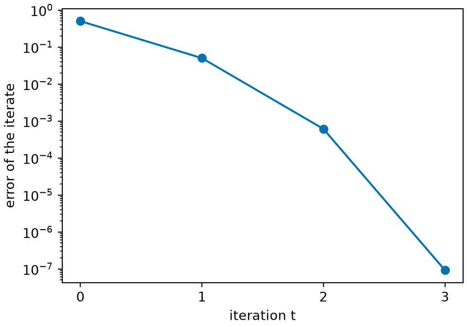
Example 10 (The error squares at each step) For the iteration \(x^{(t+1)} = \tfrac{1}{2} (x^{(t)} + 4 / x^{(t)})\) of Example 2,

\[ \begin{aligned} x^{(t+1)} - 2 &= \frac{1}{2} \mathopen{}\left(x^{(t)} + \frac{4}{x^{(t)}}\right)\mathclose{} - 2 && \text{(the iteration)} \\ &= \frac{(x^{(t)})^2 + 4 - 4 x^{(t)}}{2 x^{(t)}} && \text{(common denominator)} \\ &= \frac{(x^{(t)} - 2)^2}{2 x^{(t)}}. && \text{(the numerator is a perfect square)} \end{aligned} \]

So near \(2\) the error is roughly squared and divided by \(4\) at each step: the errors are \(0.05\), then \(0.00061\), then \(0.000000093\), and \(0.05^2 / (2 \cdot 2.05) \approx 0.00061\). The iterates converge quadratically (Definition 9): \(C = \tfrac{1}{2}\) works for every \(x^{(t)} \ge 1\), since then \(\tfrac{1}{2 x^{(t)}} \le \tfrac{1}{2}\), and every iterate from \(2.5\) is at least \(2\), since the identity makes \(x^{(t+1)} - 2 \ge 0\) whenever \(x^{(t)} > 0\). Zhou [1] states such a bound for Newton’s method in general; it holds from starting points close enough to a minimizer where the Hessian is positive definite, when near that minimizer the Hessian changes by at most a constant times the distance moved, which is not proved here.

nc_x_nc <- numeric(4)
nc_x_nc[1] <- 2.5
for (nc_t_nc in 1:3) {
  nc_prev_nc <- nc_x_nc[nc_t_nc]
  nc_x_nc[nc_t_nc + 1] <- 0.5 * (nc_prev_nc + 4 / nc_prev_nc)
}
nc_steps_nc <- tibble::tibble(t = 0:3, error = nc_x_nc - 2)
ggplot2::ggplot(nc_steps_nc, ggplot2::aes(t, error)) +
  ggplot2::geom_line(colour = "#0072B2") +
  ggplot2::geom_point(colour = "#0072B2", size = 3) +
  ggplot2::scale_y_log10() +
  ggplot2::labs(x = "iteration t", y = "error of the iterate")

import matplotlib.pyplot as plt

nc_x_ax = [2.5]
for _ in range(3):
    nc_x_ax.append(0.5 * (nc_x_ax[-1] + 4 / nc_x_ax[-1]))
nc_err_ax = [x - 2 for x in nc_x_ax]
fig, ax = plt.subplots(figsize=(5, 3.5), layout="constrained")
ax.semilogy(range(4), nc_err_ax, "o-", color="#0072B2")
#> [<matplotlib.lines.Line2D object at 0x7f8eca0ea0d0>]
ax.set_xlabel("iteration t")
#> Text(0.5, 0, 'iteration t')
ax.set_ylabel("error of the iterate")
#> Text(0, 0.5, 'error of the iterate')
ax.set_xticks(range(4))
#> [<matplotlib.axis.XTick object at 0x7f8eca0c3b10>, <matplotlib.axis.XTick object at 0x7f8eca0ea210>, <matplotlib.axis.XTick object at 0x7f8eca0ea990>, <matplotlib.axis.XTick object at 0x7f8eca0eb110>]
plt.show();

Figure 3: The error \(x^{(t)} - 2\) of Example 10 on a logarithmic scale. Each drop is steeper than the one before, because the error is roughly squared at every step, which is quadratic convergence.

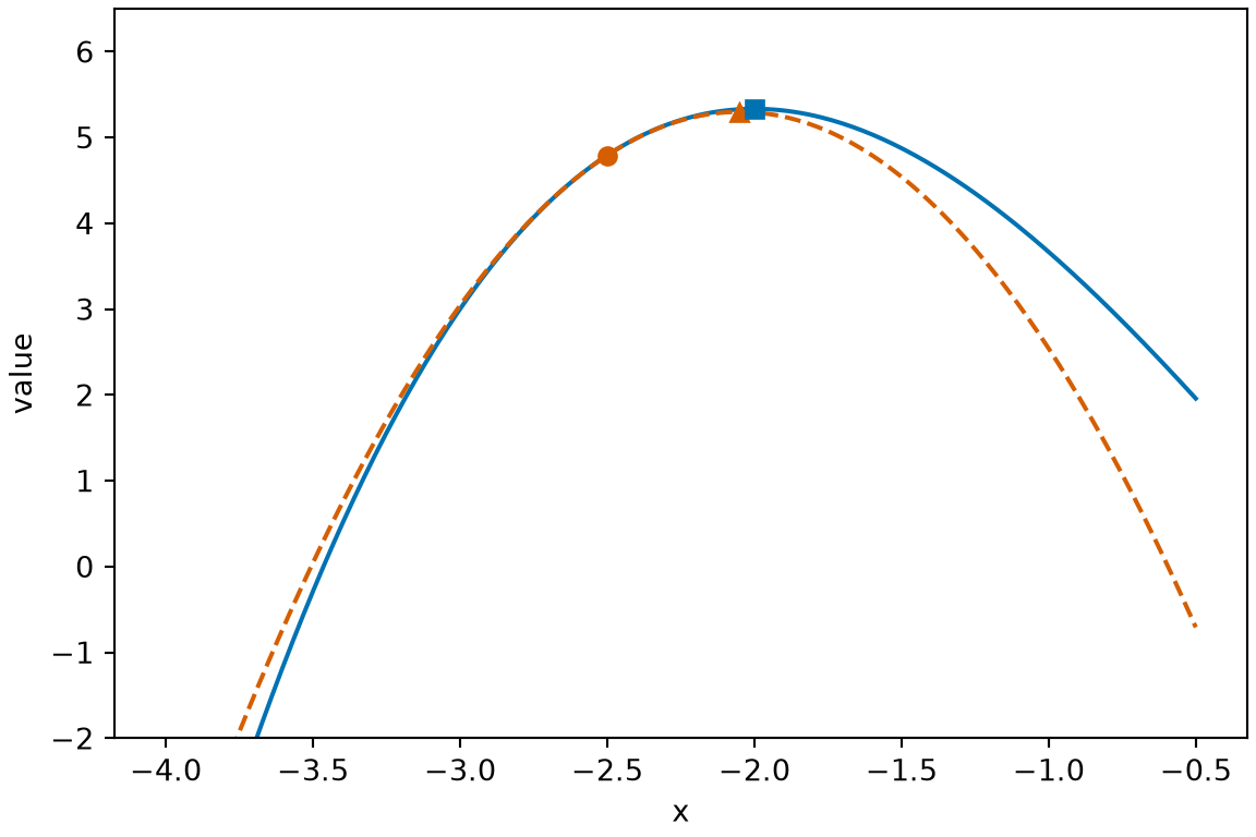
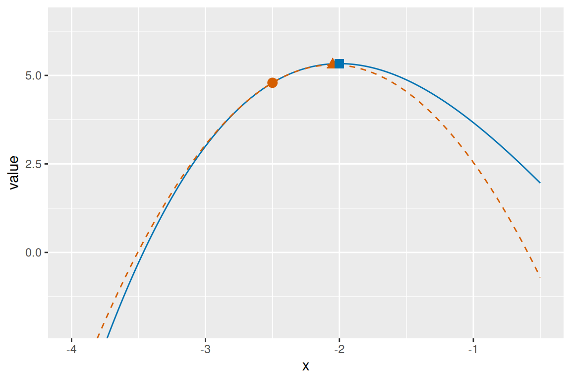
• R
• Python

Example 11 (Newton’s method can find a maximum) From \(x^{(0)} = -2.5\) the same iteration gives \(-2.05\), \(-2.000610\), \(-2.0000001\), approaching \(-2\). But \(-2\) is not a minimizer of \(f\): it is a stationary point of \(-f\), whose second derivative at \(-2\) is \(-f''(-2) = 4 > 0\), so it is a strict local minimizer of \(-f\) (Theorem 7 in Critical Points and Optimality Conditions), that is, \(f\) is strictly larger at \(-2\) than at all nearby points. Newton’s method looks only for a stationary point. In this example, the Hessian \(H = f''(x) = 2x\) is negative at every iterate. If \(H < 0\), then Theorem 1 does not apply, because it requires a positive definite Hessian. Instead, the quadratic approximation \({q\mathopen{}\left(\delta\right)\mathclose{}} = f + g\,\delta+ \tfrac{1}{2} H \delta^2\) tends to \(-\infty\) as \(\mathopen{}\left|\delta\right|\mathclose{} \to \infty\), so it has no minimizer.

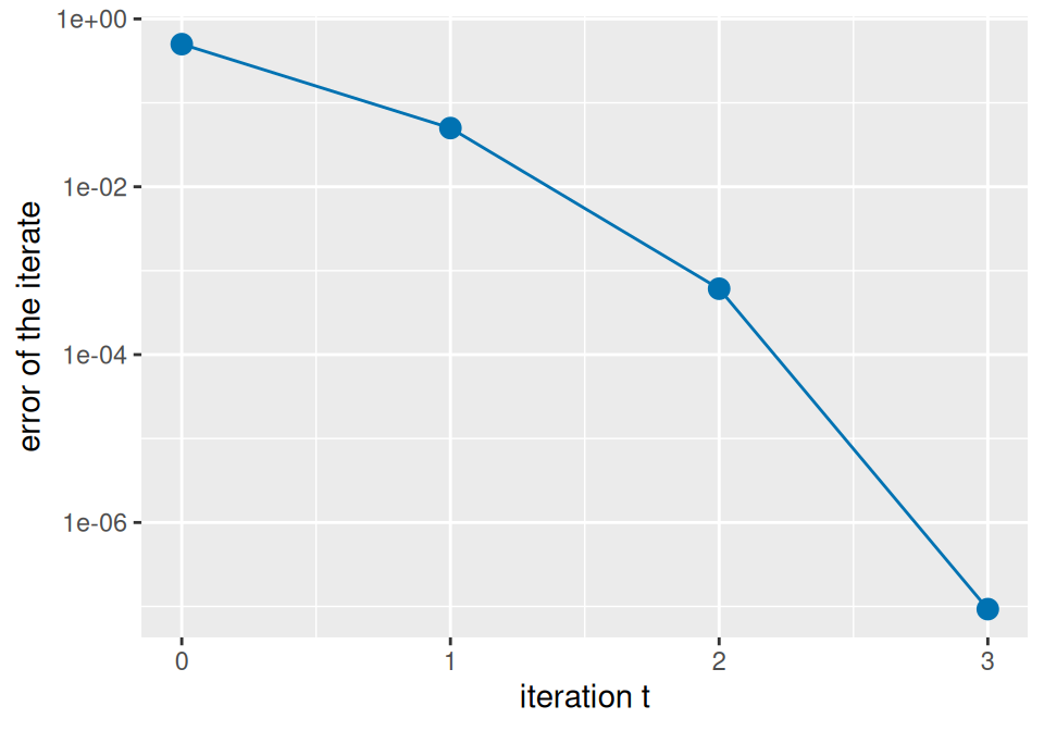
Figure 4 shows the cubic and its quadratic approximation.

nx_x_nx <- seq(-4, -0.5, length.out = 301)
nx_f_nx <- nx_x_nx^3 / 3 - 4 * nx_x_nx
nx_f0_nx <- (-2.5)^3 / 3 - 4 * (-2.5)
nx_dx_nx <- nx_x_nx + 2.5
nx_q_nx <- nx_f0_nx + 2.25 * nx_dx_nx - 2.5 * nx_dx_nx^2
nx_dstep_nx <- -2.05 + 2.5
nx_q_step_nx <- nx_f0_nx + 2.25 * nx_dstep_nx - 2.5 * nx_dstep_nx^2
nx_f_max_nx <- (-2)^3 / 3 - 4 * (-2)
nx_curve_nx <- tibble::tibble(x = nx_x_nx, y = nx_f_nx)
nx_model_nx <- tibble::tibble(x = nx_x_nx, y = nx_q_nx)
nx_start_nx <- tibble::tibble(x = -2.5, y = nx_f0_nx)
nx_step_nx <- tibble::tibble(x = -2.05, y = nx_q_step_nx)
nx_max_nx <- tibble::tibble(x = -2, y = nx_f_max_nx)
nx_aes_nx <- ggplot2::aes(x, y)
nx_ylim_nx <- c(-2, 6.5)
nx_curve_nx |>
  ggplot2::ggplot() +
  nx_aes_nx +
  ggplot2::geom_line(colour = "#0072B2") +
  ggplot2::geom_line(
    data = nx_model_nx, colour = "#D55E00", linetype = "dashed"
  ) +
  ggplot2::geom_point(data = nx_start_nx, colour = "#D55E00", size = 3) +
  ggplot2::geom_point(
    data = nx_step_nx, colour = "#D55E00", size = 3, shape = 17
  ) +
  ggplot2::geom_point(
    data = nx_max_nx, colour = "#0072B2", size = 3, shape = 15
  ) +
  ggplot2::coord_cartesian(ylim = nx_ylim_nx) +
  ggplot2::labs(x = "x", y = "value")

import matplotlib.pyplot as plt
import numpy as np

nx_x_py = np.linspace(-4, -0.5, 301)
nx_f_py = nx_x_py**3 / 3 - 4 * nx_x_py
nx_f0_py = (-2.5)**3 / 3 - 4 * (-2.5)
nx_q_py = nx_f0_py + 2.25 * (nx_x_py + 2.5) - 2.5 * (nx_x_py + 2.5)**2
nx_q_step_py = nx_f0_py + 2.25 * (-2.05 + 2.5) - 2.5 * (-2.05 + 2.5)**2
nx_f_max_py = (-2)**3 / 3 - 4 * (-2)
fig, ax = plt.subplots(figsize=(6, 4), layout="constrained")
ax.plot(nx_x_py, nx_f_py, color="#0072B2")
#> [<matplotlib.lines.Line2D object at 0x7f8eca1ef750>]
ax.plot(nx_x_py, nx_q_py, "--", color="#D55E00")
#> [<matplotlib.lines.Line2D object at 0x7f8eca1ef4d0>]
ax.plot([-2.5], [nx_f0_py], "o", color="#D55E00")
#> [<matplotlib.lines.Line2D object at 0x7f8eca1ef390>]
ax.plot([-2.05], [nx_q_step_py], "^", color="#D55E00")
#> [<matplotlib.lines.Line2D object at 0x7f8eca1ee210>]
ax.plot([-2], [nx_f_max_py], "s", color="#0072B2")
#> [<matplotlib.lines.Line2D object at 0x7f8eca1efb10>]
ax.set_ylim(-2, 6.5)
#> (-2.0, 6.5)
ax.set_xlabel("x")
#> Text(0.5, 0, 'x')
ax.set_ylabel("value")
#> Text(0, 0.5, 'value')
plt.show();

Figure 4: The cubic \(f(x) = x^3 / 3 - 4x\) of Example 11 is blue, and its quadratic approximation at the start \(-2.5\) is dashed vermilion. The approximation opens downward, so its stationary point \(-2.05\) (triangle) is the point where the approximation is largest, and the Newton step moves uphill. The iterates approach the local maximum at \(-2\) (blue marker).

• R
• Python

Theorem 3 (Newton’s method minimizes a quadratic in one step) Let \(\mathbf{S}\) be a \(p \times p\) positive definite matrix, \(\mathord{\smash[b]{\underset{\raise.3ex\hbox{$\scriptstyle\sim$}}{c}}\vphantom{c}} \in \mathbb{R}^p\), and \(f(\mathord{\smash[b]{\underset{\raise.3ex\hbox{$\scriptstyle\sim$}}{x}}\vphantom{x}}) = \tfrac{1}{2}\,{\mathord{\smash[b]{\underset{\raise.3ex\hbox{$\scriptstyle\sim$}}{x}}\vphantom{x}}}^{\top} \mathbf{S} \mathord{\smash[b]{\underset{\raise.3ex\hbox{$\scriptstyle\sim$}}{x}}\vphantom{x}} - \mathord{\smash[b]{\underset{\raise.3ex\hbox{$\scriptstyle\sim$}}{c}}\vphantom{c}} \cdot \mathord{\smash[b]{\underset{\raise.3ex\hbox{$\scriptstyle\sim$}}{x}}\vphantom{x}}\). From any \(\mathord{\smash[b]{\underset{\raise.3ex\hbox{$\scriptstyle\sim$}}{x}}\vphantom{x}}^{(0)}\), Newton’s method (Definition 5) gives \(\mathord{\smash[b]{\underset{\raise.3ex\hbox{$\scriptstyle\sim$}}{x}}\vphantom{x}}^{(1)} = \mathbf{S}^{-1} \mathord{\smash[b]{\underset{\raise.3ex\hbox{$\scriptstyle\sim$}}{c}}\vphantom{c}}\), the unique minimizer of \(f\).

Proof. Partial derivatives of a sum or of a constant multiple are the sum or multiple of the partial derivatives, so the derivative of a quadratic form applies to \(\tfrac{1}{2}\,{\mathord{\smash[b]{\underset{\raise.3ex\hbox{$\scriptstyle\sim$}}{x}}\vphantom{x}}}^{\top} \mathbf{S} \mathord{\smash[b]{\underset{\raise.3ex\hbox{$\scriptstyle\sim$}}{x}}\vphantom{x}}\) and the derivative of a linear combination to \(\mathord{\smash[b]{\underset{\raise.3ex\hbox{$\scriptstyle\sim$}}{c}}\vphantom{c}} \cdot \mathord{\smash[b]{\underset{\raise.3ex\hbox{$\scriptstyle\sim$}}{x}}\vphantom{x}}\):

\[ \begin{aligned} \frac{\partial}{\partial \mathord{\smash[b]{\underset{\raise.3ex\hbox{$\scriptstyle\sim$}}{x}}\vphantom{x}}} f(\mathord{\smash[b]{\underset{\raise.3ex\hbox{$\scriptstyle\sim$}}{x}}\vphantom{x}}) &= \tfrac{1}{2} (2 \mathbf{S} \mathord{\smash[b]{\underset{\raise.3ex\hbox{$\scriptstyle\sim$}}{x}}\vphantom{x}}) - \mathord{\smash[b]{\underset{\raise.3ex\hbox{$\scriptstyle\sim$}}{c}}\vphantom{c}} \\ &= \mathbf{S} \mathord{\smash[b]{\underset{\raise.3ex\hbox{$\scriptstyle\sim$}}{x}}\vphantom{x}}- \mathord{\smash[b]{\underset{\raise.3ex\hbox{$\scriptstyle\sim$}}{c}}\vphantom{c}}; \end{aligned} \]

by the Hessian of a quadratic form with \(\tfrac{1}{2} \mathbf{S}\) in place of \(\mathbf{S}\), and because the gradient \(-\mathord{\smash[b]{\underset{\raise.3ex\hbox{$\scriptstyle\sim$}}{c}}\vphantom{c}}\) of the linear term is constant, \(\mathbf{H}_f(\mathord{\smash[b]{\underset{\raise.3ex\hbox{$\scriptstyle\sim$}}{x}}\vphantom{x}}) = \mathbf{S}\), which is invertible. So

\[ \begin{aligned} \mathord{\smash[b]{\underset{\raise.3ex\hbox{$\scriptstyle\sim$}}{x}}\vphantom{x}}^{(1)} &= \mathord{\smash[b]{\underset{\raise.3ex\hbox{$\scriptstyle\sim$}}{x}}\vphantom{x}}^{(0)} - \mathbf{S}^{-1} (\mathbf{S} \mathord{\smash[b]{\underset{\raise.3ex\hbox{$\scriptstyle\sim$}}{x}}\vphantom{x}}^{(0)} - \mathord{\smash[b]{\underset{\raise.3ex\hbox{$\scriptstyle\sim$}}{c}}\vphantom{c}}) && \text{(definition of Newton's method)} \\ &= \mathord{\smash[b]{\underset{\raise.3ex\hbox{$\scriptstyle\sim$}}{x}}\vphantom{x}}^{(0)} - \mathbf{S}^{-1} \mathbf{S} \mathord{\smash[b]{\underset{\raise.3ex\hbox{$\scriptstyle\sim$}}{x}}\vphantom{x}}^{(0)} + \mathbf{S}^{-1} \mathord{\smash[b]{\underset{\raise.3ex\hbox{$\scriptstyle\sim$}}{c}}\vphantom{c}} && \text{(distribute)} \\ &= \mathord{\smash[b]{\underset{\raise.3ex\hbox{$\scriptstyle\sim$}}{x}}\vphantom{x}}^{(0)} - \mathord{\smash[b]{\underset{\raise.3ex\hbox{$\scriptstyle\sim$}}{x}}\vphantom{x}}^{(0)} + \mathbf{S}^{-1} \mathord{\smash[b]{\underset{\raise.3ex\hbox{$\scriptstyle\sim$}}{c}}\vphantom{c}} && \text{(} \mathbf{S}^{-1} \mathbf{S} = \mathbf{I}_p \text{)} \\ &= \mathbf{S}^{-1} \mathord{\smash[b]{\underset{\raise.3ex\hbox{$\scriptstyle\sim$}}{c}}\vphantom{c}}. && \text{(cancel)} \end{aligned} \]

The gradient at \(\mathbf{S}^{-1} \mathord{\smash[b]{\underset{\raise.3ex\hbox{$\scriptstyle\sim$}}{c}}\vphantom{c}}\) is \(\mathbf{S} \mathbf{S}^{-1} \mathord{\smash[b]{\underset{\raise.3ex\hbox{$\scriptstyle\sim$}}{c}}\vphantom{c}} - \mathord{\smash[b]{\underset{\raise.3ex\hbox{$\scriptstyle\sim$}}{c}}\vphantom{c}} = \mathord{\smash[b]{\underset{\raise.3ex\hbox{$\scriptstyle\sim$}}{0}}\vphantom{0}}_{p \times 1}\), and \(f\) is strictly convex (Theorem 6 in Convexity in Several Variables, part 2), so \(\mathbf{S}^{-1} \mathord{\smash[b]{\underset{\raise.3ex\hbox{$\scriptstyle\sim$}}{c}}\vphantom{c}}\) is a global minimizer (Corollary 2 in Convexity in Several Variables). It is the only one: a strictly convex function has at most one global minimizer, since the midpoint of two distinct global minimizers, which have equal values, would have a strictly smaller value (Definition 4 in Convexity in Several Variables with \(t = \tfrac{1}{2}\)).

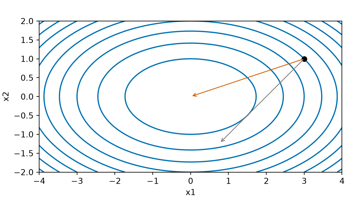
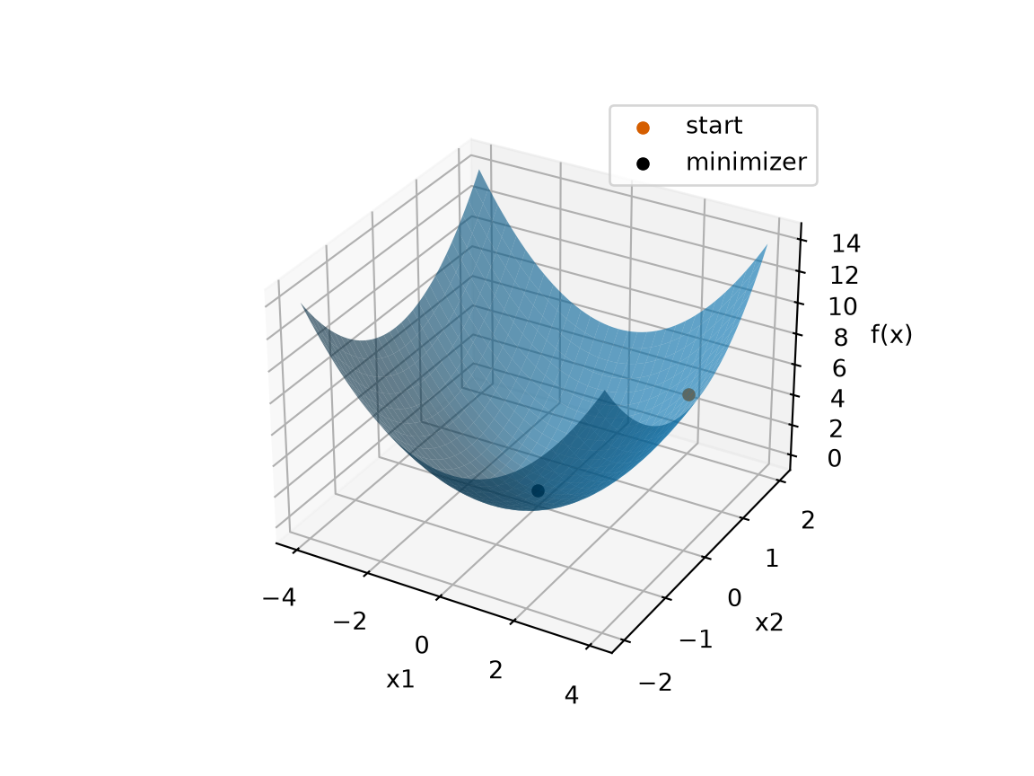
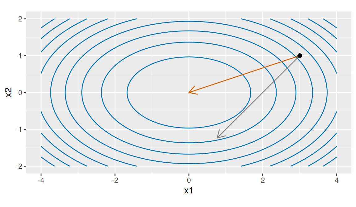
Example 12 (One step to the minimizer) Let \(f(\mathord{\smash[b]{\underset{\raise.3ex\hbox{$\scriptstyle\sim$}}{x}}\vphantom{x}}) = \tfrac{1}{2} (x_1^2 + 3 x_2^2)\), so \(\mathbf{S} = \begin{bmatrix} 1 & 0 \\ 0 & 3 \end{bmatrix}\) and \(\mathord{\smash[b]{\underset{\raise.3ex\hbox{$\scriptstyle\sim$}}{c}}\vphantom{c}} = \mathord{\smash[b]{\underset{\raise.3ex\hbox{$\scriptstyle\sim$}}{0}}\vphantom{0}}_{2 \times 1}\). From \(\mathord{\smash[b]{\underset{\raise.3ex\hbox{$\scriptstyle\sim$}}{x}}\vphantom{x}}^{(0)} = {(3, 1)}^{\top}\) the gradient is \(\nabla f(\mathord{\smash[b]{\underset{\raise.3ex\hbox{$\scriptstyle\sim$}}{x}}\vphantom{x}}^{(0)}) = \mathbf{S} \mathord{\smash[b]{\underset{\raise.3ex\hbox{$\scriptstyle\sim$}}{x}}\vphantom{x}}^{(0)} = {(3, 3)}^{\top}\), and \(\mathbf{S}^{-1} = \begin{bmatrix} 1 & 0 \\ 0 & 1/3 \end{bmatrix}\), so the Newton step is \(-\mathbf{S}^{-1} {(3, 3)}^{\top} = -{(3, 1)}^{\top}\) and

\[ \begin{aligned} \mathord{\smash[b]{\underset{\raise.3ex\hbox{$\scriptstyle\sim$}}{x}}\vphantom{x}}^{(1)} &= {(3, 1)}^{\top} - {(3, 1)}^{\top} \\ &= \mathord{\smash[b]{\underset{\raise.3ex\hbox{$\scriptstyle\sim$}}{0}}\vphantom{0}}_{2 \times 1}, \end{aligned} \]

the minimizer.

Figure 5 shows the step on the level curves of \(f\).

nq_x1_nq <- seq(-4, 4, length.out = 101)
nq_x2_nq <- seq(-2, 2, length.out = 101)
nq_grid_nq <- tidyr::expand_grid(x1 = nq_x1_nq, x2 = nq_x2_nq)
nq_grid_nq$z <- (nq_grid_nq$x1^2 + 3 * nq_grid_nq$x2^2) / 2
nq_newton_nq <- tibble::tibble(x = 3, y = 1, xend = 0, yend = 0)
nq_grad_nq <- tibble::tibble(x = 3, y = 1, xend = 0.764, yend = -1.236)
nq_start_nq <- tibble::tibble(x1 = 3, x2 = 1)
nq_head_nq <- grid::unit(0.15, "inches")
nq_arrow_nq <- grid::arrow(length = nq_head_nq)
nq_aes_nq <- ggplot2::aes(x1, x2)
nq_z_aes_nq <- ggplot2::aes(z = z)
nq_seg_aes_nq <- ggplot2::aes(x = x, y = y, xend = xend, yend = yend)
nq_grid_nq |>
  ggplot2::ggplot() +
  nq_aes_nq +
  ggplot2::geom_contour(nq_z_aes_nq, colour = "#0072B2", bins = 10) +
  ggplot2::geom_segment(
    nq_seg_aes_nq,
    data = nq_grad_nq,
    colour = "grey50",
    arrow = nq_arrow_nq
  ) +
  ggplot2::geom_segment(
    nq_seg_aes_nq,
    data = nq_newton_nq,
    colour = "#D55E00",
    arrow = nq_arrow_nq
  ) +
  ggplot2::geom_point(data = nq_start_nq, size = 2) +
  ggplot2::coord_fixed() +
  ggplot2::labs(x = "x1", y = "x2")

import matplotlib.pyplot as plt
import numpy as np

nq_xx_py, nq_yy_py = np.meshgrid(np.linspace(-4, 4, 101),
                                 np.linspace(-2, 2, 101))
nq_z_py = (nq_xx_py**2 + 3 * nq_yy_py**2) / 2
fig, ax = plt.subplots(figsize=(6, 3.5), layout="constrained")
ax.contour(nq_xx_py, nq_yy_py, nq_z_py, levels=10, colors="#0072B2")
#> <matplotlib.contour.QuadContourSet object at 0x7f8ed83bdd30>
ax.annotate("", xy=(0.764, -1.236), xytext=(3, 1),
            arrowprops={"arrowstyle": "->", "color": "grey"})
#> Text(3, 1, '')
ax.annotate("", xy=(0, 0), xytext=(3, 1),
            arrowprops={"arrowstyle": "->", "color": "#D55E00"})
#> Text(3, 1, '')
ax.plot([3], [1], "ko")
#> [<matplotlib.lines.Line2D object at 0x7f8ec7dae710>]
ax.set_aspect("equal")
ax.set_xlabel("x1")
#> Text(0.5, 0, 'x1')
ax.set_ylabel("x2")
#> Text(0, 0.5, 'x2')
plt.show();

Figure 5: The level curves of \(f\) in Example 12 are ellipses. From the start \({(3, 1)}^{\top}\), the Newton step (vermilion arrow) goes straight to the minimizer at the origin. The negative gradient \(-{(3, 3)}^{\top}\) (grey arrow, drawn as long as the Newton step) points across the narrow side of the ellipses and misses the origin.

• R
• Python

Figure 6 shows the same function as a surface.

nq_x1_sf <- seq(-4, 4, length.out = 61)
nq_x2_sf <- seq(-2, 2, length.out = 61)
nq_grid_sf <- tidyr::expand_grid(x1 = nq_x1_sf, x2 = nq_x2_sf)
nq_value_sf <- (nq_grid_sf$x1^2 + 3 * nq_grid_sf$x2^2) / 2
nq_n2_sf <- length(nq_x2_sf)
nq_z_sf <- matrix(nq_value_sf, nrow = nq_n2_sf)
nq_start_sf <- tibble::tibble(x1 = 3, x2 = 1, z = 6)
nq_min_sf <- tibble::tibble(x1 = 0, x2 = 0, z = 0)
nq_red_sf <- list(color = "#D55E00", size = 5)
nq_black_sf <- list(color = "#000000", size = 5)
nq_stops_sf <- c(0, 1)
nq_cols_sf <- c("#CCE0F0", "#0072B2")
nq_scale_sf <- list(nq_stops_sf, nq_cols_sf)
nq_eye_sf <- list(x = 1.6, y = -1.6, z = 0.9)
nq_camera_sf <- list(eye = nq_eye_sf)
nq_xaxis_sf <- list(title = "x1")
nq_yaxis_sf <- list(title = "x2")
nq_zaxis_sf <- list(title = "f(x)")
nq_scene_sf <- list(
  xaxis = nq_xaxis_sf,
  yaxis = nq_yaxis_sf,
  zaxis = nq_zaxis_sf,
  camera = nq_camera_sf
)
nq_legend_sf <- list(orientation = "h")
plotly::plot_ly() |>
  plotly::add_surface(
    x = nq_x1_sf,
    y = nq_x2_sf,
    z = nq_z_sf,
    colorscale = nq_scale_sf,
    showscale = FALSE,
    opacity = 0.8
  ) |>
  plotly::add_trace(
    data = nq_start_sf,
    x = ~x1,
    y = ~x2,
    z = ~z,
    type = "scatter3d",
    mode = "markers",
    marker = nq_red_sf,
    name = "start"
  ) |>
  plotly::add_trace(
    data = nq_min_sf,
    x = ~x1,
    y = ~x2,
    z = ~z,
    type = "scatter3d",
    mode = "markers",
    marker = nq_black_sf,
    name = "minimizer"
  ) |>
  plotly::layout(scene = nq_scene_sf, legend = nq_legend_sf)

import matplotlib.pyplot as plt
import numpy as np

nq_x1_3d, nq_x2_3d = np.meshgrid(np.linspace(-4, 4, 61),
                                 np.linspace(-2, 2, 61))
nq_z_3d = (nq_x1_3d**2 + 3 * nq_x2_3d**2) / 2
fig = plt.figure(figsize=(6, 4.5))
ax = fig.add_subplot(projection="3d")
ax.plot_surface(nq_x1_3d, nq_x2_3d, nq_z_3d, color="#0072B2", alpha=0.6)
#> <mpl_toolkits.mplot3d.art3d.Poly3DCollection object at 0x7f8eca1cb4d0>
ax.scatter([3], [1], [6], color="#D55E00", label="start")
#> <mpl_toolkits.mplot3d.art3d.Path3DCollection object at 0x7f8eca1cb620>
ax.scatter([0], [0], [0], color="black", label="minimizer")
#> <mpl_toolkits.mplot3d.art3d.Path3DCollection object at 0x7f8ec7ba6c10>
ax.set_xlabel("x1")
#> Text(0.5, 0, 'x1')
ax.set_ylabel("x2")
#> Text(0.5, 0.5, 'x2')
ax.set_zlabel("f(x)")
#> Text(0.5, 0, 'f(x)')
ax.legend(loc="upper right")
#> <matplotlib.legend.Legend object at 0x7f8eca1cb770>
plt.show();

Figure 6: The graph of \(f\) in Example 12 is a bowl whose lowest point is the origin.

• R
• Python

[1]

H. Zhou, “Optimization and multivariate calculus.” Lecture notes for Biostat 216, Mathematical Methods for Biostatistics, University of California, Los Angeles, 2024. Accessed: Oct. 05, 2026. [Online]. Available: https://ucla-biostat-216.github.io/2024fall/slides/13-optim/13-optim.html

[2]

Wikipedia contributors, “Iterative method — Wikipedia, the free encyclopedia.” 2026. Available: https://en.wikipedia.org/wiki/Iterative_method

[3]

Wikipedia contributors, “Newton’s method in optimization — Wikipedia, the free encyclopedia.” 2026. Available: https://en.wikipedia.org/wiki/Newton%27s_method_in_optimization

[4]

Wikipedia contributors, “Rate of convergence — Wikipedia, the free encyclopedia.” 2026. Available: https://en.wikipedia.org/wiki/Rate_of_convergence