Definition 2 (Polynomial) A polynomial (in one variable \(x\)) [1] is a function\(f : \mathbb{R}\to \mathbb{R}\) that can be written as \[
f(x) = a_n x^n + a_{n-1} x^{n-1} + \cdots + a_1 x + a_0
\] for some integer \(n \ge 0\) and constants \(a_0, a_1, \ldots, a_n \in \mathbb{R}\) with \(a_n \ne 0\). The terms of \(f\) are \(a_n x^n, \ldots, a_1 x, a_0\).
Remark 1 (Constant and zero polynomials). A constant function\(f(x) = 7\) is a polynomial with \(n = 0\) and \(a_0 = 7\). The requirement \(a_n \ne 0\) means this definition covers nonzero polynomials only: the zero function \(f(x) = 0\) is excluded here, because it has no nonzero coefficient to serve as \(a_n\).
Definition 3 (Coefficients of a polynomial) The constants \(a_0, a_1, \ldots, a_n\) of a polynomial \(f\) (Definition 2) are the coefficients of \(f\), with \(a_k\) the coefficient of \(x^k\).
Definition 4 (Degree of a polynomial) Let \(f(x) = a_n x^n + \cdots + a_1 x + a_0\) be a polynomial with \(a_n \ne 0\). The integer \(n\) is the degree of \(f\).
Definition 5 (Leading coefficient) Let \(f(x) = a_n x^n + \cdots + a_1 x + a_0\) be a polynomial of degree\(n\). The constant \(a_n\) is the leading coefficient of \(f\).
Example 5 (The parabola \(y = x^2\)) The graph of \(f(x) = x^2\) is a parabola. It contains the points \((-1, 1)\), \((0, 0)\) and \((2, 4)\), and its lowest point is \((0, 0)\), since \(x^2 \ge 0\) for every \(x\).
Definition 10 (Degree of a monomial) The degree of the monomial\(x_1^{a_1} x_2^{a_2} \cdots x_p^{a_p}\) is the sum of its exponents, \(a_1 + a_2 + \cdots + a_p\)[4].
Definition 13 (Intercept, y-intercept) The intercept (or y-intercept) of a function\(f\) whose domain contains \(0\) is \(f(0)\), the height at which the graph of \(f\) crosses the vertical axis.
Definition 14 (Intercept term) When a function is written as terms added together, its intercept term is the term with no factor of the input. When every other term has a factor of the input, the intercept (Definition 13) of the function is this term.
Definition 15 (x-intercept) An x-intercept of a function\(f\) is an input\(x\) with \(f(x) = 0\), a point where the graph of \(f\) crosses the horizontal axis. A function can have no x-intercept, one, or many.
Definition 16 (Linear function of one variable) A function \(f: \mathbb{R}\to \mathbb{R}\) is linear[7] if it is affine (Definition 11) with intercept \(0\); that is, if there is a number \(m\) such that
\[f(x) = m x \quad \text{for all } x \in \mathbb{R}\]
LemTheorem 1 (Intercept and slope of an affine function)
Theorem 1 (Intercept and slope of an affine function) Let \(f(x) = m x + b\) be an affine function (Definition 11).
The intercept is the value at zero: \(f(0) = b\).
The slope is the change in \(f\) per unit change in \(x\): for any \(x_1 \neq x_2\), \[\frac{f(x_2) - f(x_1)}{x_2 - x_1} = m\]
So \(f\) determines its slope and intercept: if also \(f(x) = m' x + b'\) for all \(x\), then \(m' = m\) and \(b' = b\).
ProofProof
Proof. Part 1.
\[
\begin{aligned}
f(0)
&= m \cdot 0 + b
&& \text{(}\href{#def-affine-function}{\text{Definition~11}}\text{)}
\\&= 0 + b
&& \text{(any number times } 0 \text{ is } 0 \text{)}
\\&= b + 0
&& \text{(}\href{algebra-sums.qmd#thm-sum-symmetric}{\text{Theorem~5 in Convexity, Infimum and Sums}}\text{)}
\\&= b
&& \text{(}\href{algebra-sums.qmd#thm-add-ident}{\text{Theorem~4 in Convexity, Infimum and Sums}}\text{)}
\end{aligned}
\]
Part 2. First the numerator:
\[
\begin{aligned}
f(x_2) - f(x_1)
&= (m x_2 + b) - (m x_1 + b)
&& \text{(}\href{#def-affine-function}{\text{Definition~11}}\text{)}
\\&= m x_2 + b - m x_1 - b
&& \text{(subtracting a sum subtracts each term)}
\\&= m x_2 - m x_1 + b - b
&& \text{(}\href{algebra-sums.qmd#thm-sum-symmetric}{\text{Theorem~5 in Convexity, Infimum and Sums}}\text{, swapping } b \text{ and } {-m x_1} \text{)}
\\&= (m x_2 - m x_1) + (b - b)
&& \text{(}\href{algebra-sums.qmd#thm-sum-assoc}{\text{Theorem~6 in Convexity, Infimum and Sums}}\text{)}
\\&= (m x_2 - m x_1) + 0
&& (b - b = 0)
\\&= m x_2 - m x_1
&& \text{(}\href{algebra-sums.qmd#thm-add-ident}{\text{Theorem~4 in Convexity, Infimum and Sums}}\text{)}
\\&= m x_2 + m (-x_1)
&& (-(m x_1) = m (-x_1) \text{, by }\href{algebra-basics.qmd#thm-negative-one}{\text{Theorem~6 in Equalities, Inequalities and Minimizers}}\text{ and }\href{algebra-sums.qmd#thm-prod-assoc}{\text{Theorem~9 in Convexity, Infimum and Sums}}\text{)}
\\&= m (x_2 + (-x_1))
&& \text{(}\href{algebra-sums.qmd#thm-mult-distr}{\text{Theorem~11 in Convexity, Infimum and Sums}}\text{, read right to left)}
\\&= m (x_2 - x_1)
&& \text{(adding a negative is subtracting)}
\end{aligned}
\]
Then, writing \(d = x_2 - x_1\), which is not \(0\) because \(x_1 \neq x_2\),
\[
\begin{aligned}
\frac{f(x_2) - f(x_1)}{x_2 - x_1}
&= \frac{m d}{d}
&& \text{(the numerator above)}
\\&= (m d) \cdot\frac{1}{d}
&& \text{(}\href{algebra-sums.qmd#thm-prod-div}{\text{Theorem~10 in Convexity, Infimum and Sums}}\text{)}
\\&= m \cdot\mathopen{}\left(d \cdot\frac{1}{d}\right)\mathclose{}
&& \text{(}\href{algebra-sums.qmd#thm-prod-assoc}{\text{Theorem~9 in Convexity, Infimum and Sums}}\text{)}
\\&= m \cdot\frac{d}{d}
&& \text{(}\href{algebra-sums.qmd#thm-prod-div}{\text{Theorem~10 in Convexity, Infimum and Sums}}\text{)}
\\&= m \cdot 1
&& \text{(a nonzero number divided by itself is } 1 \text{)}
\\&= m
&& \text{(}\href{algebra-sums.qmd#thm-mult-one}{\text{Theorem~7 in Convexity, Infimum and Sums}}\text{)}
\end{aligned}
\]
Part 3. Part 1, applied to each formula, gives
\[
\begin{aligned}
b &= f(0) \\
&= b'.
\end{aligned}
\]
Part 2 with \(x_1 = 0\) and \(x_2 = 1\), applied to each formula, gives
ExmExample 8 (An affine function, and a linear one)
Example 8 (An affine function, and a linear one)\(f(x) = 2x + 3\) is affine with slope \(2\) and intercept \(3\). By Theorem 1, \(f(0) = 3\), and each unit step in \(x\) raises \(f\) by \(2\): for example, \(f(1) = 5\) and \(f(2) = 7\). Its intercept is not \(0\), so it is not linear.
\(g(x) = -\tfrac{1}{2} x\) is affine with intercept \(0\), so it is linear: \(g(0) = 0\), and each unit step in \(x\) lowers \(g\) by \(\tfrac{1}{2}\).
RemarkRemark 3 (Elementary algebra calls \(m x + b\) “linear”)
Remark 3 (Elementary algebra calls \(m x + b\) “linear”). Elementary algebra usually calls \(f(x) = m x + b\) a linear function, because its graph is a straight line. This site calls that an affine function and keeps “linear” for the case \(b = 0\), because that is the sense used in linear algebra, where a linear map must send \(0\) to \(0\) (theorem).
Definition 17 (Limit of a sequence) A real number \(L\) is the limit of a sequence\((a_n)\) of real numbers [8], written \(\lim_{n \to \infty} a_n = L\) or \(a_n \to L\), if for every \(\varepsilon> 0\) there is a natural number \(N\) such that
\[\mathopen{}\left|a_n - L\right|\mathclose{} < \varepsilon\quad \text{for every } n \ge N.\]
Example 9 (The limit of a sequence)\(a_n = \frac{1}{n}\) has limit \(0\). Given \(\varepsilon> 0\), take \(N\) to be any natural number larger than \(\frac{1}{\varepsilon}\). For every \(n \ge N\), \(\mathopen{}\left|\frac{1}{n} - 0\right|\mathclose{} = \frac{1}{n} \le \frac{1}{N} < \varepsilon\). For example, with \(\varepsilon= 0.01\), take \(N = 101\): every \(n \ge 101\) has \(\frac{1}{n} \le \frac{1}{101} < 0.01\).
Definition 18 (Convergent sequence (converges)) A sequence \((a_n)\) of real numbers converges to a real number \(L\) if \(L\) is its limit (Definition 17). A sequence that converges to some real number is convergent.
Example 10 (A convergent sequence)\(a_n = \frac{1}{n}\) converges to \(0\), because \(0\) is its limit (Example 9), so \(a_n = \frac{1}{n}\) is convergent.
Definition 19 (Divergent sequence (diverges)) A sequence that does not converge (Definition 18) to any real number diverges, and a sequence that diverges is divergent.
Example 11 (A divergent sequence)\(c_n = n\) diverges. For any real number \(L\) and \(\varepsilon= 1\), every \(n > L + 1\) has \(\mathopen{}\left|n - L\right|\mathclose{} > 1\), so no \(N\) works. For example, with \(L = 5\), every \(n \ge 7\) has \(\mathopen{}\left|n - 5\right|\mathclose{} \ge 2\). It diverges to \(\infty\): for every real number \(M\), every \(n \ge N\) has \(c_n = n > M\) when \(N\) is a natural number larger than \(M\).
DefDefinition 20 (Divergence of a sequence to infinity)
Definition 20 (Divergence of a sequence to infinity) A sequence\((a_n)\) of real numbers diverges to \(\infty\), written \(\lim_{n \to \infty} a_n = \infty\), if for every real number \(M\) there is a natural number \(N\) such that \(a_n > M\) for every \(n \ge N\).
Definition 21 (Non-decreasing sequence) A sequence\(a_1, a_2, \ldots\) of real numbers or of extended non-negative reals is non-decreasing if each term is at least as large as the one before it:
\[a_n \le a_{n+1} \quad \text{for every } n \in \mathbb{N}\]
Definition 22 (Partial sum) Let \(a_1, a_2, \ldots\) be a sequence of real numbers or of extended non-negative reals. For each \(n \in \mathbb{N}\), its \(n\)th partial sum[9] is the sum of its first \(n\) terms:
Example 13 (Partial sums of halves) For \(a_i = 1/2^i\), the sequence \(\frac{1}{2}, \frac{1}{4}, \frac{1}{8}, \ldots\), the first three partial sums are \(s_1 = \frac{1}{2}\),
Definition 23 (Infinite sum, series) Let \(a_1, a_2, \ldots\) be a sequence in \([0, \infty]\), with partial sums \(s_n\) (Definition 22). The infinite sum (also called a series) [9]\(\sum_{i=1}^{\infty} a_i\) is the limit of the partial sums:
Here the limit is a real number when the partial sums are real numbers that converge to it, and it is \(\infty\) when the partial sums diverge to \(\infty\) or some partial sum is \(\infty\). Sums with other index ranges, such as \(\sum_{k=0}^{\infty} a_k\), are defined the same way.
Lemma 1 (Sums of non-negative terms) Let \(a_1, a_2, \ldots\) be values in \([0, \infty]\), with partial sums \(s_n\) (Definition 22), where \(x + \infty = \infty\) for every \(x\) in \([0, \infty]\). Then the partial sums are non-decreasing, \(s_1 \le s_2 \le \cdots\), so their limit, the infinite sum \(\sum_{i=1}^{\infty} a_i\) (Definition 23), always exists, and it is either a finite number or \(\infty\).
If some partial sum \(s_N\) is \(\infty\), then \(s_n = \infty\) for every \(n \ge N\), so the limit is \(\infty\). Otherwise, the partial sums form a non-decreasing sequence of real numbers. If that sequence is bounded above, it converges to a finite number [10]. If it is not bounded above, then for every number \(M\) some \(s_N\) exceeds \(M\), and so does every later \(s_n \ge s_N\); the limit is \(\infty\).
the limit of the sequence\(\mathopen{}\left(1 + \frac{x}{1}\right)\mathclose{}^1, \mathopen{}\left(1 + \frac{x}{2}\right)\mathclose{}^2, \mathopen{}\left(1 + \frac{x}{3}\right)\mathclose{}^3, \ldots\). That limit exists for every real number \(x\), and it is positive.
Example 15 (Approximating \({\operatorname{exp}\mathopen{}\left\{1\right\}\mathclose{}}\)) For \(x = 1\), the terms \(\mathopen{}\left(1 + \frac{1}{n}\right)\mathclose{}^n\) are:
They approach \({\operatorname{exp}\mathopen{}\left\{1\right\}\mathclose{}} = 2.71828\ldots\). For \(x = 0\), every term is \(\mathopen{}\left(1 + 0\right)\mathclose{}^n = 1\), so \({\operatorname{exp}\mathopen{}\left\{0\right\}\mathclose{}} = 1\).
Example 16 (Euler’s number is irrational)\(e = 2.71828\ldots\) is an irrational number, so no fraction equals it exactly. The fraction \(\frac{19}{7} = 2.714\ldots\) is close, but \(\frac{19}{7} \ne e\)[12].
Definition 26 (Natural logarithm) For a real number \(a > 0\), the natural logarithm of \(a\), written \({\operatorname{log}\mathopen{}\left\{a\right\}\mathclose{}}\)[13], is the real number \(y\) with \({\operatorname{exp}\mathopen{}\left\{y\right\}\mathclose{}} = a\). The exponential function takes each positive value at exactly one input, so there is exactly one such \(y\), and \(\log : (0, \infty) \to \mathbb{R}\) is the inverse function of \(\operatorname{exp}\) (Definition 24).
RemarkRemark 4 (Other notations for the natural logarithm)
Remark 4 (Other notations for the natural logarithm). In these notes, \({\operatorname{log}\mathopen{}\left\{x\right\}\mathclose{}}\) is always the natural logarithm, the logarithm with base \(e\) (Definition 25) [14]. Some sources write \(\ln x\) for the natural logarithm and reserve \(\log x\) for the logarithm with base 10.
\({\operatorname{log}\mathopen{}\left\{1\right\}\mathclose{}} = 0\), because \({\operatorname{exp}\mathopen{}\left\{0\right\}\mathclose{}} = 1\) (Example 15).
\({\operatorname{log}\mathopen{}\left\{e\right\}\mathclose{}} = 1\), because \({\operatorname{exp}\mathopen{}\left\{1\right\}\mathclose{}} = e\) (Definition 25).
\({\operatorname{log}\mathopen{}\left\{0\right\}\mathclose{}}\) and \({\operatorname{log}\mathopen{}\left\{-2\right\}\mathclose{}}\) are not defined, because \({\operatorname{exp}\mathopen{}\left\{y\right\}\mathclose{}} > 0\) for every real \(y\).
\(2^{1/2} = {\operatorname{exp}\mathopen{}\left\{\frac{1}{2} \cdot{\operatorname{log}\mathopen{}\left\{2\right\}\mathclose{}}\right\}\mathclose{}} \approx {\operatorname{exp}\mathopen{}\left\{0.34657\right\}\mathclose{}} \approx 1.41421\), which is \(\sqrt{2}\) (Definition 10 in Equalities, Inequalities and Minimizers).
For every real \(x\), with base \(e\) (Definition 25):
\[
\begin{aligned}
e^x
&= {\operatorname{exp}\mathopen{}\left\{x \cdot{\operatorname{log}\mathopen{}\left\{e\right\}\mathclose{}}\right\}\mathclose{}}
&& \text{(}\href{#def-real-power}{\text{Definition~27}}\text{, with } a = e \text{ and } b = x \text{)}
\\
&= {\operatorname{exp}\mathopen{}\left\{x \cdot 1\right\}\mathclose{}}
&& \text{(}{\operatorname{log}\mathopen{}\left\{e\right\}\mathclose{}} = 1 \text{, by }\href{#exm-natural-log}{\text{Example~17}}\text{)}
\\
&= {\operatorname{exp}\mathopen{}\left\{x\right\}\mathclose{}}
&& \text{(}\href{algebra-sums.qmd#thm-mult-one}{\text{Theorem~7 in Convexity, Infimum and Sums}}\text{)}
\end{aligned}
\]
So \(e^x\) and \({\operatorname{exp}\mathopen{}\left\{x\right\}\mathclose{}}\) are two names for the same number.
Definition 28 (Logarithm) Let \(b\) be a positive real number with \(b \ne 1\). For every real number \(x > 0\), the logarithm of \(x\) to the base\(b\)[14], written \(\log_b x\), is the real number \(y\) for which the real power\(b^y\) is \(x\).
\(\log_{10} 0.01 = -2\), because \(10^{-2} = 0.01\).
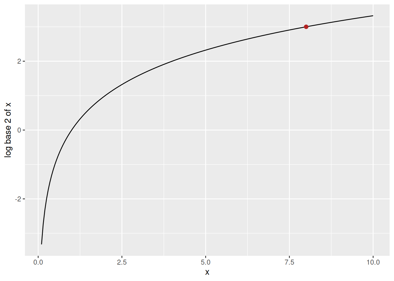
The graph of \(\log_2 x\) passes through \((8, 3)\), the first of these two facts.
Show code
x<-seq(0.1, 10, length.out =200)y<-log2(x)curve<-tibble::tibble(x =x, y =y)marked<-tibble::tibble(x =8, y =3)log_plot<-ggplot2::ggplot(curve, ggplot2::aes(x =x, y =y))+ggplot2::geom_line()+ggplot2::geom_point(data =marked, colour ="firebrick", size =2)+ggplot2::labs(x ="x", y ="log base 2 of x")log_plot
DefDefinition 29 (Real powers of zero and of negative numbers)
\((-8)^2 = 64\) and \((-8)^{-1} = -\tfrac{1}{8}\) are defined, since the exponents are integers.
\((-8)^{1/3}\) is undefined, even though \((-2)^3 = -8\). R follows the same convention: (-8)^(1/3) is NaN.
LemTheorem 2 (\(\operatorname{exp}\) and \(\operatorname{log}\) are mutual inverses)
Theorem 2 (\(\operatorname{exp}\) and \(\operatorname{log}\) are mutual inverses)
For every \(a > 0\): \({\operatorname{exp}\mathopen{}\left\{{\operatorname{log}\mathopen{}\left\{a\right\}\mathclose{}}\right\}\mathclose{}} = a\).
For every \(a \in \mathbb{R}\): \({\operatorname{log}\mathopen{}\left\{{\operatorname{exp}\mathopen{}\left\{a\right\}\mathclose{}}\right\}\mathclose{}} = a\).
RemarkRemark 5 (The logarithm to base \(b\) through the natural logarithm)
Remark 5 (The logarithm to base \(b\) through the natural logarithm). For each \(x > 0\), exactly one \(y\) satisfies Definition 28, and \[\log_b x = \frac{{\operatorname{log}\mathopen{}\left\{x\right\}\mathclose{}}}{{\operatorname{log}\mathopen{}\left\{b\right\}\mathclose{}}}.\]
To see why, note that by Definition 27, \(b^y = {\operatorname{exp}\mathopen{}\left\{y \cdot{\operatorname{log}\mathopen{}\left\{b\right\}\mathclose{}}\right\}\mathclose{}}\), so we need \({\operatorname{exp}\mathopen{}\left\{y \cdot{\operatorname{log}\mathopen{}\left\{b\right\}\mathclose{}}\right\}\mathclose{}} = x\). If \(y \cdot{\operatorname{log}\mathopen{}\left\{b\right\}\mathclose{}} = {\operatorname{log}\mathopen{}\left\{x\right\}\mathclose{}}\), then \({\operatorname{exp}\mathopen{}\left\{y \cdot{\operatorname{log}\mathopen{}\left\{b\right\}\mathclose{}}\right\}\mathclose{}} = {\operatorname{exp}\mathopen{}\left\{{\operatorname{log}\mathopen{}\left\{x\right\}\mathclose{}}\right\}\mathclose{}} = x\), by part 1 of Theorem 2. Conversely, if \({\operatorname{exp}\mathopen{}\left\{y \cdot{\operatorname{log}\mathopen{}\left\{b\right\}\mathclose{}}\right\}\mathclose{}} = x\), then applying \(\operatorname{log}\) to both sides gives \(y \cdot{\operatorname{log}\mathopen{}\left\{b\right\}\mathclose{}} = {\operatorname{log}\mathopen{}\left\{x\right\}\mathclose{}}\), by part 2 of Theorem 2. Since \(b \ne 1\), \({\operatorname{log}\mathopen{}\left\{b\right\}\mathclose{}} \ne 0\), so we can divide by it, and \(y = \frac{{\operatorname{log}\mathopen{}\left\{x\right\}\mathclose{}}}{{\operatorname{log}\mathopen{}\left\{b\right\}\mathclose{}}}\) is the only solution.
Proof. Since \(a > 0\) and \(b > 0\), the quotient \(\frac{a}{b}\) is positive, so Theorem 3 applies to the product \(\frac{a}{b} \cdot b\):
\[
\begin{aligned}
{\operatorname{log}\mathopen{}\left\{a\right\}\mathclose{}}
&= {\operatorname{log}\mathopen{}\left\{\frac{a}{b} \cdot b\right\}\mathclose{}}
&& \text{(} a = \tfrac{a}{b} \cdot b \text{)}
\\
&= {\operatorname{log}\mathopen{}\left\{\frac{a}{b}\right\}\mathclose{}} + {\operatorname{log}\mathopen{}\left\{b\right\}\mathclose{}}
&& \text{(logarithm of a product)}
\end{aligned}
\]
The second step applies Theorem 3. Subtracting \({\operatorname{log}\mathopen{}\left\{b\right\}\mathclose{}}\) from both sides gives \({\operatorname{log}\mathopen{}\left\{a\right\}\mathclose{}} - {\operatorname{log}\mathopen{}\left\{b\right\}\mathclose{}} = {\operatorname{log}\mathopen{}\left\{\frac{a}{b}\right\}\mathclose{}}\).
Example 21 (Exponential of a sum) With \(a = 2\) and \(b = 3\), \({\operatorname{exp}\mathopen{}\left\{2 + 3\right\}\mathclose{}} = {\operatorname{exp}\mathopen{}\left\{5\right\}\mathclose{}} \approx 148.41\), and \({\operatorname{exp}\mathopen{}\left\{2\right\}\mathclose{}} \cdot{\operatorname{exp}\mathopen{}\left\{3\right\}\mathclose{}} \approx 7.3891 \cdot 20.0855 \approx 148.41\).
Corollary 2 (Exponential of a difference) The exponential of a difference is the exponential of the first term divided by the exponential of the second term:
Example 22 (Exponential of a difference) With \(a = 5\) and \(b = 2\), \({\operatorname{exp}\mathopen{}\left\{5 - 2\right\}\mathclose{}} = {\operatorname{exp}\mathopen{}\left\{3\right\}\mathclose{}} \approx 20.09\), and \(\frac{{\operatorname{exp}\mathopen{}\left\{5\right\}\mathclose{}}}{{\operatorname{exp}\mathopen{}\left\{2\right\}\mathclose{}}} \approx \frac{148.4132}{7.3891} \approx 20.09\).
So \(a^{bc} \neq \mathopen{}\left(a^b\right)\mathclose{}^c\) here, which is why Theorem 9 requires \(a > 0\). The third expression, \(\mathopen{}\left(a^c\right)\mathclose{}^b = \mathopen{}\left((-1)^{\frac{1}{2}}\right)\mathclose{}^2\), is not even a real number.
RemarkRemark 7 (Tarski’s identities are not complete)
Remark 7 (Tarski’s identities are not complete). Tarski asked whether every identity in \(+\), \(\times\), exponentiation and 1 that is true for all positive integers can be derived from the eleven identities in Remark 6. It cannot: Wilkie found an identity that is true for all positive integers but does not follow from them. So this list is a useful core, not a complete rulebook.
Definition 30 (Contour line) For a function \(g\) of two real variables \(b\) and \(c\) and a number \(k\), the contour line[16] of \(g\) at height \(k\) is the set of points where \(g\) equals \(k\):
\[\mathopen{}\left\{(b, c) : g(b, c) = k\right\}\mathclose{}\]
Example 26 (Contour lines of a bowl) For \(g(b, c) = b^2 + c^2\), the contour line at height \(k = 4\) is \(\mathopen{}\left\{(b, c) : b^2 + c^2 = 4\right\}\mathclose{}\), the circle of radius \(2\) around \((0, 0)\): for example,
The contour line at height \(k = -1\) is empty, because \(b^2 + c^2 \ge 0\) for all \(b\) and \(c\).
Show code
library(ggplot2)# The bowl g(b, c) = b^2 + c^2 on a grid, and the two points of the example.bowl<-expand.grid( b =seq(-3.5, 3.5, length.out =200), c =seq(-3.5, 3.5, length.out =200))bowl$g<-bowl$b^2+bowl$c^2on_circle<-data.frame(b =c(2, 0), c =c(0, -2))contour_plot<-ggplot(bowl)+aes(b, c)+geom_contour(aes(z =g, colour =factor(after_stat(level))), breaks =c(1, 4, 9))+geom_point(data =on_circle, size =2.5)+scale_colour_viridis_d(name ="height k", end =0.85)+coord_fixed(expand =FALSE)+labs(x ="first coordinate, b", y ="second coordinate, c")+theme(legend.position ="bottom")if(knitr::is_html_output()){htmltools::div( role ="img", `aria-label` =fig_alt_contour_bowl,plotly::ggplotly(contour_plot)|>plotly::layout( legend =list(orientation ="h", x =0.5, xanchor ="center", y =-0.25))|>plotly::config(displaylogo =FALSE, responsive =TRUE))}else{contour_plot}
Figure 1: The contour lines of \(g(b, c) = b^2 + c^2\) at heights \(1\), \(4\) and \(9\). The dots mark the points \((2, 0)\) and \((0, -2)\) of the example on the circle at height \(4\).
RemarkRemark 8 (Contour lines on a plot of a surface)
Remark 8 (Contour lines on a plot of a surface). On a plot of the surface \(z = g(b, c)\), the contour line is the curve along which the surface has height \(k\).
ExrExercise 2 (Exponentiation versus multiplication)
Exercise 2 (Exponentiation versus multiplication) For \(b,c \in \mathbb{R}\), when does \(b^c = bc\)?
Solution 2. We only count a pair \((b, c)\) when \(b^c\) is defined, so for \(b < 0\) we only consider integer \(c\) (Definition 29). With that convention, \(bc = b^c\) in each of the following cases:
For \(b < 0\), cases 4 and 5 come from \(b^{c-1} = c\) as well: when \(c - 1\) is even, \(b^{c-1} > 0\), so \(c\) must be positive; when \(c - 1\) is odd, \(b^{c-1} < 0\), so \(c\) must be negative.
See the red contours in Figure 3 for a visualization of the \(b \ge 0\) cases.
Show code
mult_f<-function(b, c)b*cpow_f<-function(b, c)b^cvalues_b<-seq(0, 5, by =.01)values_c<-seq(-.5, 3, by =.01)mult_mat<-outer(values_b, values_c, mult_f)pow_mat<-outer(values_b, values_c, pow_f)pow_mat[is.infinite(pow_mat)]<-NAopacity<-.3z_min<-min(mult_mat, pow_mat, na.rm =TRUE)z_max<-5plotly::plot_ly( x =~values_b, y =~values_c)|>plotly::add_surface( z =~t(mult_mat), contours =list( z =list( show =TRUE, start =-1, end =1, size =.1)), name ="b*c", showscale =FALSE, opacity =opacity, colorscale =list(c(0, 1), c("green", "green")))|>plotly::add_surface( opacity =opacity, colorscale =list(c(0, 1), c("red", "red")), z =~t(pow_mat), contours =list( z =list( show =TRUE, start =z_min, end =z_max, size =.2)), showscale =FALSE, name ="b^c")|>plotly::layout( scene =list( xaxis =list(# type = "log", title ="First input, b"), yaxis =list(# type = "log", title ="Second input, c"), zaxis =list(# type = "log", range =c(z_min, z_max), title ="outcome"), camera =list(eye =list(x =-1.25, y =-1.25, z =0.5)), aspectratio =list(x =.9, y =.8, z =0.7)))
Figure 2: Graph of \(b*c\) and \(b^c\)
Show code
pow_minus_mult_f<-function(b, c)pow_f(b, c)-mult_f(b, c)mat1<-outer(values_b, values_c, pow_minus_mult_f)mat1[is.infinite(mat1)]<-NAopacity<-.3plotly::plot_ly( x =~values_b, y =~values_c)|>plotly::add_surface( z =~t(mat1), contours =list( z =list( show =TRUE, start =0, end =1, size =1, color ="red")), name ="b^c - b*c", showscale =TRUE, opacity =opacity)|>plotly::layout( scene =list( xaxis =list(# type = "log", title ="First input, b"), yaxis =list(# type = "log", title ="Second input, c"), zaxis =list( title ="outcome"), camera =list(eye =list(x =-1.25, y =-1.25, z =0.5)), aspectratio =list(x =.9, y =.8, z =0.7)))
Figure 3: Graph of \(b^c - b*c\). The red contour lines are at heights \(0\) and \(1\); the ones at height \(0\) show where \(b^c = b*c\).
Theorem 10 (When exponentiation equals multiplication) Let \(b, c \in \mathbb{R}\), where \(b^c\) is defined (for \(b < 0\), only integer \(c\) is allowed; Definition 29). Then \(b^c = bc\) if and only if one of the following holds:
Solution 3. Short answer: rarely (that’s all you need to know for this course).
Long answer:
Split on whether \(a > 0\) or \(a = 0\), because the logarithm we use for \(a > 0\) is undefined at \(a = 0\).
Case \(a > 0\). By Theorem 9, \((a^b)^c = a^{bc}\), so the question becomes when \(a^{bc} = a^{(b^c)}\) (for pairs \((b, c)\) where \(b^c\) is defined). Because \(a > 0\), both sides are positive, and we can take logarithms (Theorem 4):
\[
\begin{aligned}
a^{bc} &= a^{(b^c)}
\\
{\operatorname{log}\mathopen{}\left\{a^{bc}\right\}\mathclose{}} &= {\operatorname{log}\mathopen{}\left\{a^{(b^c)}\right\}\mathclose{}}
&& \text{(take logarithms of both sides)}
\\
bc \cdot {\operatorname{log}\mathopen{}\left\{a\right\}\mathclose{}} &= b^c\cdot {\operatorname{log}\mathopen{}\left\{a\right\}\mathclose{}}
&& \text{(logarithm of a power)}
\end{aligned}
\tag{2}\]
Case \(a = 0\). Here we cannot take logarithms, so we work from the values of powers of \(0\): \(0^s = 0\) for \(s > 0\) (Definition 29), \(0^0 = 1\), and \(0^s\) is undefined for \(s < 0\).
If \(b < 0\), then \(0^b\) is undefined, so \((a^b)^c\) is undefined.
If \(b > 0\), then \((0^b)^c = 0^c\) and \(b^c > 0\), so \(0^{(b^c)} = 0\); the two sides agree exactly when \(c > 0\).
LemTheorem 11 (When repeated exponentiation is not reordered)
Theorem 11 (When repeated exponentiation is not reordered) Let \(a \ge 0\) and \(b, c \in \mathbb{R}\), where \(b^c\) is defined. Then \((a^b)^c = a^{(b^c)}\), with both sides defined, if and only if
\(a > 0\) and either \(a = 1\) or \(bc = b^c\); or