\(L^p\) Spaces

Last modified: 2026-10-31 15:22:31 (PDT)

1 \(L^p\) spaces

Definition 1 (\(L^p\) norm (\(p\)-norm of a function)) Let \((S, \mathcal{S}, \mu)\) be a measure space. For any real number \(p \ge 1\), the \(L^p\) norm of a measurable function \(f : S \to \mathbb{R}\) is:

\[ \mathopen{}\left\lVert f\right\rVert\mathclose{}_p \stackrel{\text{def}}{=}\mathopen{}\left(\int_S \mathopen{}\left|f\right|\mathclose{}^p \, d\mu\right)\mathclose{}^{1/p}. \]

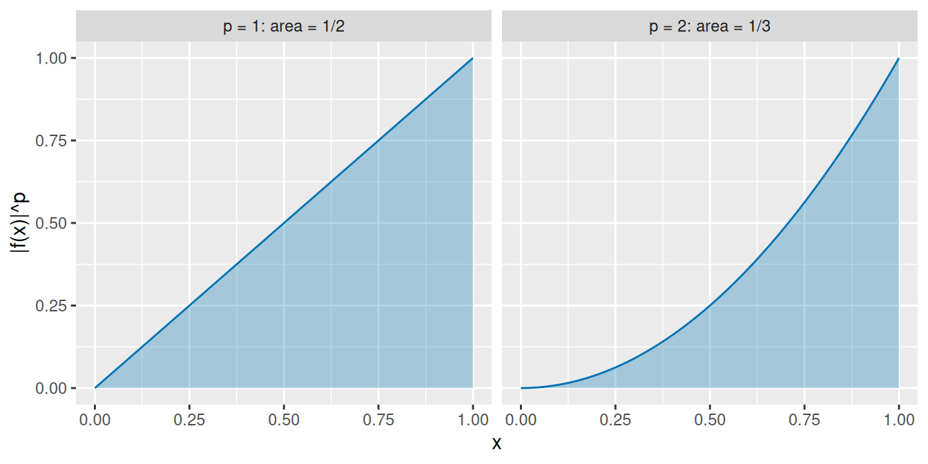
Example 1 (The \(L^1\) and \(L^2\) norms of \(x \mapsto x\) on the unit interval) Let \(S = [0, 1]\) with the Lebesgue measure \(\mu\), and let \(f(x) = x\). By Definition 1,

\[ \begin{aligned} \mathopen{}\left\lVert f\right\rVert\mathclose{}_1 &= \int_0^1 x \, dx \\ &= \frac{1}{2}, \end{aligned} \]

and

\[ \begin{aligned} \mathopen{}\left\lVert f\right\rVert\mathclose{}_2 &= \mathopen{}\left(\int_0^1 x^2 \, dx\right)\mathclose{}^{1/2} \\ &= \mathopen{}\left(\frac{1}{3}\right)\mathclose{}^{1/2}. \end{aligned} \]

[Code]
lpna_x_pf <- seq(0, 1, length.out = 201)
lpna_p1_pf <- tibble::tibble(
  x = lpna_x_pf, y = lpna_x_pf, panel = "p = 1: area = 1/2"
)
lpna_sq_pf <- lpna_x_pf^2
lpna_p2_pf <- tibble::tibble(
  x = lpna_x_pf, y = lpna_sq_pf, panel = "p = 2: area = 1/3"
)
lpna_curves_pf <- dplyr::bind_rows(lpna_p1_pf, lpna_p2_pf)
lpna_aes_pf <- ggplot2::aes(x, y)
ggplot2::ggplot(lpna_curves_pf, lpna_aes_pf) +
  ggplot2::geom_area(fill = "#0072B2", alpha = 0.3) +
  ggplot2::geom_line(colour = "#0072B2") +
  ggplot2::facet_wrap(ggplot2::vars(panel)) +
  ggplot2::labs(x = "x", y = "|f(x)|^p")
[Code]
import matplotlib.pyplot as plt
import numpy as np

lpna_x_pf = np.linspace(0, 1, 201)
fig, axes = plt.subplots(1, 2, figsize=(7, 3.5), sharey=True,
                         layout="constrained")
for ax, p, title in zip(axes, [1, 2], ["p = 1: area = 1/2", "p = 2: area = 1/3"]):
    ax.fill_between(lpna_x_pf, lpna_x_pf**p, color="#0072B2", alpha=0.3)
    ax.plot(lpna_x_pf, lpna_x_pf**p, color="#0072B2")
    ax.set_title(title)
    ax.set_xlabel("x")
axes[0].set_ylabel("|f(x)|^p")
plt.show()
Figure 1: The area under \(\mathopen{}\left|f\right|\mathclose{}^p\) for \(f(x) = x\) on \([0, 1]\) in Example 1. The area is \(\mathopen{}\left\lVert f\right\rVert\mathclose{}_p^p\): \(1/2\) for \(p = 1\) and \(1/3\) for \(p = 2\), so \(\mathopen{}\left\lVert f\right\rVert\mathclose{}_2 = \sqrt{1/3}\).

Definition 2 (\(\mathcal{L}^p\) space (\(\mathcal{L}^p(S, \mathcal{S}, \mu)\))) Let \((S, \mathcal{S}, \mu)\) be a measure space. Let \(p \ge 1\) be a real number. The \(\mathcal{L}^p\) space \(\mathcal{L}^p(S, \mathcal{S}, \mu)\) is the set of all measurable functions \(f : S \to \mathbb{R}\) whose \(L^p\) norm is less than \(\infty\): \(\mathopen{}\left\lVert f\right\rVert\mathclose{}_p < \infty\).

Example 2 (An \(L^1\) function not in \(L^2\)) Consider the interval \((0, 1)\) with the Borel \(\sigma\)-algebra (Definition 3 in Sigma-Algebras) and Lebesgue measure \(\mu\) (Definition 6 in Measures and Probability Measures). Define \(f : (0, 1) \to \mathbb{R}\) by \(f(x) = x^{-1/2}\).

  1. For \(p = 1\): \[ \begin{aligned} \mathopen{}\left\lVert f\right\rVert\mathclose{}_1 &= \int_0^1 x^{-1/2} \, dx \\ &= \mathopen{}\left[2 x^{1/2}\right]\mathclose{}_0^1 \\ &= 2 \\ &< \infty, \end{aligned} \] so \(f \in \mathcal{L}^1((0, 1), \mu)\).
  2. For \(p = 2\): \[ \begin{aligned} \mathopen{}\left|f(x)\right|\mathclose{}^2 &= \mathopen{}\left(x^{-1/2}\right)\mathclose{}^2 \\ &= \frac{1}{x}. \end{aligned} \] The integral is: \[ \begin{aligned} \int_0^1 \frac{1}{x} \, dx &= \lim_{\varepsilon\to 0^+} \mathopen{}\left[\ln x\right]\mathclose{}_\varepsilon^1 \\ &= \lim_{\varepsilon\to 0^+} (-\ln \varepsilon) \\ &= \infty. \end{aligned} \] So \(\mathopen{}\left\lVert f\right\rVert\mathclose{}_2 = \infty\), so \(f \notin \mathcal{L}^2((0, 1), \mu)\).

This shows that \(\mathcal{L}^2 \subset \mathcal{L}^1\) on sets of finite measure: a larger \(p\) imposes stricter requirements near singularities.

[Code]
lpss_x_pf <- seq(0.01, 1, length.out = 400)
lpss_root_pf <- lpss_x_pf^(-1 / 2)
lpss_p1_pf <- tibble::tibble(
  x = lpss_x_pf, y = lpss_root_pf, panel = "p = 1: area = 2"
)
lpss_inv_pf <- 1 / lpss_x_pf
lpss_p2_pf <- tibble::tibble(
  x = lpss_x_pf, y = lpss_inv_pf, panel = "p = 2: area = infinity"
)
lpss_curves_pf <- dplyr::bind_rows(lpss_p1_pf, lpss_p2_pf)
lpss_aes_pf <- ggplot2::aes(x, y, fill = panel, colour = panel)
lpss_colours_pf <- c("#0072B2", "#D55E00")
lpss_ylim_pf <- c(0, 10)
ggplot2::ggplot(lpss_curves_pf, lpss_aes_pf) +
  ggplot2::geom_area(alpha = 0.3, colour = NA) +
  ggplot2::geom_line() +
  ggplot2::facet_wrap(ggplot2::vars(panel)) +
  ggplot2::scale_fill_manual(values = lpss_colours_pf) +
  ggplot2::scale_colour_manual(values = lpss_colours_pf) +
  ggplot2::coord_cartesian(ylim = lpss_ylim_pf) +
  ggplot2::guides(fill = "none", colour = "none") +
  ggplot2::labs(x = "x", y = "|f(x)|^p")
[Code]
import matplotlib.pyplot as plt
import numpy as np

lpss_x_pf = np.linspace(0.01, 1, 400)
lpss_curves_pf = [
    ("p = 1: area = 2", lpss_x_pf ** (-1 / 2), "#0072B2"),
    ("p = 2: area = infinity", 1 / lpss_x_pf, "#D55E00"),
]
fig, axes = plt.subplots(1, 2, figsize=(7, 3.5), sharey=True,
                         layout="constrained")
for ax, (title, y, colour) in zip(axes, lpss_curves_pf):
    ax.fill_between(lpss_x_pf, y, color=colour, alpha=0.3)
    ax.plot(lpss_x_pf, y, color=colour)
    ax.set_title(title)
    ax.set_xlabel("x")
    ax.set_ylim(0, 10)
#> <matplotlib.collections.FillBetweenPolyCollection object at 0x7f5dc77c2490>
#> [<matplotlib.lines.Line2D object at 0x7f5dc77c25d0>]
#> Text(0.5, 1.0, 'p = 1: area = 2')
#> Text(0.5, 0, 'x')
#> (0.0, 10.0)
#> <matplotlib.collections.FillBetweenPolyCollection object at 0x7f5dc77c2710>
#> [<matplotlib.lines.Line2D object at 0x7f5dc77c2850>]
#> Text(0.5, 1.0, 'p = 2: area = infinity')
#> Text(0.5, 0, 'x')
#> (0.0, 10.0)
axes[0].set_ylabel("|f(x)|^p")
plt.show()
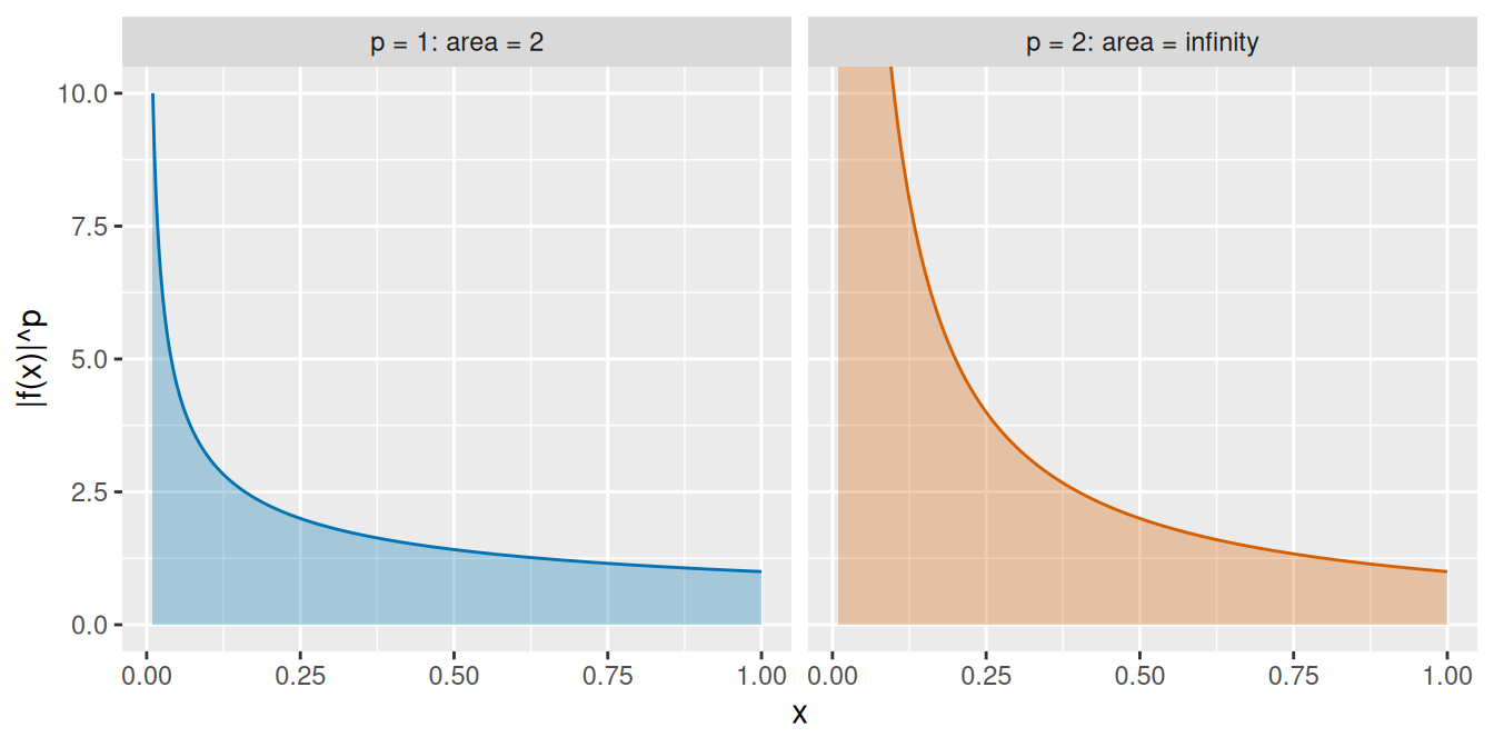
Figure 2: The area under \(\mathopen{}\left|f\right|\mathclose{}^p\) for \(f(x) = x^{-1/2}\) on \((0, 1)\) in Example 2. The curve for \(p = 1\) has area \(2\), so \(f \in \mathcal{L}^1\). The curve for \(p = 2\) keeps climbing toward \(x = 0\) and its area is \(\infty\), so \(f \notin \mathcal{L}^2\). The plots cut the curves off at \(10\).

Definition 3 (Equal almost everywhere (\(f = g\) \(\mu\)-a.e.)) Let \((S, \mathcal{S}, \mu)\) be a measure space. Let \(f, g : S \to \mathbb{R}\) be measurable. The functions \(f\) and \(g\) are equal almost everywhere, written \(f = g\) \(\mu\)-a.e., if \(f(s) = g(s)\) holds almost everywhere.

Example 3 (A function that differs from \(0\) at one point) Let \(S = \mathbb{R}\) with the Lebesgue measure \(\mu\). Let \(f(s) = 1\) if \(s = 0\), and \(f(s) = 0\) otherwise. The set \({\mathopen{}\left\{s : f(s) \neq 0\right\}\mathclose{}} = {\mathopen{}\left\{0\right\}\mathclose{}}\) has measure zero, so \(f = 0\) almost everywhere by Definition 3.

Definition 4 (\(L^p\) space (\(L^p(S, \mathcal{S}, \mu)\), \(L^p(\mu)\))) Let \((S, \mathcal{S}, \mu)\) be a measure space. Let \(p \ge 1\) be a real number. For each \(f\) in the \(\mathcal{L}^p\) space, let \([f]\) be the set of all functions in \(\mathcal{L}^p(S, \mathcal{S}, \mu)\) that are equal almost everywhere to \(f\). The \(L^p\) space \(L^p(S, \mathcal{S}, \mu)\) (or simply \(L^p(\mu)\)) is the set of all such sets \([f]\), with the norm \(\mathopen{}\left\lVert[f]\right\rVert\mathclose{}_p \stackrel{\text{def}}{=}\mathopen{}\left\lVert f\right\rVert\mathclose{}_p\) (\(L^p\) norm).

Example 4 (The zero element of \(L^p\)) Let \(f\) be the function in Example 3, which is \(1\) at \(s = 0\) and \(0\) elsewhere. Then \(f = 0\) almost everywhere, so \([f] = [0]\). Also \(\mathopen{}\left\lVert f\right\rVert\mathclose{}_p = 0\) although \(f \neq 0\), so \(\mathopen{}\left\lVert f\right\rVert\mathclose{}_p = 0\) can hold for a nonzero element of \(\mathcal{L}^p\); on \(L^p(\mu)\), \(\mathopen{}\left\lVert[f]\right\rVert\mathclose{}_p = 0\) only for \([f] = [0]\), as a norm requires.

Definition 5 (Essential supremum norm (\(L^\infty\) norm)) Let \((S, \mathcal{S}, \mu)\) be a measure space. The essential supremum norm (or \(L^\infty\) norm) of a measurable function \(f : S \to \mathbb{R}\) is:

\[ \mathopen{}\left\lVert f\right\rVert\mathclose{}_\infty \stackrel{\text{def}}{=}\inf \mathopen{}\left\{ C \ge 0 : \mu(\mathopen{}\left\{s \in S : \mathopen{}\left|f(s)\right|\mathclose{} > C\right\}\mathclose{}) = 0 \right\}\mathclose{}. \]

Example 5 (The essential supremum norm ignores a null set) Let \(S = [0, 1]\) with the Lebesgue measure \(\mu\). Let \(f(s) = 5\) if \(s = 0\) and \(f(s) = s\) otherwise. Then \(\sup_s \mathopen{}\left|f(s)\right|\mathclose{} = 5\). For \(C \ge 1\), the set \({\mathopen{}\left\{s : \mathopen{}\left|f(s)\right|\mathclose{} > C\right\}\mathclose{}}\) is empty or \({\mathopen{}\left\{0\right\}\mathclose{}}\), so it has measure zero, and for \(C < 1\) it has positive measure. By Definition 5, \(\mathopen{}\left\lVert f\right\rVert\mathclose{}_\infty = 1\).

[Code]
esn_x_pf <- seq(0, 1, length.out = 101)
esn_line_pf <- tibble::tibble(x = esn_x_pf, y = esn_x_pf)
esn_open_pf <- tibble::tibble(x = 0, y = 0)
esn_spike_pf <- tibble::tibble(x = 0, y = 5)
esn_aes_pf <- ggplot2::aes(x, y)
ggplot2::ggplot(esn_line_pf, esn_aes_pf) +
  ggplot2::geom_line(colour = "#0072B2") +
  ggplot2::geom_point(data = esn_open_pf, shape = 1, size = 3) +
  ggplot2::geom_point(data = esn_spike_pf, colour = "#D55E00", size = 3) +
  ggplot2::geom_hline(yintercept = 1, linetype = "dashed") +
  ggplot2::labs(x = "s", y = "f(s)")
[Code]
import matplotlib.pyplot as plt
import numpy as np

esn_x_pf = np.linspace(0, 1, 101)
fig, ax = plt.subplots(figsize=(5, 3.5), layout="constrained")
ax.plot(esn_x_pf, esn_x_pf, color="#0072B2")
ax.plot(0, 0, marker="o", markerfacecolor="white", color="black")
ax.plot(0, 5, marker="o", color="#D55E00")
ax.axhline(1, linestyle="dashed", color="black")
ax.set_xlabel("s")
ax.set_ylabel("f(s)")
plt.show()
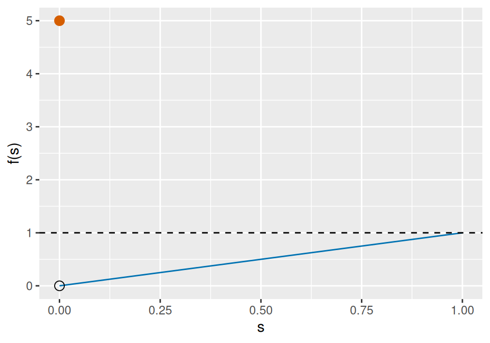
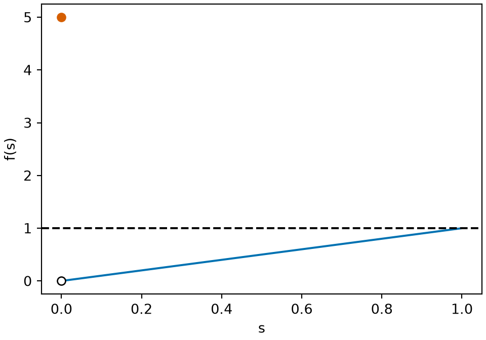
Figure 3: The function in Example 5: \(f(s) = s\) except \(f(0) = 5\). The supremum is \(5\), reached only at the single point \(s = 0\), which has measure zero, so the essential supremum norm is the dashed height \(1\).

Definition 6 (\(\mathcal{L}^\infty\) space (\(\mathcal{L}^\infty(S, \mathcal{S}, \mu)\))) Let \((S, \mathcal{S}, \mu)\) be a measure space. The \(\mathcal{L}^\infty\) space \(\mathcal{L}^\infty(S, \mathcal{S}, \mu)\) is the set of all measurable functions \(f : S \to \mathbb{R}\) whose essential supremum norm is less than \(\infty\): \(\mathopen{}\left\lVert f\right\rVert\mathclose{}_\infty < \infty\).

Example 6 (Bounded and unbounded functions) Let \(S = (0, 1)\) with the Lebesgue measure \(\mu\). The function \(f(s) = s\) has \(\mathopen{}\left\lVert f\right\rVert\mathclose{}_\infty = 1 < \infty\), so \(f \in \mathcal{L}^\infty(S, \mathcal{S}, \mu)\) by Definition 6. The function \(g(s) = 1/s\) exceeds every \(C\) on the set \((0, 1/C)\) of positive measure, so \(\mathopen{}\left\lVert g\right\rVert\mathclose{}_\infty = \infty\) and \(g \notin \mathcal{L}^\infty(S, \mathcal{S}, \mu)\).

Definition 7 (\(L^\infty\) space (\(L^\infty(S, \mathcal{S}, \mu)\), \(L^\infty(\mu)\))) Let \((S, \mathcal{S}, \mu)\) be a measure space. For each \(f\) in the \(\mathcal{L}^\infty\) space, let \([f]\) be the set of all functions in \(\mathcal{L}^\infty(S, \mathcal{S}, \mu)\) that are equal almost everywhere to \(f\). The \(L^\infty\) space \(L^\infty(S, \mathcal{S}, \mu)\) (or simply \(L^\infty(\mu)\)) is the set of all such sets \([f]\), with the norm \(\mathopen{}\left\lVert[f]\right\rVert\mathclose{}_\infty \stackrel{\text{def}}{=}\mathopen{}\left\lVert f\right\rVert\mathclose{}_\infty\) (essential supremum norm).

Example 7 (Bounded functions equal almost everywhere) Let \(f\) be the function in Example 5 and \(h(s) = s\) on \([0, 1]\). Then \(f = h\) almost everywhere (Definition 3), so \([f] = [h]\) in \(L^\infty(\mu)\), and \(\mathopen{}\left\lVert[f]\right\rVert\mathclose{}_\infty = \mathopen{}\left\lVert h\right\rVert\mathclose{}_\infty = 1\).

Theorem 1 (Holder’s inequality) Let \((S, \mathcal{S}, \mu)\) be a measure space, and let \(p, q \in [1, \infty]\) be conjugate exponents satisfying \(\frac{1}{p} + \frac{1}{q} = 1\) (with the convention that \(q = \infty\) when \(p = 1\), and \(q = 1\) when \(p = \infty\)). If \(f \in L^p(\mu)\) and \(g \in L^q(\mu)\) (Definition 4), then their product \(f g\) is absolutely integrable (\(f g \in L^1(\mu)\)) and satisfies:

\[ \mathopen{}\left\lVert f g\right\rVert\mathclose{}_1 = \int_S \mathopen{}\left|f g\right|\mathclose{} \, d\mu\le \mathopen{}\left\lVert f\right\rVert\mathclose{}_p\,\mathopen{}\left\lVert g\right\rVert\mathclose{}_q. \]

When

\[ \begin{aligned} p &= q \\ &= 2, \end{aligned} \]

this inequality is the Cauchy-Schwarz inequality for integrals.

Theorem 2 (Minkowski’s inequality (\(L^p\) triangle inequality)) Let \((S, \mathcal{S}, \mu)\) be a measure space and let \(1 \le p \le \infty\). For any functions \(f, g \in L^p(\mu)\) (Definition 4), their sum \(f + g\) is in \(L^p(\mu)\) and satisfies:

\[ \mathopen{}\left\lVert f + g\right\rVert\mathclose{}_p \le \mathopen{}\left\lVert f\right\rVert\mathclose{}_p + \mathopen{}\left\lVert g\right\rVert\mathclose{}_p. \]

Together with absolute homogeneity \(\mathopen{}\left\lVert c f\right\rVert\mathclose{}_p = \mathopen{}\left|c\right|\mathclose{}\,\mathopen{}\left\lVert f\right\rVert\mathclose{}_p\) and definiteness, Minkowski’s inequality establishes that \(L^p(\mu)\) satisfies all axioms of a normed vector space.

Example 8 (Applying Holder’s inequality to finite sums and expectations)  

  1. Finite vectors (Cauchy-Schwarz and taxicab bounds): Equipping a finite set with the counting measure, Holder’s inequality for conjugate exponents \(p, q\) gives: \[ \sum_{i=1}^n\mathopen{}\left|x_i y_i\right|\mathclose{} \le \mathopen{}\left(\sum_{i=1}^n\mathopen{}\left|x_i\right|\mathclose{}^p\right)\mathclose{}^{1/p} \mathopen{}\left(\sum_{i=1}^n\mathopen{}\left|y_i\right|\mathclose{}^q\right)\mathclose{}^{1/q}. \] Setting \(p = 1\), \(q = \infty\) gives \(\sum_{i=1}^n\mathopen{}\left|x_i y_i\right|\mathclose{} \le \mathopen{}\left\lVert\mathord{\smash[b]{\underset{\raise.3ex\hbox{$\scriptstyle\sim$}}{x}}\vphantom{x}}\right\rVert\mathclose{}_1\,\mathopen{}\left\lVert\mathord{\smash[b]{\underset{\raise.3ex\hbox{$\scriptstyle\sim$}}{y}}\vphantom{y}}\right\rVert\mathclose{}_\infty\). Setting

    \[ \begin{aligned} p &= q \\ &= 2 \end{aligned} \]

    gives the standard vector Cauchy-Schwarz inequality.

  2. Covariance bound for random variables: On a probability space with measure \(\mathbb{P}\) (Definition 12 in Measures and Probability Measures), taking

    \[ \begin{aligned} p &= q \\ &= 2 \end{aligned} \]

    gives \({\mathbb{E}\mathopen{}\left[\mathopen{}\left|X Y\right|\mathclose{}\right]\mathclose{}} \le \sqrt{{\mathbb{E}\mathopen{}\left[X^2\right]\mathclose{}}}\,\sqrt{{\mathbb{E}\mathopen{}\left[Y^2\right]\mathclose{}}}\), guaranteeing that the covariance between any two square-integrable random variables is finite.

Remark 1 (\(L^p\) spaces and norms in probability and machine learning). In probability, statistics, and machine learning, \(L^p\) spaces structure the geometry of random variables, estimators, and loss functions:

  1. Random variables, moments, and inclusion of \(L^p\) spaces: When \(\mu= \mathbb{P}\) is a probability measure (Definition 12 in Measures and Probability Measures) with total measure \({\mathbb{P}\mathopen{}\left(S\right)\mathclose{}} = 1\), an \(L^p\) function is a random variable \(X\) with finite \(p\)-th moment: \[ \mathopen{}\left\lVert X\right\rVert\mathclose{}_p = \mathopen{}\left({\mathbb{E}\mathopen{}\left[\mathopen{}\left|X\right|\mathclose{}^p\right]\mathclose{}}\right)\mathclose{}^{1/p}. \] By Jensen’s inequality, if \(1 \le p \le q \le \infty\), then \(\mathopen{}\left\lVert X\right\rVert\mathclose{}_p \le \mathopen{}\left\lVert X\right\rVert\mathclose{}_q\), so \(L^q(P) \subseteq L^p(P)\). For instance, every random variable with finite variance (\(X \in L^2\)) has finite expectation (\(X \in L^1\)).

  2. The unique Hilbert space \(L^2\) and conditional expectation: Among all \(L^p\) spaces, only \(L^2(\mu)\) is an inner product space, equipped with the inner product \({\mathopen{}\left\langle f, g\right\rangle\mathclose{}} \stackrel{\text{def}}{=}\int_S f g \, d\mu\) (all other \(L^p\) spaces fail the parallelogram law). The completeness of \(L^2\) makes it a Hilbert space. In regression, the conditional expectation \({\mathbb{E}\mathopen{}\left[Y \mid X\right]\mathclose{}}\) is the orthogonal projection of \(Y \in L^2\) onto the closed subspace of \(L^2\) functions measurable with respect to \(X\), minimizing the population mean squared error (pMSE) \(\mathopen{}\left\lVert Y - g(X)\right\rVert\mathclose{}_2^2\).

  3. Loss functions, estimation, and robustness: The choice of \(p\) in \(L^p\) norms defines loss functions for optimization and regression:

    • \(L^2\) loss (population mean squared error (pMSE), or sample mean squared error (sMSE) on a sample): penalizes large errors quadratically, yielding the conditional mean; sensitive to outliers.
    • \(L^1\) loss (population mean absolute error (pMAE), or sample mean absolute error (sMAE) on a sample): penalizes errors linearly, yielding the conditional median; robust to heavy tails and outliers.
    • \(L^\infty\) loss (Chebyshev criterion): minimizes the worst-case maximum error across all instances.