Machine Learning Experimentation
Last modified: 2026-10-28
Source
We adapted these notes from Brian Hutchinson’s Fall 2025 lecture notes, and drew on Logan Sizemore’s Spring 2025 lecture on machine-learning experimentation. That lecture covers chartjunk but not the data-ink ratio. The data-ink ratio comes from Tufte, cited in place. The sampling-bias and data-snooping sections paraphrase principles in Learning From Data [1, Ch. 5]; its example is new.
1 Why a chapter on process
Most of this course is about models: what classes of function we are willing to consider, what algorithms fit them to data, and what can be proved about how well the result will generalize. That part of machine learning has theorems, and it transfers between problems.
None of it is useful in isolation. A model is a component of something larger — a decision someone makes, a measurement someone takes, a person who acts differently than they would have — and the component can be flawless while the larger thing fails. The failure is usually not in the fitting. It lies in what we fit, what data we fit it to, how we measure it, and what we compare it against.
This chapter is about that surrounding work: conducting a machine learning experiment from start to finish.
Exercise 1 (A good model and a failed project)
Exercise 1 (A good model and a failed project) A team trains a classifier that reaches 99.4% accuracy on data it was never fitted to. Six months after the team deploys the system, the project is cancelled.
Name three distinct ways this can happen without the model ever having been wrong about the question it was actually asked.
Solution 1. Three, and no two of them occur at the same place in the process.
The metric was not the objective. If 99.4% of the cases are negative, the constant predictor “never” also scores 99.4%, and the model may be doing exactly that. Accuracy on an imbalanced problem can be high while the quantity anyone cares about — how many of the rare positives were caught — is zero. Choosing what to measure is its own step, and it comes before training.
The data did not match deployment. The model was fitted to a sample that deployment does not resemble: a different population, a different time, a different instrument. The sharpest version of this is target leakage, where a feature encodes the label through a route that will not exist at prediction time — a record written only for cases that were later confirmed, a timestamp that differs systematically between classes. Held-out accuracy is high because the held-out data carries the same feature. This is a different failure from test-set leakage, the contamination of the training split by held-out records, which Splitting the data covers later; they share a word and nothing else. Target leakage survives a perfectly clean split.
The prediction changed no decision. The output arrives too late to act on, or costs more per case than the error it prevents, or reaches someone who has no authority to do anything differently. The model answers a question correctly and nobody was going to change any action based on the answer.
Each of the three is invisible to the training loss and to the held-out score. No amount of better fitting finds any of them.
2 One blueprint
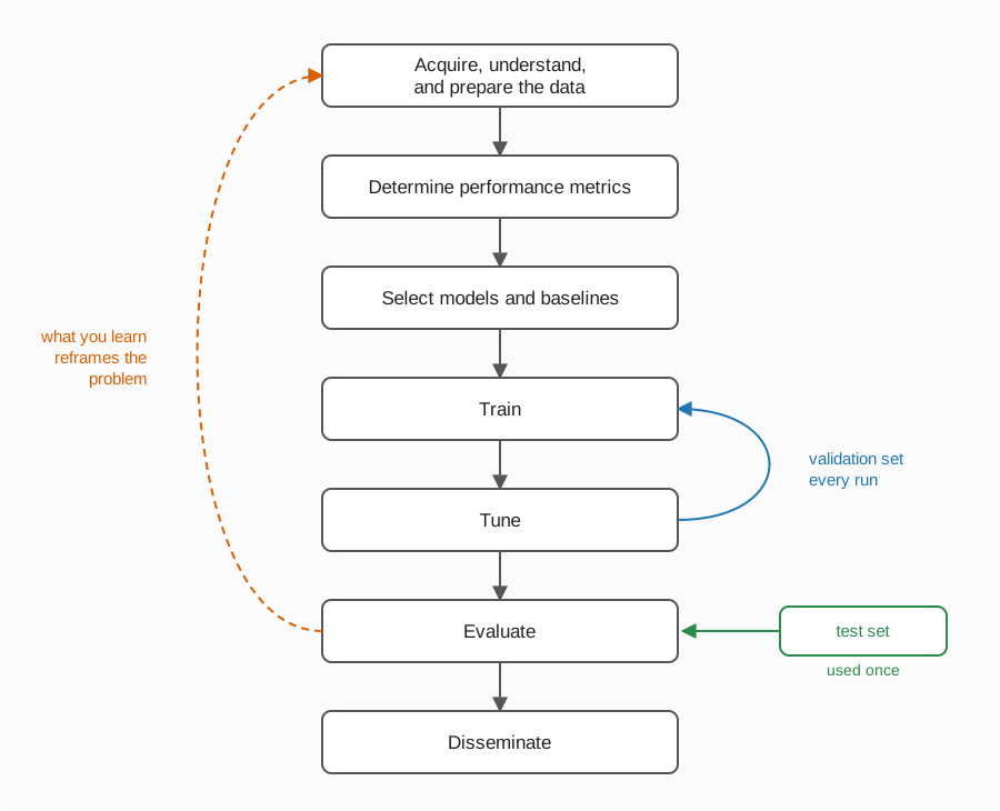
Figure 1 is one blueprint. It is not comprehensive and it cannot be: machine learning work spans enough problems, data types and deployment settings that any single ordering of the steps is wrong somewhere. A reinforcement-learning agent gathers its own data as it runs, so “acquire the data” is not a stage that finishes. An online system retrains continuously, so “evaluate” is a monitor rather than a milestone.
Treat it as a default to depart from deliberately. Having a default at all makes a departure visible as a departure.
The three failures of Exercise 1 fit the chart unevenly. Two have a box: the wrong metric belongs to the metric-setting step, and the unrepresentative sample belongs to the data step. The third has none. A prediction nobody acts on fails past the last box altogether, where the deployed system operates and where the chart stops drawing.
Exercise 2 (What each stage consumes and emits)
Exercise 2 (What each stage consumes and emits) Work down the column of Figure 1. For each of the seven boxes, name what it takes in and what it passes on.
Two are filled in. Do the other five.
| Stage | Consumes | Emits |
|---|---|---|
| Acquire, understand, prepare | a question, and whatever raw data exists | train / validation / test splits |
| Determine performance metrics | ||
| Select models and baselines | ||
| Train | ||
| Tune | ||
| Evaluate | ||
| Disseminate | a test-set number and the analyses behind it | a claim someone else can act on |
Solution 2.
| Stage | Consumes | Emits |
|---|---|---|
| Acquire, understand, prepare | a question, and whatever raw data exists | train / validation / test splits |
| Determine performance metrics | the question, and what the decision costs | a scoring rule, fixed in advance |
| Select models and baselines | the data’s shape and size, and the metric | a shortlist of model families, and at least one baseline |
| Train | the training split, one family off the shortlist, and one setting of its hyperparameters | a fitted model |
| Tune | a fitted model, the validation split, and the scoring rule | the next setting to try, or the best model found |
| Evaluate | the best model, and the test split | one number, and the analyses that explain it |
| Disseminate | a test-set number and the analyses behind it | a claim someone else can act on |
The completed table shows three things.
The metric is chosen before any model is. It is an input to model selection, not a summary of it. Deciding what counts as good after seeing which models did well is hypothesizing after the results are known (HARKing), and it removes the metric’s ability to rule anything out.
Train and tune consume different splits. Training reads the training split; tuning reads the validation split, through the scores computed on it. So they are two boxes and not one.
Each split is consumed in exactly one row, which makes the three-way division useful: train, tune and evaluate never see the same data. The test split appears once, in “evaluate”.
Train and tune may be repeated as often as the budget allows, since between them they only ever touch the training and validation splits. The first three rows may be revisited too — but that is a repetition of the outer loop, taken deliberately and written down, not a quiet re-decision made because a score came back disappointing.
Read
GeeksforGeeks explains the machine learning lifecycle [3].
3 The two loops
The column in Figure 1 is the easy part. The two arrows that go back up it are where the judgement is needed, and they are not the same kind of arrow.
Definition 1 (Inner loop)
Definition 1 (Inner loop) The inner loop, in blue, runs between training and tuning. Fit a model, score it on the validation set, change a hyperparameter, fit again. It runs tens or thousands of times, it is cheap enough to automate, and it never changes the question you are asking — only the settings you ask that question under.
Example 1 (Inner loop: a ridge penalty)
Example 1 (Inner loop: a ridge penalty) Fit ridge regression at \(\regpar \in \{0.01, 0.1, 1, 10, 100\}\), score each fit on the validation set, keep the best. Five fits, a few seconds, one line of code. The target, the features, the split and the metric are the same at the end as at the start — only \(\regpar\) moved.
Definition 2 (Outer loop)
Definition 2 (Outer loop) The outer loop, in orange and dashed, runs from evaluation all the way back to the data. It is needed when something you learn shows the problem was framed wrong: the labels mean something other than you assumed, the metric rewards a behaviour nobody wants, the classes you split into are not the classes that matter. It is expensive, it is rare, and repeating it invalidates everything downstream of the change.
Example 2 (Outer loop: the metric was the wrong question)
Example 2 (Outer loop: the metric was the wrong question) A fraud classifier reaches \(99\%\) accuracy on the validation set. It reaches it by predicting not fraud for every transaction, because \(1\%\) of transactions are fraud. No setting of any hyperparameter fixes this: the inner loop is optimising a number that rewards the useless model. Going back means choosing a different metric — say recall at a fixed false-positive rate — and every score computed before that change now answers a question nobody was asking.
The chart draws the outer loop as an arrow leaving evaluation, because that is where the evidence usually appears. The same loop applies to news from outside — a client naming a cost, a second dataset disagreeing with the first — and costs the same to repeat.
The dashes show the difference. The blue loop is part of the method. The orange loop shows that the method had the wrong goal, and the only thing worse than repeating it is not noticing that you should.
Exercise 3 (Which loop, or neither)
Exercise 3 (Which loop, or neither) Is the following a repetition of the inner loop (Definition 1), a repetition of the outer loop (Definition 2), or neither — and why?
Raising the regularization strength from \(0.01\) to \(0.1\) because the validation-set error went up while the training error went down.
Solution 3. Inner loop. The standard case of it: a validation-set score moved, a hyperparameter changes in response, the question is untouched. The diagnosis is the standard one — training error falling while validation error rises is overfitting, and more regularization is the response.
Exercise 4 (Which loop, or neither (part 2))
Exercise 4 (Which loop, or neither (part 2)) Use the setup of Exercise 3.
Is discovering that half the records labelled negative were never examined at all, and are unlabelled rather than negative, a repetition of the inner loop, a repetition of the outer loop, or neither, and why?
Solution 4. Outer loop. The label is not what the pipeline assumed, so every split, every metric and every score computed so far was computed on a mislabelled target. Nothing downstream survives: the fix is to go back to the data and either obtain the missing labels or restate the problem as one with a positive and an unknown class rather than two known ones.
Exercise 5 (Which loop, or neither (part 3))
Exercise 5 (Which loop, or neither (part 3)) Use the setup of Exercise 3.
Is refitting the winning configuration five times under different random seeds, and reporting the spread of its validation-set scores, a repetition of the inner loop, a repetition of the outer loop, or neither, and why?
Solution 5. Neither. No hyperparameter moves and no question changes, so neither loop was repeated. The five runs measure how much of the inner loop’s ranking is noise. If the spread across seeds is wider than the gap between the top two configurations, then the inner loop did not choose between them — the seed did, and the tuning result should be reported as a tie. This check is cheap, almost everyone skips it, and it separates a ranking from a coincidence.
Exercise 6 (Which loop, or neither (part 4))
Exercise 6 (Which loop, or neither (part 4)) Use the setup of Exercise 3.
Is switching from accuracy to recall at a fixed false-positive rate, after the client says a missed case costs a hundred times a false alarm, a repetition of the inner loop, a repetition of the outer loop, or neither, and why?
Solution 6. Outer loop. The metric feeds model selection, so changing it shows the shortlist was chosen against the wrong criterion and has to be chosen again — along with everything after it. The trigger came from outside rather than from evaluation, which is the case Definition 2 names and Figure 1 does not draw. This is also the cheapest version of the loop available: the cost occurred before a number was published.
4 Use the test set only once
The green box in Figure 1 enters the chart once, at one place, with one arrow. That arrow constrains the procedure, which is the single easiest thing on the chart to get wrong.
A test-set score estimates how the chosen model will do on data drawn the way the test set was drawn. It is an honest estimate exactly as long as we make the choice without reference to it. The moment a test-set number influences a decision — which model to keep, which hyperparameter to use, whether to train a bit longer — the test set has become a second validation set, and the number it produces is a best-of-\(k\), which estimates nothing. Nothing announces this. The number still prints.
Use the test set once
Use the test set once, at the end, to report. Do not use it again to choose.
The practical form of the rule is a budget rather than a prohibition: decide in advance how many times we will read the test set, which for most of this course is once, and disclose a second reading as a result in its own right, carrying the first reading alongside it.
Exercise 7 (Four procedures)
Exercise 7 (Four procedures) Does each of the following procedures use up the test set, in the sense that the number it ends up reporting is no longer an estimate of generalization?
Train twenty models, pick the one with the best validation-set score, report its test-set score.
Solution 7. Fine. This is the procedure the chart describes. Twenty choices were made, all of them against validation-set scores; the test set saw one model, once, after the choosing was over.
Exercise 8 (Four procedures (part 2))
Exercise 8 (Four procedures (part 2)) Use the setup of Exercise 7.
Train twenty models, report the best of their twenty test-set scores. Does this procedure use up the test set?
Solution 8. Used up. The best of twenty test-set scores is the maximum of twenty noisy measurements, and a maximum is biased upward by an amount that grows with how many you took. If each score is off by a standard deviation \(\sdpar\), the expected maximum of twenty sits about \(1.87\sdpar\) above the truth; of three, about \(0.85\sdpar\). So the reported number overstates how well the model it names will do. It is also not a reliable answer to “which of the twenty is best”: the winner is whichever combined good performance with a lucky test split, and those two are not separable from one score apiece.
Exercise 9 (Four procedures (part 3))
Exercise 9 (Four procedures (part 3)) Use the setup of Exercise 7.
Report a test-set score. It is worse than the validation-set score, so train three more models and report the best of those on test. Does this procedure use up the test set?
Solution 9. Used up, and easier to miss than the procedure of Exercise 8. The bias here is the smaller of the two — a maximum over three or four scores, not twenty — so if the reported number were the only thing at stake this would be the smaller problem. Worse, the test set has now entered the design loop. The score was read, it was disappointing, and that reading caused three more models to exist. Every later number is conditioned on the first one, and nothing in the write-up records that. Géron’s checklist states the rule as a warning in exactly this place: “Don’t tweak your model after measuring the generalization error: you would just start overfitting the test set” [4], Appendix B.
Exercise 10 (Four procedures (part 4))
Exercise 10 (Four procedures (part 4)) Use the setup of Exercise 7.
Report a test-set score. While writing it up, discover the data loader dropped every record with a missing field, which is 8% of the data and not missing at random. Fix it, retrain everything, report a new test-set score. Does this procedure use up the test set?
Solution 10. Arguable, and worth arguing about. Start with what the defect did to the data. The loader dropped 8% of records, not at random, from every split — so the test set was corrupted too, and the first number was never an estimate of generalization to begin with. There is nothing there to use up, and the second reading is the first valid one.
That settles the arithmetic and leaves the conduct question. A defect in the data triggered the revision, not the size of the number, so it selected among no models: everything was retrained and there was nothing to choose between. To check that claim, ask how someone found the defect. A data audit, a failing unit test, a colleague’s question or a second dataset showing the same gap are all routes that do not run through the score. If instead the only thing that prompted the look was the disappointing number, then the score selected the fix, and this procedure is the procedure of Exercise 9 in a different form.
That question has a checkable answer, and it belongs in the write-up alongside both numbers.
Definition 3 (Data snooping)
Example 3 (Steps that snoop without anyone noticing)
Example 3 (Steps that snoop without anyone noticing) These steps look harmless:
- scaling every column by its mean and standard deviation before splitting
- choosing a transformation after plotting all the data
- keeping the features that correlate best with the label
- picking a model family because a colleague’s paper reported it worked on this benchmark
Each uses the data to decide something, and the decision goes into the model. By Definition 3, each one snoops, although none of them computes a test score.
Remark 1 (Snooping is about information, not the score)
Remark 1 (Snooping is about information, not the score). Reading the test-set score twice is the most visible way to break the rule above, but it is not the only way. The rule is about information, not about the number: the test set stops being an honest judge as soon as anything it contains has influenced a choice, in any step, including steps that never compute a test score.
Remark 2 (Two remedies for data snooping)
Remark 2 (Two remedies for data snooping). The strict remedy is discipline: put the test set away before any step that could use it, and put every data-dependent step, from scaling to feature selection, inside the training data.
The other remedy is accounting. When the data has been used, the more choices it informed, the less its score is worth, and the honest report says how many were tried. This includes choices other people made on the same benchmark. Repeated use of one data set, by one person or a whole community, behaves like a larger search over models, and searches find chance fits.
Source: Abu-Mostafa et al. [1, Ch. 5] and Abu-Mostafa [7], Lecture 17.
Exercise 11 (Select, then split)
Exercise 11 (Select, then split) A study has 40 patients, 1000 measured features per patient, and a label that is a coin flip, independent of every feature. Two analysts each try to predict the label from the 20 features that agree best with it. Analyst A picks those 20 features using all 40 patients, then splits the patients in half, fits on the first half and reports accuracy on the second. Analyst B splits first, picks the 20 features using only the first half, and reports accuracy on the second half. Which analyst’s accuracy will be higher? Predict both accuracies before you read the solution.
Solution 11. Simulate the study 200 times, with fresh random features and labels each time. Each analyst scores a patient by summing the 20 chosen features, each multiplied by the sign of its agreement with the label.
import numpy as np

# Fix the seed so that the page prints the same numbers each time it is built.
rng = np.random.default_rng(571)
n_patients, n_features, n_kept, n_studies = 40, 1000, 20, 200
accuracy_ss = {"A": [], "B": []}

for _ in range(n_studies):
    # Pure noise: the label is independent of every feature, so any
    # accuracy above 0.5 on the second half must be an artefact.
    X = rng.standard_normal((n_patients, n_features))
    y = rng.choice([-1, 1], n_patients)
    first_half = np.arange(n_patients) < n_patients // 2
    second_half = ~first_half

    # A selects on every patient, including the ones in the second half.
    # B selects on the first half only.
    for analyst, rows in (("A", np.ones(n_patients, dtype=bool)), ("B", first_half)):
        agreement = (X[rows] * y[rows, None]).mean(axis=0)
        kept = np.argsort(-np.abs(agreement))[:n_kept]
        score = X[second_half][:, kept] @ np.sign(agreement[kept])
        accuracy_ss[analyst].append(np.mean(np.sign(score) == y[second_half]))

print({analyst: round(float(np.mean(acc)), 2) for analyst, acc in accuracy_ss.items()})
{'A': 0.97, 'B': 0.49}Analyst A averages 0.97 accuracy and Analyst B 0.49, on labels that no feature predicts.
Exercise 12 (Select, then split (part 2))
Exercise 12 (Select, then split (part 2)) Use the setup of Exercise 11.
Which analyst’s accuracy is an honest estimate of how the method does on new patients?
Solution 12. Analyst B’s figure is the honest one: a coin flip should score one half, and it does. Analyst A’s is far above chance because the second half helped choose the features: among 1000 noise features, some agree with any 40 labels by luck, and A picked the ones that agreed with the second half as well as the first. The second half was no longer held out, so its accuracy measured how well A found chance agreement, not how well the method predicts.
The error did not come from a test score being read twice. It came from a step before the split, feature selection, that used the labels of every patient. That is the lesson of Definition 3: the choices that need protecting are all of them, not only the last.
Watch
The CS229 lecture covers data splits, models and cross-validation [8], Lecture 8.
Read
GeeksforGeeks explains training, validation and test sets [9].
5 A second blueprint, for comparison
Figure 1 is not the only blueprint in circulation, and comparing it with another is a quick way to find out what it assumes without stating.
Géron [4] gives one in Appendix B, in eight steps, quoted verbatim:
- Frame the problem and look at the big picture.
- Get the data.
- Explore the data to gain insights.
- Prepare the data to better expose the underlying data patterns to Machine Learning algorithms.
- Explore many different models and short-list the best ones.
- Fine-tune your models and combine them into a great solution.
- Present your solution.
- Launch, monitor, and maintain your system.
Each step expands into a list of items, and the balance between questions and instructions shifts as the list goes on. Step 1 has twelve items of which nine are questions — “How should performance be measured?”, “Is the performance measure aligned with the business objective?”, “How would you solve the problem manually?” — while four of the eight steps ask nothing at all and only tell you what to do. The whole appendix is a little over a thousand words and is worth reading once before you need it.
Exercise 13 (Map one blueprint onto the other)
Exercise 13 (Map one blueprint onto the other) Match each of Géron’s eight steps to a box of Figure 1.
Solution 13.
| Géron’s step | Box in Figure 1 |
|---|---|
| 1. Frame the problem | determine performance metrics, plus work the chart does not draw |
| 2. Get the data | acquire, understand, prepare |
| 3. Explore the data | acquire, understand, prepare |
| 4. Prepare the data | acquire, understand, prepare |
| 5. Explore models, short-list | select models and baselines, plus train |
| 6. Fine-tune and combine | tune, plus evaluate |
| 7. Present your solution | disseminate |
| 8. Launch, monitor, maintain | — |
Exercise 14 (Map one blueprint onto the other (part 2))
Exercise 14 (Map one blueprint onto the other (part 2)) Use the setup of Exercise 13.
Four of the eight do not match exactly one box, and they fail to match in three different ways. Say which four, and say how each one fails to match.
Solution 14. Four of the eight steps do not match exactly one box. Steps 2 through 4 collapsing into one box is not a mismatch, just a coarser grain — the chapter’s own headings split acquiring, understanding and preparing back apart. The four that do not match fail to match in three distinct ways.
Step 1 falls partly outside the chart. Nine of its twelve items are questions about the problem rather than about the pipeline: what the solution is for, what the current workaround is, what the minimum useful performance would be. Only the performance-measure items land on a box. The chart begins once there is a question to answer, and step 1 is largely about arriving at one.
Steps 5 and 6 each cover two boxes. Géron’s step 5 short-lists model families and trains quick versions of them to do it, which is select models and baselines and train together. Step 6 includes the test-set measurement in fine-tuning, as its third sub-step; it gets no step of its own. Our chart splits both of them, and for the same reason in each case: the two halves consume different splits. Splitting matters more at step 6, because running tuning and evaluation together is exactly how the procedure of Exercise 9 happens. Géron guards that boundary with a warning inside the step; the chart guards it with a box. Neither is wrong; they put the boundary in different places.
Step 8 has no box at all. Launching, monitoring and maintaining a deployed system is off the bottom of the figure entirely. That is a real limit rather than an oversight: this course is about how models are fitted and evaluated, and the chart is drawn to match the course. A substantial part of the actual work comes after the last box.
Exercise 15 (Map one blueprint onto the other (part 3))
Exercise 15 (Map one blueprint onto the other (part 3)) Use the setup of Exercise 13.
Say what that tells you about the chart.
Solution 15. Read the three kinds together and the chart’s scope is clear: it starts after the question is settled, it is finer-grained than Géron wherever a split boundary is at stake, and it stops at the point where the model leaves the laboratory.
Watch
Ng describes a machine learning workflow in CS230, from 32:15 [2], Lecture 6.
6 What carries through
Three things carry through the rest of the chapter.
Definition 1 accounts for most of the work, and its results are only as good as the validation set it is scored on. Definition 2 accounts for most of the learning, and it is expensive enough that it is often avoided when it should not be. We open the green box of Figure 1 once, at the end.
The rest of the chapter goes down the column, box by box, in far more detail. Some of its advice exists to protect those three things — how to split the data, when to compute a test score, what to record about a run. Much of it is practical skill that has nothing to do with them: how to encode an angle so that \(359°\) and \(1°\) are close together, how to export a figure so it stays clear when enlarged, where to put a dataset so someone can cite it. Both kinds matter, and only the first kind is about honesty.
7 Acquiring, Understanding, and Preparing the Data
7.1 Acquiring the data
-
Some tasks have standard benchmark datasets (these evolve over time)
MNIST (70k 28x28 b&w 10-way) to CIFAR (“see far”, 60k 32x32 RGB 10-way) to ImageNet (~1M often 224x224 RGB 1000-way) to (many more)
TIMIT to Switchboard to … (many more)
Some data are already collected but are not a standard benchmark (e.g. astronomy, climate data).
You may need to extract the necessary data from a domain-specific format (e.g. FITS, NetCDF). Python libraries usually exist for this already.
You may need to collect the data yourself, which takes much effort.
-
Synthetic data
Typically only used to test a specific hypothesis, and in theoretical work
7.2 Do the data look like the use?
A model learned from data reflects the data. If the training inputs come from a different place than the inputs we will predict for, the held-out error measures the wrong thing, because a held-out set drawn the same way as the training set shares its bias. The classic example is the 1936 Literary Digest poll of the United States presidential election, which predicted that Landon would beat Roosevelt. Its sample was enormous, yet it drew mostly on telephone directories and car registrations, which in 1936 over-represented richer households [10]. The sample was large and still unrepresentative. More data drawn the same way does not help.
Sampling bias can sometimes be reduced by reweighting the training points so that their distribution matches deployment, but only where the training data covers the deployment inputs at all. Where deployment inputs fall in a region with no training points, no reweighting can recover information that was never collected. The honest remedy is to collect training data the way the model will be used, or to report the model as valid only for the range it was trained on. This section follows the principle of the same name in Abu-Mostafa et al. [1, Ch. 5]; the ethics notes treat its consequences for groups of people.
Definition 4 (Sampling bias)
Example 4 (The 1936 Literary Digest poll)
Example 4 (The 1936 Literary Digest poll) The poll’s training inputs were households in telephone directories and car registrations. The inputs it had to predict were all voters. The two distributions differed, so Definition 4 applies, and polling more households in the same way would not have fixed the prediction.
Exercise 16 (Train here, deploy there)
Exercise 16 (Train here, deploy there) A sensor reading follows \(\outvar = \sin(\predvar)\) with no noise. A student fits a straight line to 50 readings with \(\predvar\) evenly spaced between 0 and 1, then tests it on 50 new readings evenly spaced across the same range, and also on 50 readings evenly spaced between 2 and 3, where the sensor will be used.
Predict whether the error in the second range will be about the same as in the first, smaller or larger, before you read the solution.
Solution 16. The inputs are evenly spaced, so the numbers do not depend on a random seed. The test points sit halfway between the training points.
import numpy as np

# 50 training inputs in [0, 1]; the held-out inputs fall between them.
x_train_tb = np.linspace(0, 1, 50, endpoint=False) + 0.01
x_same_tb = x_train_tb + 0.01
# The deployment inputs lie entirely outside the training range.
x_deploy_tb = np.linspace(2, 3, 50)

# Fit a line to noiseless readings of sin(x), using only the training range.
slope_tb, intercept_tb = np.polyfit(x_train_tb, np.sin(x_train_tb), 1)

def rmse_tb(x):
    return float(np.sqrt(np.mean((slope_tb * x + intercept_tb - np.sin(x)) ** 2)))

rmse_tb_values = {"training range": rmse_tb(x_train_tb), "held-out, same range": rmse_tb(x_same_tb),
                  "deployment range": rmse_tb(x_deploy_tb)}
print({name: round(value, 3) for name, value in rmse_tb_values.items()})
{'training range': 0.018, 'held-out, same range': 0.018, 'deployment range': 1.67}The line fits the training range with sample root mean squared error (sRMSE) 0.018, and a held-out set from the same range agrees (0.018). In the deployment range the error is 1.67, about 92 times larger. The held-out set did its job: it estimated the error for inputs like the training inputs. Those are not the inputs the sensor will see, so the estimate does not apply there. That is sampling bias (Definition 4), and more readings from \(0 \le \predvar \le 1\) would not fix it.
7.3 Preparing the data
Splitting the data
The validation set is also called the development (dev) set.
-
If there’s a standard/benchmark split, use that.
- If there is no validation set, you may wish to create one from the training set.
Otherwise, you need to make one.
-
For simple data, you can just randomly split data points into train, validation and test sets.
E.g., 1000 measurements of weight, length, and age for guinea pigs, trying to predict male or female
E.g., split 60% train, 20% validation, 20% test, 70%/15%/15%, or 80%/10%/10%
GOT HERE ON 2/2/24 (and also on 10/16/24)
-
For more complicated data, there are lots of considerations, but we’ll focus on:
Avoiding test (or validation) set leakage into the training set
How the test set leads to specific claims of generalization
Sufficient size
-
Avoiding test (or validation) set leakage into the training set
-
Worst case: overlap
Could be duplicate data points
Could be partially overlapping (e.g., frames, or time ranges)
-
Also bad: correlated data points
Data points that are close in time or space may be correlated
E.g., predicting stress from body and environmental sensors in successive minutes
E.g., predicting author from adjacent patches of a painting
-
-
How the test set leads to specific claims of generalization
-
Your validation and test sets contain new data, but there are different kinds of new
E.g., speech recognition: new speakers, new words, new accents, new microphones
E.g., image recognition: new objects, new backgrounds, new lighting
E.g., classroom activity: new professors, classrooms, students, subjects
The greater the novelty, the stronger the claim of generalization but the harder the task
-
-
Sufficient size
Q: What is the problem if train is too small?
Q: What is the problem if test is too small?
Q: What is the problem if validation is too small?
Usually somewhere between 60/20/20 and 80/10/10, but depends on the task and data available
-
One key decision is the granularity of the split
E.g., for a speech recognition task, do you split by frame, utterance, speaker?
E.g., for a video, do you split by frame, by second, by minute, by scene, by video?
E.g., for a class, by class, by instructor, by subject, by quarter?
The data point size doesn’t change, only the granularity of the split
Granularity affects leakage, claims of generalization, and sufficient size
-
Useful terminology: Stratified sampling
Definition: a method of sampling from a population that involves dividing the population into subpopulations (or strata) and then drawing simple random samples from each subpopulation.
Read
GeeksforGeeks explains:
Case Studies
Classroom activity recognition. There are audio recordings of 100 class sessions, each 50 minutes long. These recordings span three quarters, five departments, eight courses, 10 instructors. The task is to predict classroom activity (e.g., lecture, student question, instructor question, student answer, instructor answer, discussion, group work, exam, etc.) at every second. How would you split the data and why?
Building energy load forecasting. The data come from five buildings across three climates (Pacific Northwest, Mountain West, and the South) over one year. For each minute, there is building temperature setpoint, actual building temperature, outdoor air temperature, date/time stamp information, and building energy consumption for that minute. The goal is to predict the electrical load, given everything else. How would you split the data, and why?
ml_waves: subpopulations are buoys, then split by year with 1 year validation, 1 year test, rest train.Hold for discussion:
ml_teaching: split by instructor, course, class session, 5 minutes, single frame?ml_astro_tess: sector, camera, ccd, starml_waves: split by year, season, month, day
Preprocessing the data
-
Q: What are the two normalization strategies in Kinds of Learning Problems and Features?
Standardization
Min-max normalization
Sometimes inputs need normalization, sometimes outputs, sometimes both.
-
Why might you normalize the inputs, and why might you normalize the outputs?
Inputs: to make the optimization easier, to make the model more robust to changes in scale (e.g., if you have one feature in cm and another in km, the input vector is dominated by the cm feature), (sometimes) to make the inputs more interpretable
Outputs: numerical stability, to make the outputs invariant to output units, (sometimes) to make the outputs more interpretable
Tip: If zero (or some other constant is meaningful) try to make it easy for the model to output that. E.g. precipitation can normalize by \(\log(1+x)\) or \(\sqrt{x}\) .
See also cyclic encodings for periodic things (like hour of day, day of the week, day of the year) \[\cosf{\frac{2\pi t}{T}} \text{ and } \sinf{\frac{2\pi t}{T}}\]
-
When/why/how to denormalize.
When making plots, so you can put them into interpretable units
When computing performance metrics if the metric is in the original units
Do not denormalize before computing loss – will counteract the numerical stability we sought
Read
GeeksforGeeks explains scaling, normalization and standardization [15].
7.4 Understanding the data
-
“Become one with the data” — the first step in Andrej Karpathy’s recipe for training neural networks [16]
Understand the data before you start training models!
-
Look at lots of (non-test set!) examples, understand the distribution, look for patterns.
Does your data have duplicates? Corrupted examples? Imbalances or biases?
Inspect outliers
Your understanding of the data will inform your model design choices
Your understanding of the data will help you interpret your model’s outputs and errors
Watch
von Luxburg discusses data, preprocessing and learning in the machine learning pipeline [17, Pt. 54].
Read
GeeksforGeeks explains exploratory data analysis [18].
8 Determining performance metrics
We discuss these more soon, but they are usually not loss values. For example, accuracy.
Try to put these into the most interpretable units (e.g., mm/day) which almost always means undoing any normalization
9 Select models and baselines
9.1 Picking model families
Some basic principles
-
Overarching principle: try many models and see which works best on validation.
Lots of data? Yes to neural networks (NNs), no to k-nearest neighbors (KNN) and support vector machines (SVMs).
Very little data? Yes to linear models, SVMs and KNN, no to NNs.
In between? Random forests
Very high dimensional data? Yes to Linear SVM, no to decision trees / forests.
Highly non-linear input-output relationship? Yes to neural networks or random forests, no to linear models.
For problems with lots of data and a highly non-linear input-output relationship, neural networks are usually the first choice.
Old guidelines (rough rules, not strict rules)
-
Amount of training data
Large: neural networks
Medium: decision trees, random forests
Small: linear models, SVMs, KNN
-
Dimensionality of features
High: SVMs, special kinds of neural networks (e.g., convnets)
Medium: Neural networks
Low: decision trees, random forests
-
Complexity of problem
Highly non-linear: neural networks, KNN
In-between: non-linear SVM, trees and forests
Fairly simple: linear SVM and linear models
9.2 Picking baselines
Majority class baseline and Training set mean baseline
Linear model
Strong model from another family (e.g., random forests)
Best current machine learning (ML) method (if you’re trying to show that you exceed it)
Accepted reference method that does not use ML (e.g. a numerical simulation)
Tune them fairly; see tuning.
9.3 Ensembling
Ensembling is a way to combine multiple models to get better performance.
Different models will (hopefully) make different errors. Combining them can reduce the overall error.
-
Works best when the models are diverse.
We saw this with random forests.
-
There are many kinds of ensembling. Two simple kinds are:
Averaging (regression) or majority vote (classification)
Stacking (train a meta model to combine the outputs of the base models)
-
Disadvantages:
Doesn’t always help.
Can be computationally expensive.
Can be hard to interpret.
Your submission model can be an ensemble.
10 Training and tuning
10.1 Training
-
Parts of a training loop
W = init_weights()-
for epoch in 1 .. num_epochsshuffle training_set-
foreach mb_x, mb_y in training_set# pytorch stylepredictions = h(mb_x, W) # "forward"grads = backprop(predictions, mb_y, W)# backward;
Pytorch has you compute loss then backprop from thatW = update_weights(grads, W) # gradient step-
if sufficient updates since last validation evaluationeval on validationif best results, checkpoint Wif too many evals have happened since best, early stop
Early stopping is like tuning the number of updates at no cost
GOT HERE ON 10/25/24
-
Model checkpointing:
-
Advantages:
Allows you to resume training if something goes wrong (or you decide you want to train longer)
Lets you go back and recompute outputs for additional analyses
Having the actual trained model weights is far more important than knowing the best hyperparameters – lots of non-determinism in training and retraining may not give you the same results
-
Disadvantages:
- File input/output (I/O), disk usage
-
-
When and how to compute test loss
We recommend evaluating it at the end of training, before your script exits, and saving it in a safe place.
This appears to contradict Section 4. Computing the score while the model is still in memory is a convenience. Reading the score uses up the test set. The advice is safe exactly when no one opens the saved number until the model is final. Otherwise it is the most dangerous habit in this chapter, because the number then sits in the run directory beside every validation-set score.
-
Lazy vs eager loading
Eager loading reads the whole dataset, or a large block of it, into memory once before training starts. Lazy loading reads each item from disk as the training loop asks for it.
Eager loading makes every access after the first a memory read, so epochs are fast, but the data has to fit in random-access memory (RAM) and you pay the entire cost at the start — a slow start, and a wasted one if the script is going to fail in its first minute.
Lazy loading begins immediately and scales past the size of memory, but every access touches disk, so I/O becomes the limiting factor unless the loader overlaps reads with computation. A data loader’s worker processes exist to provide that overlap.
The common compromise is to load lazily with prefetching and a cache, so the first epoch pays the disk cost and later epochs largely do not.
-
Recommended: test your model (in more of a software engineering sense)
-
List simple checks on your outputs and automate testing for those; e.g.,
No NaNs or infs
Output ranges are reasonable
Performance metrics are reasonable (e.g. better than random guessing)
Test across different hyperparameters (but a failure may not be a bug, just a bad hyperparameter)
-
Visualize your inputs after preprocessing
- Example: in one case, reshaping an image completely scrambled it
-
Visualize your outputs
- Example: is the output constant
-
Read
GeeksforGeeks explains early stopping [20].
10.2 Tuning
Recall that we tune hyperparameters by fixing them, training on the training set, and evaluating on the validation set [21].
-
We can split hyperparameters by what they affect
Model hyperparameters (e.g., number of layers in a neural network, number of units per layer)
Training/optimization hyperparameters (e.g., learning rate, minibatch size)
-
We can split hyperparameters by their type
-
Continuous hyperparameters (e.g., learning rate)
For some strategies you will need to discretize (e.g., 0.1, 0.01, 0.001, etc.)
-
Discrete hyperparameters (e.g., number of layers or hidden units in an NN)
For some strategies you will need to subsample (e.g., 16, 32, 64)
Categorical (e.g., tanh vs sigmoid vs relu)
-
-
We can split hyperparameters by the role they play in your tuning experiment
-
Scientific hyperparameters (e.g., number of layers in a neural network)
Ones whose effect on the model’s performance we’re trying to measure – e.g., does depth affect generalization?
-
Nuisance hyperparameters
Ones we have to tune so we can fairly compare different values of the scientific hyperparameters – e.g., learning rate, because optimal learning rate varies based on depth
-
Fixed hyperparameters
Ones we don’t tune in any given experiment – e.g., minibatch size
-
A tuning experiment has to decide which configurations to try. Four strategies cover most practice:
Grid search trains one model at every combination of a few chosen values per hyperparameter, such as learning rates \(0.1, 0.01, 0.001\) crossed with widths \(16, 32, 64\).
Random search draws each configuration independently from a distribution over the hyperparameters, such as a learning rate log-uniform on \([10^{-4}, 10^{-1}]\) and a width uniform on \(\{16, \dots, 64\}\).
Quasi-random (low-discrepancy) search is not random: it places the configurations to cover the search space quickly and evenly, so no region is left empty by bad luck.
Guided search, such as Bayesian optimization or the covariance matrix adaptation evolution strategy (CMA-ES), chooses the next configuration using the scores of those already tried. That makes it sequential: it needs some results before it can choose more, while the first three can run every configuration in parallel.
The next exercise asks which of the first two finds a better configuration for the same number of trained models.
Exercise 17 (Nine trials, two strategies)
Exercise 17 (Nine trials, two strategies) A model has two hyperparameters, \(a\) and \(b\), each in \([0, 1]\). The validation score is \[ \mathrm{score}(a, b) = -(a - 0.37)^2 - 0.01\,(b - 0.5)^2, \] so higher is better, \(a\) matters a great deal, and \(b\) hardly matters. You can afford to train nine models.
Grid search tries \(a, b \in \{0.1, 0.5, 0.9\}\), all nine combinations. Random search draws nine pairs \((a, b)\) independently and uniformly from the unit square. Before running anything, which finds a better score, and why?
Solution 17. Nine grid points use only three distinct values of \(a\), the hyperparameter that matters, and spend the other six trials re-testing those same three values of \(a\) at other values of \(b\). Nine random points give nine distinct values of \(a\), so the best of them is likely closer to the best \(a\). The grid cannot even reach \(a = 0.37\): its nearest value is \(0.5\).
Exercise 18 (Nine trials, two strategies (part 2))
Exercise 18 (Nine trials, two strategies (part 2)) Use the setup of Exercise 17.
Repeat each strategy 1000 times (a fresh random draw each time for random search) and compare the average best score each finds.
Solution 18.
import numpy as np

def score(a, b):
    # The validation score from the exercise: a matters, b barely does.
    return -(a - 0.37) ** 2 - 0.01 * (b - 0.5) ** 2

# Grid search is deterministic, so one run gives its best score. meshgrid
# builds all nine (a, b) combinations so score() can evaluate them at once.
grid = np.array([0.1, 0.5, 0.9])
ga, gb = np.meshgrid(grid, grid)
best_grid_py = score(ga, gb).max()

# Random search varies with the draw, so repeat it 1000 times. A fixed seed
# makes the run repeatable, which is the point of a tuning experiment.
rng = np.random.default_rng(1)
pairs = rng.uniform(size=(1000, 9, 2))
best_random_py = score(pairs[:, :, 0], pairs[:, :, 1]).max(axis=1)

print(f"grid search, best score:         {best_grid_py:.5f}")
grid search, best score: -0.01690random search, mean best score: -0.00513random beats grid in 93.3% of the 1000 repeatsscore <- function(a, b) {
# The validation score from the exercise: a matters, b barely does.
-(a - 0.37)^2 - 0.01 * (b - 0.5)^2
}
# Grid search is deterministic, so one run gives its best score. expand.grid
# lists all nine (a, b) combinations.
grid <- expand.grid(a = c(0.1, 0.5, 0.9), b = c(0.1, 0.5, 0.9))
best_grid <- max(score(grid$a, grid$b))
# Random search varies with the draw, so repeat it 1000 times. A fixed seed
# makes the run repeatable, which is the point of a tuning experiment.
set.seed(1)
best_random <- replicate(1000, {
a <- runif(9)
b <- runif(9)
max(score(a, b))
})
cat(sprintf("grid search, best score: %.5f\n", best_grid))grid search, best score: -0.01690random search, mean best score: -0.00478random beats grid in 93.4% of the 1000 repeatsRandom search wins on average, because it tests nine values of the hyperparameter that matters where the grid tests three [22]. The advantage grows with the number of settings that do not matter: every extra one multiplies the grid’s trials without adding a new value of \(a\). The grid is still easy to read and to repeat, so it remains a sensible choice for one or two settings.
10.3 Tracking runs
Tuning produces dozens or hundreds of trained models. Two habits keep the results usable afterwards.
Set and record every seed. A training run draws random numbers for weight initialization, minibatch order, dropout and data splits. Set the seeds, and save them with the results, so that a run can be repeated or a surprising score investigated. Seeds do not make a run exactly repeatable everywhere: a different library version or hardware can change the numbers, and some graphics processing unit (GPU) operations are not deterministic. Treat a fixed seed as a way to separate the effect of a change from noise, not as a guarantee, and save the trained weights themselves (see model checkpointing above).
Log every run. For each run, record the hyperparameters, the seeds, the code version, the data version and the metrics, in one place that can be searched and compared. A spreadsheet or a folder of JSON files works for a small project. Tools such as Weights & Biases log the same things automatically, chart runs against each other and can launch a search for you. Whichever you use, the test is whether you can answer “which configuration produced the number in the report?” a month later. The psc notes show how to pin package versions in R projects with renv, in Reproducible Environments.
Read
GeeksforGeeks explains hyperparameter tuning [23], including grid, random and Bayesian search.
11 Evaluating models
11.1 Results
Tables and figures that compare and quantify performance.
-
This is the time to use the test set for the first time. Don’t report validation in a paper or report unless explicitly instructed to.
Avoid too many digits in your tables
Organize your tables and figures to highlight comparisons you want to make (e.g. with bold font for best per category)
-
Showing statistical significance is a good idea, but authors rarely do it
- If you don’t test for it, avoid claiming any “significant” improvement. Tip: use “substantial.”
Designing the figures
Tufte’s vocabulary [24] helps because each term names a specific defect you can check for, not a matter of taste.
Maximize the data-ink ratio: of the ink on the page, the fraction that encodes data should be as large as you can get it. Gridlines, frames, tick marks, drop shadows, background fills and 3-D effects on 2-D data all use ink and carry nothing. Delete each in turn and see whether anything was lost.
Keep the lie factor at \(1\). Tufte defines it as the size of the effect shown in the graphic divided by the size of the effect in the data, so a graphic faithful to its numbers scores exactly \(1\). Scale distortion is the usual way to move away from \(1\): a truncated axis presented as though it were full, or a log axis a reader will take for linear, turns a small difference into a visually large one.
Reporting means with no indication of variance is a related failure the ratio cannot see. Such a graphic is perfectly proportionate and still misleading, because it shows a difference while withholding what the reader needs in order to judge whether the difference is distinguishable from noise. Error bars, or the individual runs drawn underneath, fix it.
Remove chartjunk: decoration that competes with the data for attention. Heavy grids, textured fills, redundant legends and ornamental color all qualify.
Scale and label everything. Axis labels carry units, the caption says what the reader should notice, and you choose a scale that makes the comparison you are claiming easy to read.
Choose color deliberately. Prefer a perceptually uniform colormap —
viridis,cividis,magma— tojetor another rainbow. A rainbow map’s lightness is uneven, so it creates false boundaries where the data is smooth and hides real structure elsewhere, and red-green schemes are unreadable to readers with color-vision deficiency [25].
Watch
von Luxburg discusses evaluation in the machine learning pipeline [17, Pt. 55].
11.2 Analyses
-
Effect of design choices or sensitivity to Hyper-parameters
- Ablation studies
-
What the model learned
- E.g. phonetic S+L model
Watch
The CS229 lecture on debugging works through error analysis, from 35:55 [8], Lecture 12.
12 Writing it up
An experiment you do not write up clearly might as well not have been run. A report on a machine learning experiment has a conventional shape, and readers expect to find each part where it usually is.
Abstract: The question, the method, the main result with its number, and the conclusion.
Introduction: The task, why it matters, and what this report contributes.
Related work: What others did on the same task, cited, so the reader can place the result.
Data and task: Where the data came from, its size, how it was split into training, validation and test sets, and the metric used to compare models.
Methods: Each model compared, including the baselines, and how you tuned its hyperparameters: the strategy, the search space, and the number of configurations tried.
Results: The numbers, in a table or figure that puts every model on the same footing (see below).
Analysis: Why the results came out as they did: ablations, error analysis, and what the model learned.
Conclusion and limitations: What the result does and does not show.
References: Every source cited in the text.
Results are where reports most often mislead, usually by omission. For each reported number, a reader should be able to tell:
What it was compared with: Report simple baselines (the majority-class or training-mean predictor) beside the proposed model, and give every model the same tuning effort.
Which split it comes from: Tuning scores come from validation data and the final score from the test set, used once.
How much it varies: Report a mean and a spread over several seeds or folds rather than a single run, and do not call a difference an improvement when it is smaller than that spread.
How it was produced: The metric, the number of configurations tried, and the seeds, so that others can repeat the result.
Plots follow the same rules: label the axes with units, put compared methods on the same axes, and say in the caption what the reader should see. Export figures in a scalable format such as SVG or PDF, write the report in a typesetting system such as LaTeX or Quarto, and archive the code and data, for example on Zenodo, so that others can build on the work. The psw notes cover the standard structure of a paper, figures and tables and slide decks and posters in more detail.
Reading research papers is part of the same skill, and summarizing one is the standard exercise. A good summary is in your own words and answers four questions: what question the paper asks, what method it proposes, what evidence supports the claim, and what its limitations are. Quote sparingly, mark every quotation and attribute it, and cite the paper and anything else you draw on. Paraphrasing a passage so lightly that it follows the original sentence by sentence is still copying.
Exercise 19 (Summarize a paper in three sentences)
Exercise 19 (Summarize a paper in three sentences) The chapter on backpropagation cites He et al. [26]. Without looking at the paper’s abstract, write three sentences about it: one stating the question it asks, one the method it proposes, and one the evidence that the method works.
Solution 19. One version:
Question: Why do plain networks get worse, even on the training set, when more layers are stacked, and can that be fixed?
Method: Add a shortcut connection around each small group of layers, so the group learns a correction to its input rather than a whole new representation, which the authors argue is easier to optimize [26, Sec. 3.1]. They do not blame vanishing gradients, since their plain networks use batch normalization [26, Sec. 4.1]; the chapter on backpropagation shows a separate benefit, a path that lets the gradient avoid the chain of activations.
Evidence: On ImageNet, the 34-layer network with shortcuts has lower error than its 18-layer version, while the 34-layer plain network has higher error than its 18-layer version [26, Sec. 4.1].
Check your version against the four questions in the section above: question, method, evidence and limitations. Yours has three sentences, so it leaves out the fourth. Each sentence should say something the paper claims, not only a topic. “The paper is about deep networks” fails; “Plain networks get worse with depth” passes. The evidence sentence should name what was measured and compared, and a summary of the full paper would add its limitations.
13 Further reading
- Karpathy [16] — a practitioner’s checklist for training neural networks