Chapter 7: Confounding

Example 1 (Looking Up at the Sky, with Thunder) An investigator sees that when one pedestrian glances at the sky, a second pedestrian often does the same. But a loud clap of thunder also makes passers-by glance upward, and the thunder can prompt both glances at once. From the data alone she cannot separate the influence of the first pedestrian from that of the thunder: the two effects are entangled.

In a randomized experiment treatment is assigned by a coin flip, but in an observational study treatment may be determined by factors that also affect the outcome. The effects of those factors then become entangled with the effect of treatment. This chapter calls that entanglement confounding and defines it structurally, links it to exchangeability, contrasts the structural definition with the traditional definition of a confounder, introduces single-world intervention graphs (SWIGs), and reviews methods to adjust for confounding.

This chapter is based on Hernán and Robins (2020, chap. 7, pp. 91-107).

The book describes confounding as “just a form of lack of exchangeability between the treated and the untreated” (Hernán and Robins 2020, 91). In the presence of confounding, “association is not causation” holds no matter how large the study population is.

1 7.1 The Structure of Confounding (pp. 91-93)

Figure 7.1 (same as Figure 6.1). L is a common cause of treatment A and outcome Y.

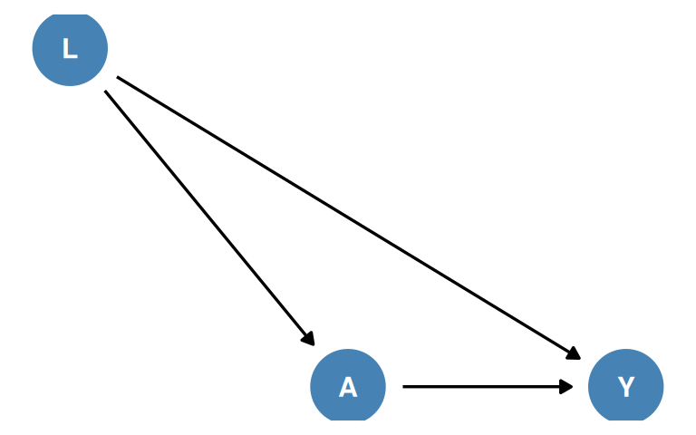
In Figure 7.1 there are two sources of association between \(A\) and \(Y\):

• the causal path \(A \rightarrow Y\);
• the path \(A \leftarrow L \rightarrow Y\) through the common cause \(L\).

The second path begins with an arrow into \(A\) (\(A \leftarrow L\)). (Paths and causal paths are defined in Chapter 6.)

Definition 1 (Backdoor Path) Take a causal DAG with treatment \(A\) and outcome \(Y\). A backdoor path is a noncausal path between \(A\) and \(Y\) that would survive the deletion of every arrow out of \(A\). Equivalently, it begins with an arrow into \(A\) (Hernán and Robins 2020, 91).

Example 2 (The Backdoor Path in Figure 7.1) Deleting the arrow \(A \rightarrow Y\) from Figure 7.1 leaves \(A \leftarrow L \rightarrow Y\) in place, and that path starts with an arrow into \(A\), so it is a backdoor path. The path \(A \rightarrow Y\) is causal, so it is not a backdoor path.

If \(L\) did not exist, all the association between \(A\) and \(Y\) would be causal, and the associational risk ratio \(\Pr[Y = 1 \mid A = 1] / \Pr[Y = 1 \mid A = 0]\) would equal the causal risk ratio \(\Pr[Y^{a=1} = 1] / \Pr[Y^{a=0} = 1]\). The common cause \(L\) adds a second source of association.

Definition 2 (Confounding) Let \(A\) be a treatment and \(Y\) an outcome in a causal DAG. A common cause of \(A\) and \(Y\) is a variable with a directed path to \(A\) that does not pass through \(Y\) and a directed path to \(Y\) that does not pass through \(A\). Confounding is present for the effect of \(A\) on \(Y\) when \(A\) and \(Y\) share a common cause, measured or unmeasured; each common cause opens a backdoor path (Definition 1) between them. The word also names the bias this structure produces: the part of the association between \(A\) and \(Y\) that flows through the open backdoor paths created by their common causes, a form of systematic bias. There is no confounding when \(A\) and \(Y\) share no common cause.

Example 3 (Confounding in Figure 7.1) In Figure 7.1, \(L\) causes both \(A\) and \(Y\). For illustration, let \(L\) be binary, let \(\Pr[A = 1 \mid L = 1] > \Pr[A = 1 \mid L = 0]\) and \(\Pr[Y = 1 \mid L = 1] > \Pr[Y = 1 \mid L = 0]\), and let \(A\) have no effect on \(Y\), so that within each level of \(L\) the treated and the untreated have the same risk, and let both treatment levels occur within each level of \(L\). Then the treated include a larger share of individuals with \(L = 1\) than the untreated do, so their risk is higher, and the associational risk ratio exceeds the causal risk ratio of 1. The gap between them is confounding.

Examples of Confounding

Left: Figure 7.2, in which L causes A, and L and Y share the unmeasured cause U. Right: Figure 7.3, in which L causes Y, and L and A share the unmeasured cause U. Unmeasured nodes are gray.

Example 4 (Confounding Across Fields)  

• Occupational factors (Figure 7.1): physical fitness \(L\) causes both working as a firefighter \(A\) and lower mortality \(Y\) (healthy worker bias).
• Clinical decisions (Figure 7.1 or 7.2): heart disease \(L\) is an indication for aspirin \(A\) and a risk factor for stroke \(Y\), either directly or through unmeasured atherosclerosis \(U\) (confounding by indication or channeling).
• Lifestyle (Figure 7.3): personality and social factors \(U\) lead to both lack of exercise \(A\) and smoking \(L\), which affects death \(Y\).
• Genetic factors (Figure 7.3): a DNA sequence \(L\) that affects trait \(Y\) is more frequent among carriers of sequence \(A\) (linkage disequilibrium or population stratification).
• Social factors (Figure 7.1): disability at age 55 \(L\) affects income at age 65 \(A\) and disability at age 75 \(Y\).
• Environmental exposures (Figure 7.3): weather \(U\) affects levels of particulate matter \(A\) and of other pollutants \(L\) that cause coronary heart disease \(Y\).

In every item a variable (\(L\) or \(U\)) causes both treatment and outcome, so each is an instance of confounding in the sense of Definition 2.

Terminology in the examples:

• “Channeling” is often reserved for bias created by patient-specific risk factors \(L\) that encourage doctors to prescribe a particular drug \(A\) within a class of drugs.
• When subclinical disease \(U\) causes both lack of exercise \(A\) and clinical disease \(Y\), and \(L\) is unknown, this form of confounding is often called reverse causation.
• “Population stratification” is often reserved for bias from studying a mixture of individuals of different ethnic groups, so \(U\) can stand for ethnicity.

Notation: Double-Headed Edges

Some authors draw an unmeasured common cause \(U\) and its two arrows as a single double-headed (bidirected) edge between the two measured variables that \(U\) causes. This chapter keeps \(U\) on the graph, in gray.

Remark 1 (Associations from Common Causes Are Real). Early statistical accounts of confounding dismissed the associations it produces: Yule (1903), writing about discrete variables, called them “fictitious”, “illusory”, and “apparent”, and Pearson et al. (1899), writing about continuous ones, called them “spurious” (Hernán and Robins 2020, 92). Yet such associations are genuine features of the population. What they cannot be is an estimate of the effect of treatment.

Standing Assumptions in This Chapter

Unless stated otherwise, this chapter assumes that

• positivity and consistency hold;
• there are no selection nodes, so the study sample represents the target population;
• every node in a causal diagram is measured without error;
• there is no random variability (the population is infinitely large).

Chapters 8, 9, and 10 relax the last three assumptions in turn (Hernán and Robins 2020, 92–93).

The book reserves the term confounding for the common-cause structure of Definition 2 and uses other names for biases with other structures.

2 7.2 Confounding and Exchangeability (pp. 93-95)

Exchangeability was defined in Chapter 2: marginal exchangeability \(Y^a \perp\!\!\!\perp A\) (Chapter 2) and conditional exchangeability \(Y^a \perp\!\!\!\perp A \mid L\) (Chapter 2). The next three results show what each one identifies.

Proposition 1 (Identification Under Marginal Exchangeability) Let \(A\) be a binary treatment and \(Y\) an outcome. Assume marginal exchangeability \(Y^a \perp\!\!\!\perp A\), positivity \(\Pr[A = a] > 0\), and consistency (\(Y = Y^a\) whenever \(A = a\)), for \(a = 0, 1\). Then \(\operatorname{E}\mathopen{}\left[Y^a\right]\mathclose{} = \operatorname{E}\mathopen{}\left[Y \mid A = a\right]\mathclose{}\) for \(a = 0, 1\), so the average causal effect equals the associational difference:

\[ \operatorname{E}\mathopen{}\left[Y^{a=1}\right]\mathclose{} - \operatorname{E}\mathopen{}\left[Y^{a=0}\right]\mathclose{} = \operatorname{E}\mathopen{}\left[Y \mid A = 1\right]\mathclose{} - \operatorname{E}\mathopen{}\left[Y \mid A = 0\right]\mathclose{} \tag{1}\]

Proof. For each \(a\),

\[\begin{align} \operatorname{E}\mathopen{}\left[Y^a\right]\mathclose{} &= \operatorname{E}\mathopen{}\left[Y^a \mid A = a\right]\mathclose{} && \text{(exchangeability; positivity)} \\ &= \operatorname{E}\mathopen{}\left[Y \mid A = a\right]\mathclose{} && \text{(consistency)} \end{align}\]

Positivity makes the conditional mean in the first line well defined.

Example 5 (A Marginally Randomized Experiment) In a trial in which a coin decides who is treated, nothing causes both \(A\) and \(Y\), so \(Y^a \perp\!\!\!\perp A\) holds by design. If, hypothetically, 30% of the treated and 40% of the untreated die, Proposition 1 gives a causal risk difference of \(0.30 - 0.40 = -0.10\).

Proposition 2 (Stratum-Specific Identification Under Conditional Exchangeability) Let \(A\) be a treatment, \(Y\) an outcome, and \(L\) a discrete set of covariates. Fix a treatment value \(a\) and assume, for this \(a\), conditional exchangeability \(Y^a \perp\!\!\!\perp A \mid L\), positivity \(\Pr[A = a \mid L = l] > 0\) for every \(l\) with \(\Pr[L = l] > 0\), and consistency (\(Y = Y^a\) whenever \(A = a\)). Then, for every such \(l\),

\[ \operatorname{E}\mathopen{}\left[Y^a \mid L = l\right]\mathclose{} = \operatorname{E}\mathopen{}\left[Y \mid L = l, A = a\right]\mathclose{} \tag{2}\]

If the assumptions hold for both \(a = 0\) and \(a = 1\), the conditional effects \(\operatorname{E}\mathopen{}\left[Y^{a=1} \mid L = l\right]\mathclose{} - \operatorname{E}\mathopen{}\left[Y^{a=0} \mid L = l\right]\mathclose{}\) are therefore identified by stratification.

Proof. \[\begin{align} \operatorname{E}\mathopen{}\left[Y^a \mid L = l\right]\mathclose{} &= \operatorname{E}\mathopen{}\left[Y^a \mid L = l, A = a\right]\mathclose{} && \text{(conditional exchangeability; positivity)} \\ &= \operatorname{E}\mathopen{}\left[Y \mid L = l, A = a\right]\mathclose{} && \text{(consistency)} \end{align}\]

Theorem 1 (Standardization Under Conditional Exchangeability) Let \(L\) be a discrete set of covariates and fix a treatment value \(a\). Assume conditional exchangeability \(Y^a \perp\!\!\!\perp A \mid L\), positivity \(\Pr[A = a \mid L = l] > 0\) for every \(l\) with \(\Pr[L = l] > 0\), and consistency (\(Y = Y^a\) whenever \(A = a\)). Then, with the sum over the \(l\) with \(\Pr[L = l] > 0\),

\[\operatorname{E}\mathopen{}\left[Y^a\right]\mathclose{} = \sum_l \operatorname{E}\mathopen{}\left[Y \mid L = l, A = a\right]\mathclose{} \Pr[L = l]\]

Proof. \[\begin{align} \operatorname{E}\mathopen{}\left[Y^a\right]\mathclose{} &= \sum_l \operatorname{E}\mathopen{}\left[Y^a \mid L = l\right]\mathclose{} \Pr[L = l] && \text{(law of total expectation)} \\ &= \sum_l \operatorname{E}\mathopen{}\left[Y \mid L = l, A = a\right]\mathclose{} \Pr[L = l] && \text{(stratum-specific identification)} \end{align}\]

The second line applies Equation 2 of Proposition 2 in each stratum.

Positivity makes every conditional mean in the sums well defined.

Supplement: A Numerical Example

Example 6 (Standardization Removes a Confounded Difference) This hypothetical example is not from the book. Twenty individuals each either receive a drug (\(A = 1\)) or do not (\(A = 0\)); \(L = 1\) indicates a high-risk group; \(Y = 1\) indicates death.

\(L\)	\(A\)	\(n\)	Deaths	\(\Pr[Y = 1 \mid A, L]\)
1	1	8	4	0.50
1	0	2	1	0.50
0	1	2	0	0.00
0	0	8	0	0.00

Crude risks: \(\Pr[Y = 1 \mid A = 1] = (4 + 0) / (8 + 2) = 0.40\) and \(\Pr[Y = 1 \mid A = 0] = (1 + 0) / (2 + 8) = 0.10\).

Assume \(L\) is the only common cause of \(A\) and \(Y\), so that \(Y^a \perp\!\!\!\perp A \mid L\). With \(\Pr[L = 1] = 10/20 = 0.50\), standardization (Theorem 1) gives

\[\begin{align} \Pr[Y^{a=1} = 1] &= 0.50 \times 0.50 + 0.00 \times 0.50 = 0.25 \\ \Pr[Y^{a=0} = 1] &= 0.50 \times 0.50 + 0.00 \times 0.50 = 0.25 \end{align}\]

so the standardized risk difference is \(0\), while the crude risk difference is \(0.40 - 0.10 = 0.30\).

The high-risk group (\(L = 1\)) is treated more often (\(8/10\) versus \(2/10\)) and dies more often (\(0.50\) versus \(0.00\)). Within each level of \(L\) the treated and untreated have the same risk, so the whole crude risk difference of \(0.30\) is confounding.

The Backdoor Criterion

If we know the true causal DAG, how can we tell whether some set \(L\) yields conditional exchangeability? The book gives two approaches: the backdoor criterion (Pearl 1995) and the transformation of the DAG into a single-world intervention graph (SWIG, defined in Section 7.5). The criterion uses blocking: conditioning on a non-collider on a path blocks it, and so does leaving a collider (and its descendants) unconditioned (see d-separation in Chapter 6).

Definition 3 (Backdoor Criterion) A set of covariates \(L\) satisfies the backdoor criterion if

1. all backdoor paths between \(A\) and \(Y\) are blocked by conditioning on \(L\), and
2. \(L\) contains no variables that are descendants of treatment \(A\).

Example 7 (Checking the Backdoor Criterion in Figure 7.1) In Figure 7.1 the only backdoor path is \(A \leftarrow L \rightarrow Y\).

• The set \(\{L\}\) satisfies the criterion: \(L\) is a non-collider on that path, so conditioning on it blocks the path, and \(L\) is not a descendant of \(A\).
• The empty set does not: with nothing conditioned on, the backdoor path stays open.

Theorem 2 (Backdoor Criterion and Conditional Exchangeability) Let \(\mathcal{G}\) be a causal DAG that contains treatment \(A\), outcome \(Y\), a set of covariates \(L\), and possibly other (measured or unmeasured) variables, interpreted as an FFRCISTG model (Chapter 6).

1. If \(L\) satisfies the backdoor criterion (Definition 3), then \(Y^a \perp\!\!\!\perp A \mid L\) for every \(a\).
2. If, in addition, the joint distribution is faithful to \(\mathcal{G}\), then \(Y^a \perp\!\!\!\perp A \mid L\) for every \(a\) only if \(L\) satisfies the backdoor criterion.

Together, under faithfulness, the backdoor criterion for \(L\) and conditional exchangeability given \(L\) are equivalent (Hernán and Robins 2020, 93–94).

The proof is deferred: Section 7.5 sketches a graphical argument for Theorem 2 once SWIGs are defined. Checking every subset of measured non-descendants of \(A\) against the criterion therefore tells us whether any of them achieves conditional exchangeability.

Technical Point 7.1: Does Conditional Exchangeability Imply the Backdoor Criterion?

Part 1 of Theorem 2 needs no faithfulness. Part 2, the converse, depends on the counterfactual model: it holds under an FFRCISTG model (Technical Point 6.3) but can fail under an NPSEM-IE model, as the next example shows. The NPSEM-IE assumes cross-world independencies between counterfactuals, which no randomized experiment could ever verify; for that reason Robins did not assume them in the FFRCISTG model. The book assumes an FFRCISTG model and faithfulness unless stated otherwise (Hernán and Robins 2020, 94).

Example 8 (Conditional Exchangeability Without the Backdoor Criterion) Consider a three-node causal DAG in which \(A\) causes both \(L\) and \(Y\) (\(A \rightarrow L\), \(A \rightarrow Y\)) and there are no other arrows. The set \(\{L\}\) fails the backdoor criterion, because \(L\) is a descendant of \(A\).

• Under an NPSEM-IE, \(Y^a\) depends only on \(a\) and an error term that is independent of the errors generating \(A\) and \(L\), so \(Y^a \perp\!\!\!\perp(A, L)\) and hence \(Y^a \perp\!\!\!\perp A \mid L\).
• Under an FFRCISTG model, conditioning on \(L = l\) among those with \(A = a'\) means conditioning on \(L^{a'} = l\). For \(a' \neq a\), independence of \(Y^a\) and \(L^{a'}\) is a cross-world statement that the model does not impose, so \(Y^a \perp\!\!\!\perp A \mid L\) cannot be assumed.

Two Settings in Which the Backdoor Criterion Holds

Remark 2 (No Confounding, or Confounding That \(L\) Removes).

1. No common causes of treatment and outcome (e.g., Figure 6.2): there are no backdoor paths, the empty set satisfies the criterion, and there is no confounding. This is a marginally randomized experiment; under faithfulness, \(Y^a \perp\!\!\!\perp A\) holds exactly when \(A\) and \(Y\) have no common cause.
2. Common causes, but a set \(L\) of measured non-descendants of \(A\) blocks all backdoor paths (e.g., Figure 7.1): there is confounding, but adjusting for \(L\) removes the bias it causes. This is a conditionally randomized experiment, with an arrow \(L \rightarrow A\) by design.

Definition 4 (Sufficient Set for Confounding Adjustment) Call a set \(L\) of measured variables, none of them a descendant of \(A\), a sufficient set for confounding adjustment if every backdoor path from \(A\) to \(Y\) is blocked once we condition on \(L\). By part 1 of Theorem 2, the treated and the untreated are then exchangeable within levels of \(L\): \(Y^a \perp\!\!\!\perp A \mid L\).

Example 9 (The Heart Transplant Study) The heart transplant study of Chapter 2 was conditionally randomized given a prognostic factor \(L\) (called critical condition in Chapter 2 and severe heart disease in the book’s Chapter 7), which affects both transplant \(A\) and death \(Y\). Critical condition was more common among the treated, so had they gone without a transplant they would still have died more often than the untreated did: the two groups are not marginally exchangeable. Because treatment was randomized within levels of \(L\), they are exchangeable within those levels, and \(\{L\}\) is a sufficient set. This second setting of Remark 2 is also what investigators hope for in observational studies that measure many variables \(L\).

Definition 5 (No Unmeasured Confounding) There is no unmeasured confounding (given \(L\)) when the measured variables include a sufficient set \(L\) for confounding adjustment (Definition 4), so that no backdoor path needs an unmeasured variable to be blocked. There may still be confounding (a common cause of \(A\) and \(Y\) may exist); the point is that \(L\) is enough to block every backdoor path.

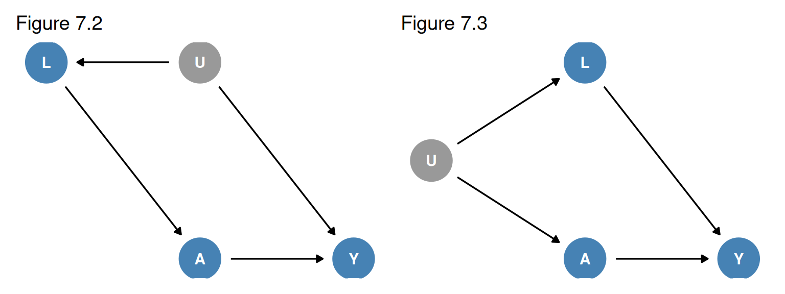
Example 10 (No Unmeasured Confounding in Figure 7.2) In Figure 7.2 the common cause \(U\) of \(A\) and \(Y\) is unmeasured, but the measured \(L\) blocks the only backdoor path, \(A \leftarrow L \leftarrow U \rightarrow Y\), and is not a descendant of \(A\). So \(\{L\}\) is a sufficient set and there is no unmeasured confounding given \(L\), even though there is confounding and \(U\) was never recorded.

The Backdoor Criterion Is Silent on Size and Sign

The criterion says whether an open backdoor path exists, not how much bias it causes or which way the bias goes. An open backdoor path may carry only a weak association, and two strong open paths may push the estimate in opposite directions and partly cancel. Unmeasured confounding comes in degrees, so investigators should think about its likely direction and magnitude (Fine Point 7.1).

The book refers to Greenland and Robins (1986, 2009) for a detailed discussion of the relations between confounding and exchangeability.

3 7.3 Confounding and the Backdoor Criterion (pp. 95-98)

Example 11 (The Backdoor Criterion in Figures 7.1-7.3)  

• Figure 7.1: the backdoor path \(A \leftarrow L \rightarrow Y\) is blocked by conditioning on \(L\).
• Figure 7.2: the backdoor path \(A \leftarrow L \leftarrow U \rightarrow Y\) could be blocked by \(U\), which is unmeasured, but it is also blocked by \(L\).
• Figure 7.3: the backdoor path \(A \leftarrow U \rightarrow L \rightarrow Y\) is also blocked by \(L\).

In all three there is confounding, but \(\{L\}\) is a sufficient set, so there is no unmeasured confounding given \(L\) (Definition 5).

M-bias: Figure 7.4

Left: Figure 7.4, in which L is a collider on the path A <- U2 -> L <- U1 -> Y. Right: Figure 7.5, which adds the arrow L -> A.

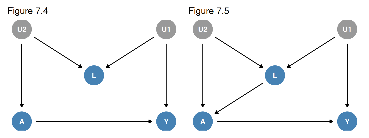
Example 12 (No Confounding in Figure 7.4) In Figure 7.4 \(A\) and \(Y\) share no common cause, so there is no confounding. The only backdoor path, \(A \leftarrow U_2 \rightarrow L \leftarrow U_1 \rightarrow Y\), is blocked by the unconditioned collider \(L\), so the empty set satisfies the backdoor criterion and Theorem 2 gives \(Y^a \perp\!\!\!\perp A\). With positivity and consistency, Proposition 1 then gives \(\Pr[Y^a = 1] = \Pr[Y = 1 \mid A = a]\).

Example 13 (Physical Activity and Cervical Cancer) Let \(A\) be physical activity, \(Y\) cervical cancer, \(U_1\) a pre-cancer lesion, \(L\) a Pap smear (a diagnostic test for pre-cancer), and \(U_2\) a health-conscious personality that leads to more physical activity and more doctor visits. Under Figure 7.4 the effect of \(A\) on \(Y\) is unconfounded, and there is no need to adjust for \(L\) to compute \(\Pr[Y^{a=1} = 1]\) or \(\Pr[Y^{a=0} = 1]\) (Hernán and Robins 2020, 95).

Adjusting for a Collider Creates Bias

In Figure 7.4, conditioning on the collider \(L\) opens the path \(A \leftarrow U_2 \rightarrow L \leftarrow U_1 \rightarrow Y\), so adjusting for \(L\) (by stratification or by standardization over \(L\)) creates bias where there was none.

Definition 6 (M-bias) M-bias is the bias that arises from conditioning on a variable \(L\) that is a common effect of two variables \(U_1\) and \(U_2\), where \(U_2\) is a cause of treatment \(A\), \(U_1\) is a cause of the outcome \(Y\), \(U_1\) and \(U_2\) are marginally independent, and \(A\) and \(Y\) share no common cause (as in Figure 7.4). The book classifies it as a form of selection bias, the subject of Chapter 8 (Hernán and Robins 2020, 97).

Example 14 (M-bias in the Pap Smear Example) In Example 13, comparing physical activity and cervical cancer only among women with the same Pap smear result conditions on \(L\), a common effect of the pre-cancer lesion \(U_1\) and of health-conscious personality \(U_2\). Within a stratum of \(L\), physical activity and cervical cancer generally become associated through \(U_2\) and \(U_1\), so the stratum-specific association mixes the causal effect with bias, even though the unadjusted comparison is unconfounded and equals the causal contrast.

Remark 3 (Unconditional Without Conditional Exchangeability). In Figure 7.4, \(Y^a \perp\!\!\!\perp A\) holds but, under faithfulness, \(Y^a \perp\!\!\!\perp A \mid L\) does not. The average causal effect is identified by Proposition 1, but the effects within levels of \(L\) are generally not identified by adjusting for \(L\), and standardizing over \(L\) generally gives a biased estimate of \(\Pr[Y^a = 1]\).

Why “M-bias”: the structure was described by Greenland, Pearl, and Robins (1999) and named M-bias by Greenland (2003), because \(U_2\), \(L\), \(U_1\) resemble an M lying on its side (Hernán and Robins 2020, 97). That unconditional effects can be identified while conditional effects are not was shown non-graphically by Greenland and Robins (1986).

If \(U_1\) caused \(U_2\), \(U_2\) caused \(U_1\), or an unmeasured \(U_3\) caused both, \(A\) and \(Y\) would have a common cause, and there would be neither unconditional nor conditional exchangeability given \(L\).

Intractable Bias: Figure 7.5

Example 15 (Intractable Bias in Figure 7.5) Figure 7.5 adds the arrow \(L \rightarrow A\), which creates the open backdoor path \(A \leftarrow L \leftarrow U_1 \rightarrow Y\): there is confounding.

• Conditioning on \(L\) blocks \(A \leftarrow L \leftarrow U_1 \rightarrow Y\),
• but opens \(A \leftarrow U_2 \rightarrow L \leftarrow U_1 \rightarrow Y\), on which \(L\) is a collider.

So neither the empty set nor \(\{L\}\) satisfies the backdoor criterion, and, by Theorem 2 under faithfulness, exchangeability fails both marginally and within levels of \(L\).

Being a Collider Is Path-Specific

In Figure 7.5, \(L\) is a collider on \(A \leftarrow U_2 \rightarrow L \leftarrow U_1 \rightarrow Y\) but a non-collider on \(A \leftarrow L \leftarrow U_1 \rightarrow Y\). A variable is a collider only relative to a given path.

Remark 4 (Intermediate Variables That Restore Exchangeability). Measuring more variables in Figure 7.5 as drawn does not help. But if the arrows \(U_1 \rightarrow Y\) and \(U_2 \rightarrow A\) in fact pass through measurable intermediate variables, measuring those can remove the bias.

Figure 7.6 (not drawn here) is Figure 7.5 with the arrow \(U_1 \rightarrow Y\) replaced by \(U_1 \rightarrow L_1 \rightarrow Y\) and the arrow \(U_2 \rightarrow A\) replaced by \(U_2 \rightarrow L_2 \rightarrow A\). In Figure 7.6,

• measuring \(L_1\) gives conditional exchangeability given \(L_1\), because \(L_1\) blocks every backdoor path at its end near \(Y\);
• measuring \(L_2\) (with \(L\)) gives conditional exchangeability given \(\{L_2, L\}\), because \(L\) blocks \(A \leftarrow L \leftarrow U_1 \rightarrow L_1 \rightarrow Y\) and \(L_2\) blocks the path that conditioning on \(L\) opens.

Fine Point 7.1: The Strength and Direction of Confounding Bias

Knowing that confounding may be present is only half the story: investigators also want to know whether the unadjusted estimate is too large or too small, and by how much. The boxes that follow define signed causal diagrams, which give a rule of thumb for the direction, apply the rule to an example, and discuss the magnitude (Hernán and Robins 2020, 96).

Definition 7 (Signed Causal Diagram; Positive and Negative Confounding) Let \(L\), \(A\), and \(Y\) be binary and related as in Figure 7.1. A signed causal diagram labels the arrow \(L \rightarrow A\) with \(+\) when \(L = 1\) makes \(A = 1\) more likely on average than \(L = 0\) does, and with \(-\) when it makes \(A = 1\) less likely, and signs the arrow \(L \rightarrow Y\) in the same way. The confounding is called positive if the two signs agree and negative if they differ.

Example 16 (Smoking and Heart Transplant) Suppose a study of heart transplant \(A\) on death \(Y\) finds a risk ratio of 0.6, and a critic suspects confounding by smoking \(L\). Smokers are less likely to receive a transplant (\(L \rightarrow A\) is \(-\)) and more likely to die (\(L \rightarrow Y\) is \(+\)), so the confounding is negative in the sense of Definition 7. Because the transplant group has fewer smokers, it would have lower mortality even if transplant did nothing, so adjusting for smoking moves the estimate upward (the book’s illustration: from 0.6 to 0.7). Failing to adjust exaggerates the apparent benefit.

Remark 5 (The Sign Rule). Let \(L\), \(A\), and \(Y\) be binary and related as in Figure 7.1, with \(L\) the only common cause of \(A\) and \(Y\), and call the bias the unadjusted risk ratio minus the risk ratio standardized over \(L\). The book’s rule of thumb is that positive confounding biases the unadjusted estimate upward and negative confounding biases it downward (Hernán and Robins 2020, 96). In Example 16 the confounding is negative, and indeed the unadjusted 0.6 lies below the adjusted 0.7.

The Sign Rule Can Fail

The rule of Remark 5 may fail in more complex diagrams or with non-dichotomous variables (VanderWeele, Hernán, and Robins 2008).

Remark 6 (The Magnitude of Confounding Bias). A common cause \(L\) produces a large confounding bias only if it is strongly associated with treatment and strongly associated with the outcome (conditional on treatment); for a discrete \(L\), the bias also depends on how common it is. When the common causes are unknown, sensitivity analyses repeat the analysis under a range of assumed bias sizes, which organizes educated guesses about how large the bias could plausibly be (Hernán and Robins 2020, 96).

Confounders and Non-confounders

Suppose data on \(L\), \(A\), and \(Y\) suffice to identify the causal effect, as in Figures 7.1-7.4.

Definition 8 (Confounder (Given Data on L, A, Y)) \(L\) is a confounder if data on \(A\) and \(Y\) alone do not suffice for identification, that is, if there is conditional exchangeability given \(L\) but not unconditional exchangeability (structural confounding). \(L\) is a non-confounder if data on \(A\) and \(Y\) alone suffice, that is, if there is unconditional exchangeability (Hernán and Robins 2020, 96).

Example 17 (Confounders and Non-confounders in Figures 7.1-7.4)  

• In Figures 7.1-7.3, \(L\) is a confounder: \(\Pr[Y^a = 1]\) is identified by the standardized risk \(\sum_l \Pr[Y = 1 \mid A = a, L = l] \Pr[L = l]\) (Theorem 1). In Figures 7.2 and 7.3, \(L\) is not a common cause of \(A\) and \(Y\), yet it is a confounder because it is needed to block the backdoor path through \(U\).
• In Figure 7.4, \(L\) is a non-confounder, and \(\Pr[Y^a = 1] = \Pr[Y = 1 \mid A = a]\). Standardizing by \(L\) would be biased.

An informal definition for Figures 7.1 to 7.4 is “a confounder is any variable that can be used to adjust for confounding.” This definition is not circular, because confounding was defined first, just as “a musician is a person who plays music” is not circular once music has been defined (Hernán and Robins 2020, 96).

Two Definitions of Confounding

The causal diagrams of this section show two structural sources of lack of exchangeability through open backdoor paths:

• common causes of treatment and outcome, which the book calls confounding (Definition 2);
• conditioning on a common effect, which the book calls selection bias (as in Definition 6).

Definition 9 (Confounding as Any Open-Backdoor-Path Bias) An alternative structural definition calls confounding any bias that an open backdoor path between \(A\) and \(Y\) produces, whether the path is open because of a common cause or because of conditioning on a collider. Equivalently, confounding is any systematic bias that randomized assignment of \(A\) would eliminate.

Example 18 (Figure 7.4 Under the Two Definitions) In Figure 7.4, the bias from adjusting for \(L\) is not confounding under Definition 2 (the book calls it selection bias, as in Definition 6) but is confounding under Definition 9. Randomizing \(A\) would remove it: with \(A\) assigned by a coin, the arrow \(U_2 \rightarrow A\) disappears, so stratifying on \(L\) leaves every path from \(A\) to \(Y\) other than \(A \rightarrow Y\) closed. The common-cause bias of Figures 7.1-7.3 is confounding under both definitions.

Remark 7 (The Choice of Definition Has No Practical Consequences). Under Definition 2, whether confounding exists is a fact about the population, whatever the analysis. Under Definition 9 it depends on the analysis: in Figure 7.4 there is no confounding if we do not adjust for \(L\), but there is if we do. Either way, what can be identified depends only on whether conditional or unconditional exchangeability holds, so the choice is a matter of taste (Hernán and Robins 2020, 98).

Fine Point 7.2: Identification of Conditional and Unconditional Effects

Which effects can be identified depends on which variables are measured besides \(A\) and \(Y\). The next example works this out for Figure 7.6 (Remark 4) (Hernán and Robins 2020, 98).

Example 19 (What Can Be Identified in Figure 7.6)  

• Measuring only \(L_2\): no exchangeability given \(L_2\); no causal effects are identified.
• Measuring \(L_2\) and \(L\): conditional exchangeability given \(\{L_2, L\}\) (but not given either alone). Identified are:
  • effects within joint strata of \(L\) and \(L_2\), via \(\operatorname{E}\mathopen{}\left[Y \mid A = a, L = l, L_2 = l_2\right]\mathclose{}\);
  • the unconditional effect, via \(\sum_{l, l_2} \operatorname{E}\mathopen{}\left[Y \mid A = a, L = l, L_2 = l_2\right]\mathclose{} \Pr[L = l, L_2 = l_2]\);
  • effects within strata of \(L\), via \(\sum_{l_2} \operatorname{E}\mathopen{}\left[Y \mid A = a, L = l, L_2 = l_2\right]\mathclose{} \Pr[L_2 = l_2 \mid L = l]\);
  • effects within strata of \(L_2\), via \(\sum_{l} \operatorname{E}\mathopen{}\left[Y \mid A = a, L = l, L_2 = l_2\right]\mathclose{} \Pr[L = l \mid L_2 = l_2]\).
• Measuring only \(L_1\): effects within strata of \(L_1\) and the unconditional effect.
• Measuring \(L_1\) and \(L\): additionally, effects within joint strata of \(L_1\) and \(L\), and within strata of \(L\).
• Measuring \(L\), \(L_1\), and \(L_2\): additionally, effects within joint strata of all three.

Each formula identifies a counterfactual mean \(\operatorname{E}\mathopen{}\left[Y^a \mid \cdot\right]\mathclose{}\) under positivity, consistency, and conditional exchangeability given the measured set (which holds for \(\{L_1\}\), \(\{L_1, L\}\), \(\{L_2, L\}\), and \(\{L, L_1, L_2\}\) by the backdoor criterion in Figure 7.6).

4 7.4 Confounding and Confounders (pp. 98-101)

The structural approach needs prior knowledge of the causal DAG, including all shared causes (measured or not) of \(A\) and \(Y\); the backdoor criterion then says what to adjust for. The traditional approach instead labels as confounders the variables meeting mostly associational conditions, mandates adjusting for them, and declares confounding when adjusted and unadjusted estimates differ.

Definition 10 (Traditional Definition of Confounder) A variable is a confounder under the traditional approach if it

1. is associated with the treatment,
2. is associated with the outcome conditional on the treatment (often replaced by “in the untreated”), and
3. does not lie on a causal pathway between treatment and outcome.

Example 20 (Where the Traditional Approach Agrees and Disagrees)  

• Figures 7.1-7.3: \(L\) meets all three conditions, matching the backdoor criterion.
• Figure 7.4: \(L\) meets all three conditions (it shares \(U_2\) with \(A\) and \(U_1\) with \(Y\), and is not on the causal pathway), so the traditional approach says to adjust for it, although there is no confounding and adjusting causes selection bias.
• Figure 7.7 (not drawn here) is a second example in which the traditional approach leads to harmful adjustment for \(L\).

Remark 8 (Patching Condition 2 Does Not Work). Replacing condition 2 of Definition 10 by the structural condition “it is a cause of the outcome” fixes Figure 7.4, but then \(L\) in Figure 7.2 would no longer count as a confounder, although it must be adjusted for. Technical Point 7.2 gives a replacement that handles Figures 7.4 and 7.7.

Associations Cannot Define Confounding

A definition of confounder built almost entirely on statistical associations can advise adjusting for a “confounder” when no structural confounding exists. Nor does a change in estimate after adjustment prove confounding: adjusted and unadjusted estimates can differ because adjustment for a non-confounder created selection bias (Chapter 8), or because the effect measure is noncollapsible (Fine Point 4.3). Definitions of confounding based on change in estimates were abandoned long ago for these reasons (Hernán and Robins 2020, 100).

Strictly speaking, investigators do not need the whole causal structure; it is enough to know some set of variables that delivers conditional exchangeability.

Confounding Is Absolute; Confounder Is Relative

Remark 9 (Whether a Variable Is a Confounder Depends on the Adjustment Set). The structural approach first identifies the sources of confounding (the common causes of treatment and outcome) and then a sufficient adjustment set. Whether a variable belongs to a sufficient set depends on the other variables in it. In Figures 7.2 and 7.3, \(L\) is needed only because \(U\) is unmeasured; given \(U\), \(L\) would not be a confounder. So, for a given causal DAG, whether there is confounding is a fixed fact, while whether a variable is a confounder depends on what else is adjusted for (Hernán and Robins 2020, 100).

Remark 10 (Two Advantages of the Structural Approach).

1. It prevents inconsistencies between beliefs and actions: if you believe Figure 7.4, you will not adjust for \(L\), whatever a non-structural definition says.
2. It makes the researchers’ assumptions explicit, so others can criticize them.

VanderWeele and Shpitser (2013) also proposed a formal definition of confounder. No approach guarantees that the researchers’ DAG is correct, so a chosen adjustment set may still fail to remove confounding or may introduce selection bias.

Figure 7.8. L is a surrogate (proxy) for the unmeasured common cause U of A and Y.

Fine Point 7.3: Surrogate Confounders

A measured variable can help with confounding without lying on any backdoor path. The boxes that follow name such variables and give an example (Hernán and Robins 2020, 100).

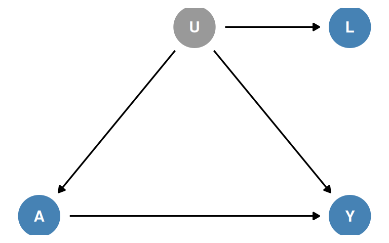
Definition 11 (Surrogate Confounder) A surrogate confounder is a measured non-descendant \(L\) of \(A\) that lies on no backdoor path from \(A\) to \(Y\) but is a proxy for (for example, an effect of) an unmeasured common cause \(U\) of \(A\) and \(Y\), as in Figure 7.8. Adjusting for \(L\) typically reduces the confounding by \(U\), but because \(L\) blocks no backdoor path it generally cannot remove all of it.

Example 21 (Income as a Surrogate for Socioeconomic Status) In Figure 7.8 the unmeasured \(U\) (e.g., socioeconomic status) confounds the effect of physical activity \(A\) on cardiovascular disease \(Y\), and the measured \(L\) (e.g., income) is a proxy for \(U\). \(L\) is not on a backdoor path, but adjusting for it may remove some of the confounding by \(U\); if \(L\) were perfectly correlated with \(U\), conditioning on \(L\) would be the same as conditioning on \(U\). If \(L\) is a binary, nondifferentially misclassified version of \(U\), conditioning on \(L\) partially blocks \(A \leftarrow U \rightarrow Y\) under some weak conditions (Greenland 1980; Ogburn and VanderWeele 2012). So one typically prefers to adjust for \(L\).

Collect Many Surrogates

One strategy against unmeasured confounding is to measure and adjust for as many surrogate confounders as possible (see Chapter 18).

Technical Point 7.2: Fixing the Traditional Definition of Confounder

In the traditional definition (Definition 10), conditions 1 and 2 are statistical and condition 3 is causal, and all three are wrong. The boxes that follow replace them, following Robins (1997, Theorem 4.3) and Greenland, Pearl, and Robins (1999), show what the replacement buys, and apply it to Figure 7.4 (Hernán and Robins 2020, 101).

Definition 12 (Non-confounder Given Data on L) Let \(L\) (measured) and \(U\) (possibly unmeasured) be sets of non-descendants of \(A\) with conditional exchangeability \(Y^a \perp\!\!\!\perp A \mid L, U\). \(U\) is a non-confounder given data on \(L\) if \(U\) can be split into disjoint subsets \(U_1\) and \(U_2\) (\(U = U_1 \cup U_2\), \(U_1 \cap U_2 = \emptyset\)) such that

1. given \(L\), \(U_1\) is independent of treatment: \(U_1 \perp\!\!\!\perp A \mid L\), and
2. given \(A\), \(L\), and \(U_1\), \(U_2\) is independent of the outcome: \(U_2 \perp\!\!\!\perp Y \mid A, L, U_1\).

\(U_1\) and \(U_2\) may be associated with each other.

Example 22 (Figure 7.4 via the Non-confounder Condition) In Figure 7.4 take \(L = \emptyset\) (adjust for nothing) and \(U = \{U_1, U_2\}\). The set \(\{U_1, U_2\}\) blocks the only backdoor path at \(U_2\) and contains no descendant of \(A\), so Theorem 2 gives \(Y^a \perp\!\!\!\perp A \mid U_1, U_2\), the premise of Definition 12. Assume \(U_1\) and \(U_2\) are discrete, and assume consistency and \(\Pr[A = a \mid U_1, U_2] > 0\). The two conditions of Definition 12 hold, with the subsets named as in the figure:

1. \(U_1 \perp\!\!\!\perp A\): the two paths between them, \(U_1 \rightarrow L \leftarrow U_2 \rightarrow A\) and \(U_1 \rightarrow Y \leftarrow A\), each pass through a collider (\(L\) or \(Y\)) that is not conditioned on.
2. \(U_2 \perp\!\!\!\perp Y \mid A, U_1\): the path \(U_2 \rightarrow A \rightarrow Y\) is blocked by conditioning on \(A\), and \(U_2 \rightarrow L \leftarrow U_1 \rightarrow Y\) is blocked by the unconditioned collider \(L\) and by \(U_1\).

Both independence statements are read off the DAG by d-separation, which implies independence under the causal Markov assumption. So \(\{U_1, U_2\}\) is a non-confounder given data on \(L = \emptyset\).

Proposition 3 (Adjusting for L Alone Suffices) Let \(L\) and \(U\) be discrete sets of non-descendants of \(A\) with \(Y^a \perp\!\!\!\perp A \mid L, U\), and suppose \(U\) is a non-confounder given data on \(L\) (Definition 12), with split \(U = U_1 \cup U_2\). Fix a treatment value \(a\) and assume consistency and positivity, \(\Pr[A = a \mid L = l, U = u] > 0\) for every \((l, u)\) with \(\Pr[L = l, U = u] > 0\). Then, for every \(l\) with \(\Pr[L = l] > 0\),

\[ \operatorname{E}\mathopen{}\left[Y^a \mid L = l\right]\mathclose{} = \operatorname{E}\mathopen{}\left[Y \mid A = a, L = l\right]\mathclose{} \tag{3}\]

so \(\operatorname{E}\mathopen{}\left[Y^a\right]\mathclose{} = \sum_l \operatorname{E}\mathopen{}\left[Y \mid A = a, L = l\right]\mathclose{} \Pr[L = l]\): standardization over \(L\) alone identifies the counterfactual mean.

Proof. This derivation is ours, not the book’s. Let \(\mu(u_1)\) denote \(\operatorname{E}\mathopen{}\left[Y \mid A = a, L = l, U_1 = u_1\right]\mathclose{}\). By condition 2, \(\operatorname{E}\mathopen{}\left[Y \mid A = a, L = l, U_1 = u_1, U_2 = u_2\right]\mathclose{} = \mu(u_1)\). First, by the law of total expectation, conditional exchangeability, and consistency,

\[\begin{align} \operatorname{E}\mathopen{}\left[Y^a \mid L = l\right]\mathclose{} &= \sum_{u} \operatorname{E}\mathopen{}\left[Y^a \mid L = l, U = u\right]\mathclose{} \Pr[U = u \mid L = l] \\ &= \sum_{u} \operatorname{E}\mathopen{}\left[Y \mid A = a, L = l, U = u\right]\mathclose{} \Pr[U = u \mid L = l] \\ &= \sum_{u_1} \mu(u_1) \Pr[U_1 = u_1 \mid L = l] \end{align}\]

Second, by the law of total expectation and condition 2,

\[\begin{align} \operatorname{E}\mathopen{}\left[Y \mid A = a, L = l\right]\mathclose{} &= \sum_{u} \operatorname{E}\mathopen{}\left[Y \mid A = a, L = l, U = u\right]\mathclose{} \Pr[U = u \mid A = a, L = l] \\ &= \sum_{u_1} \mu(u_1) \Pr[U_1 = u_1 \mid A = a, L = l] \\ &= \sum_{u_1} \mu(u_1) \Pr[U_1 = u_1 \mid L = l] \end{align}\]

where the last line uses condition 1. The two right-hand sides agree, which proves Equation 3; averaging over \(\Pr[L = l]\) gives the formula for \(\operatorname{E}\mathopen{}\left[Y^a\right]\mathclose{}\).

Applied to Example 22, Proposition 3 gives \(\operatorname{E}\mathopen{}\left[Y^a\right]\mathclose{} = \operatorname{E}\mathopen{}\left[Y \mid A = a\right]\mathclose{}\): there is no confounding in Figure 7.4, as the backdoor criterion showed in Example 12.

5 7.5 Single-World Intervention Graphs (pp. 101-102)

The equivalence between exchangeability and the backdoor criterion seems “rather magical” because counterfactuals do not appear on causal diagrams. Single-world intervention graphs (SWIGs) put the counterfactual variables on the graph, so that exchangeability can be read off directly by d-separation.

Definition 13 (Single-World Intervention Graph (SWIG)) A SWIG depicts the variables and causal relations that would be observed in a hypothetical world in which all individuals received treatment level \(a\), a counterfactual world created by a single intervention. It is obtained from a causal DAG as follows:

• Split the treatment node into a left side \(A\) (the natural value of treatment, the value that would have been observed without intervention), which keeps all arrows into \(A\), and a right side \(a\) (the intervention value), which inherits all arrows out of \(A\). There is no arrow from \(A\) to \(a\), because \(a\) is a constant.
• Replace each descendant of treatment by its counterfactual, e.g., \(Y\) by \(Y^a\). Non-descendants of \(A\) keep their factual labels, because treatment does not affect them.

Example 23 (SWIGs for Figures 7.2 and 7.4)  

• Figure 7.9 is the SWIG of Figure 7.2: \(U \rightarrow L \rightarrow A\), \(U \rightarrow Y^a\), \(a \rightarrow Y^a\). Every path between \(Y^a\) and \(A\) is blocked by conditioning on \(L\), so \(Y^a \perp\!\!\!\perp A \mid L\).
• Figure 7.10 is the SWIG of Figure 7.4: \(U_2 \rightarrow A\), \(U_2 \rightarrow L \leftarrow U_1 \rightarrow Y^a\), \(a \rightarrow Y^a\). Without conditioning, the path through the collider \(L\) is blocked, so \(Y^a \perp\!\!\!\perp A\). Conditioning on \(L\) opens \(Y^a \leftarrow U_1 \rightarrow L \leftarrow U_2 \rightarrow A\), so \(Y^a \perp\!\!\!\perp A \mid L\) fails.

Proof (Sketch of a proof of Theorem 2). On the SWIG, \(Y^a\) and \(A\) are d-separated given \(L\) exactly when \(L\) contains no descendant of \(A\) and blocks every backdoor path between \(A\) and \(Y\) (Hernán and Robins 2020, 102): the natural value \(A\) keeps only the arrows into treatment, so every path between \(A\) and \(Y^a\) starts with an arrow into \(A\), as a backdoor path does, and a descendant of \(A\) appears on the SWIG only as a counterfactual, so the factual variable cannot be in the conditioning set. Under an FFRCISTG model, d-separation on the SWIG implies \(Y^a \perp\!\!\!\perp A \mid L\), which gives part 1. For part 2 with a set \(L\) of non-descendants, if some backdoor path stays open given \(L\), then \(Y^a\) and \(A\) are not d-separated given \(L\) on the SWIG, and faithfulness turns that into dependence. When \(L\) contains a descendant of \(A\), the SWIG does not display the independence; that case of part 2 is taken from the book (Technical Point 7.1), not proved here. This is a sketch, not a full proof.

Notation: Arrows Out of the Intervention Node

In the single-intervention world, \(a\) is a constant and cannot affect other variables. SWIGs still draw arrows from \(a\), to keep track of which variables \(A\) directly affects in the original DAG.

Origins: Richardson and Robins (2013) showed that SWIGs overcome some shortcomings of the twin causal diagrams previously proposed by Balke and Pearl (1994) (Hernán and Robins 2020, 101).

Is the natural value measurable? The book assumes the natural value \(A\) is well defined even though it is generally not observed under intervention \(a\). It notes experiments suggesting that electroencephalogram recordings can detect a choice up to 1/2 second before people become conscious of it, which in principle would allow measuring \(A\) and still intervening.

6 7.6 Confounding Adjustment (pp. 102-107)

Without randomization, causal inference relies on the uncheckable assumption that the measured \(L\) is a sufficient set for confounding adjustment (Definition 4). Under that assumption, methods that adjust for \(L\) fall into two categories, both of which rely on conditional exchangeability given \(L\).

Definition 14 (G-methods and Conventional Stratification-Based Methods)  

• G-methods (“g” for generalized) are standardization, IP weighting, and g-estimation: methods whose target is the causal effect in the whole population or in any subset of it.
• Conventional stratification-based methods are stratification (including restriction) and matching: methods whose target is the \(A\)-\(Y\) association within subsets defined by \(L\).

Example 24 (Both Kinds of Method in the Heart Transplant Study) Earlier chapters handled confounding by disease severity \(L\) in the heart transplant study both ways: with g-methods (standardization and IP weighting in Chapter 2) and with conventional methods (stratification and matching in Chapter 4). Part II extends both kinds with models: the g-methods to the parametric g-formula, marginal structural models, and structural nested models, and the conventional methods to outcome regression.

Remark 11 (“Deleting” an Arrow Versus Conditioning). Standardization and IP weighting reproduce the \(A\)-\(Y\) association that the population would show if no backdoor path ran through \(L\); IP weighting, for example, creates a pseudo-population in which \(A\) is independent of \(L\), “deleting” the arrow \(L \rightarrow A\). Stratification does not delete that arrow but computes the effect in a subset, represented by a selection box. Part III explains why deleting the arrow is advantageous with time-varying treatments, why g-estimation, a g-method that like stratification works within levels of the covariates, remains valid in general when stratification and matching do not, and why conventional stratification-based methods can cause selection bias with time-varying confounders (Chapter 20).

A common variation of stratification and matching replaces \(L\) by the estimated probability of treatment \(\Pr[A = 1 \mid L]\), the propensity score (Rosenbaum and Rubin 1983; Chapter 15).

Fine Point 7.4: Confounders Cannot Be Descendants of Treatment, but Can Be in the Future of Treatment

The backdoor criterion excludes descendants of \(A\), not variables measured after \(A\). The example that follows shows why descendants are excluded, and the remark after it shows that timing alone does not matter (Hernán and Robins 2020, 103).

Example 25 (A Descendant That Blocks Every Backdoor Path (Figure 7.11)) Figure 7.11 (not drawn here) has arrows \(U \rightarrow A\), \(U \rightarrow L\), \(A \rightarrow L\), and \(L \rightarrow Y\), with \(U\) unmeasured. \(L\) is a descendant of \(A\) that blocks the only backdoor path, \(A \leftarrow U \rightarrow L \rightarrow Y\), and the effect of \(A\) on \(Y\) is entirely through \(L\). Conditioning on \(L\) opens no path between \(A\) and \(Y\) through a collider, but it blocks the causal pathway. Because \(Y\) depends on \(A\) and \(U\) only through \(L\), \(Y \perp\!\!\!\perp A \mid L\), so the standardized risk \(\sum_l \Pr[Y = 1 \mid A = a, L = l] \Pr[L = l]\) is the same for \(a = 0\) and \(a = 1\): adjusting for \(L\) shows no effect however large the true effect is. If \(Y^a \perp\!\!\!\perp A \mid L\) held, then with positivity and consistency standardization would recover \(\operatorname{E}\mathopen{}\left[Y^a\right]\mathclose{}\) (Theorem 1), so \(\operatorname{E}\mathopen{}\left[Y^{a=1}\right]\mathclose{}\) and \(\operatorname{E}\mathopen{}\left[Y^{a=0}\right]\mathclose{}\) would be equal. Hence, whenever \(\operatorname{E}\mathopen{}\left[Y^{a=1}\right]\mathclose{} \neq \operatorname{E}\mathopen{}\left[Y^{a=0}\right]\mathclose{}\) (and positivity holds), conditional exchangeability \(Y^a \perp\!\!\!\perp A \mid L\) fails. On the SWIG (Figure 7.12: \(U \rightarrow A\), \(U \rightarrow L^a\), \(a \rightarrow L^a \rightarrow Y^a\)) \(L\) is replaced by the counterfactual \(L^a\), and we can read off \(Y^a \perp\!\!\!\perp A \mid L^a\) but not \(Y^a \perp\!\!\!\perp A \mid L\), since \(L\) is not on the graph. (Under an FFRCISTG model, an independence that cannot be read off the SWIG cannot be assumed to hold.)

Remark 12 (Topology, Not Timing). The problem in Example 25 is that \(L\) is a descendant of \(A\), not that \(L\) occurs after \(A\). Without the arrow \(A \rightarrow L\), \(L\) would be a non-descendant that blocks all backdoor paths, and adjusting for it would remove all bias even if \(L\) were measured after \(A\). Only which variables cause which matters, not when they are measured (Hernán and Robins 2020, 103).

Methods That Do Not Require Conditional Exchangeability

Some methods handle confounding without conditional exchangeability:

• difference-in-differences and negative outcome controls (Technical Point 7.3);
• proximal inference (Technical Point 7.3);
• the front door criterion (Technical Point 7.4);
• instrumental variable estimation (Chapter 16).

Other Methods Need Other Unverifiable Assumptions

These methods replace conditional exchangeability with other assumptions that are just as unverifiable, so the choice of method depends on which unverifiable assumptions are more plausible in a given setting.

Expert Knowledge and the Critic

Use Expert Knowledge of the Causal Structure

Conditional exchangeability may be unrealistic, but expert knowledge about the causal structure helps get close to it:

• measure many non-descendants \(L\) of treatment in the hope of blocking all backdoor paths;
• avoid adjusting for variables affected by treatment or by the outcome;
• when several causal structures are plausible, analyze under each and state the assumptions each requires.

Example 26 (A Logical Versus a Scientific Criticism) A critic who says only “your observational study may be confounded” makes a logical, not a scientific, statement: it is true of every observational study. A scientific criticism names a source, such as “confounding due to cigarette smoking, a common cause through which a backdoor path may remain open”. That gives a testable challenge: adjust for smoking or, if smoking was not measured, conduct a sensitivity analysis (Hernán and Robins 2020, 104–5).

Hernán et al. (2002) give a practical example of using expert knowledge of the causal structure to evaluate confounding. One can never be certain that the causal structures considered include the true one; this uncertainty is unavoidable with observational data.

Valid causal inference from observational data also requires the absence of selection and measurement biases, which, unlike confounding, can arise in randomized experiments too. Chapter 8 turns to selection bias.

Left: Figure 7.13, with negative outcome control C (the pre-treatment outcome). Right: Figure 7.14, in which M fully mediates the effect of A on Y. U is unmeasured.

Technical Point 7.3: Difference-in-Differences and Negative Outcome Controls

A variable that treatment cannot affect but that shares the unmeasured confounders of the outcome can measure the confounding. The boxes that follow define negative outcome controls and additive equi-confounding, give the resulting identification result with an example, and point to a more general approach (Hernán and Robins 2020, 106).

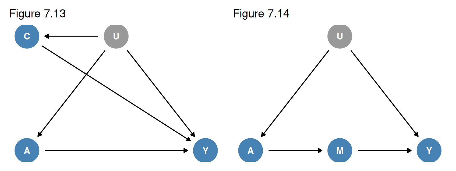
Definition 15 (Negative Outcome Control) A negative outcome control for the effect of \(A\) on \(Y\) is a variable \(C\) that \(A\) cannot cause but that shares the unmeasured causes \(U\) of \(A\) and \(Y\) (Figure 7.13). The outcome measured just before treatment is the usual example. Because \(A\) has no effect on \(C\), \(\operatorname{E}\mathopen{}\left[C \mid A = 1\right]\mathclose{} - \operatorname{E}\mathopen{}\left[C \mid A = 0\right]\mathclose{}\) measures the additive confounding for the effect of \(A\) on \(C\).

Example 27 (Aspirin and Blood Pressure) Suppose unmeasured \(U\) (e.g., history of heart disease) confounds the effect of aspirin \(A\) on blood pressure \(Y\), and we also measured blood pressure just before treatment, \(C\) (Figure 7.13). Aspirin taken later cannot change an earlier reading, so \(C\) is a negative outcome control. \(C\) qualifies as a negative outcome control whether or not it also causes \(Y\).

Definition 16 (Additive Equi-confounding) A binary treatment \(A\), outcome \(Y\), and negative outcome control \(C\) satisfy additive equi-confounding if the additive confounding for \(Y\) under no treatment equals the additive confounding for \(C\):

\[ \operatorname{E}\mathopen{}\left[Y^0 \mid A = 1\right]\mathclose{} - \operatorname{E}\mathopen{}\left[Y^0 \mid A = 0\right]\mathclose{} = \operatorname{E}\mathopen{}\left[C \mid A = 1\right]\mathclose{} - \operatorname{E}\mathopen{}\left[C \mid A = 0\right]\mathclose{} \tag{4}\]

Example 28 (Equi-confounding in the Aspirin Example) In Example 27, suppose (hypothetically) that before treatment the eventual aspirin users had mean blood pressure 5 mmHg higher than the non-users. Additive equi-confounding says that, had nobody taken aspirin, the users’ mean blood pressure afterwards would also have been 5 mmHg higher than the non-users’.

Proposition 4 (Difference-in-Differences) Let \(A\) be a binary treatment with \(0 < \Pr[A = 1] < 1\), \(Y\) an outcome, and \(C\) a negative outcome control (Definition 15) on the same scale as \(Y\). Assume consistency and additive equi-confounding (Equation 4). Then the average causal effect in the treated, \(\operatorname{ATT}\stackrel{\text{def}}{=}\operatorname{E}\mathopen{}\left[Y^1 - Y^0 \mid A = 1\right]\mathclose{}\), is identified:

\[ \operatorname{ATT}= \mathopen{}\left(\operatorname{E}\mathopen{}\left[Y \mid A = 1\right]\mathclose{} - \operatorname{E}\mathopen{}\left[Y \mid A = 0\right]\mathclose{}\right)\mathclose{} - \mathopen{}\left(\operatorname{E}\mathopen{}\left[C \mid A = 1\right]\mathclose{} - \operatorname{E}\mathopen{}\left[C \mid A = 0\right]\mathclose{}\right)\mathclose{} \tag{5}\]

Proof. \[\begin{align} \operatorname{E}\mathopen{}\left[Y^1 - Y^0 \mid A = 1\right]\mathclose{} &= \operatorname{E}\mathopen{}\left[Y^1 \mid A = 1\right]\mathclose{} - \operatorname{E}\mathopen{}\left[Y^0 \mid A = 1\right]\mathclose{} && \text{(linearity)} \\ &= \operatorname{E}\mathopen{}\left[Y \mid A = 1\right]\mathclose{} - \operatorname{E}\mathopen{}\left[Y^0 \mid A = 1\right]\mathclose{} && \text{(consistency)} \\ &= \operatorname{E}\mathopen{}\left[Y \mid A = 1\right]\mathclose{} - \operatorname{E}\mathopen{}\left[Y^0 \mid A = 0\right]\mathclose{} - \mathopen{}\left(\operatorname{E}\mathopen{}\left[Y^0 \mid A = 1\right]\mathclose{} - \operatorname{E}\mathopen{}\left[Y^0 \mid A = 0\right]\mathclose{}\right)\mathclose{} && \text{(add and subtract } \operatorname{E}\mathopen{}\left[Y^0 \mid A = 0\right]\mathclose{}\text{)} \\ &= \operatorname{E}\mathopen{}\left[Y \mid A = 1\right]\mathclose{} - \operatorname{E}\mathopen{}\left[Y \mid A = 0\right]\mathclose{} - \mathopen{}\left(\operatorname{E}\mathopen{}\left[Y^0 \mid A = 1\right]\mathclose{} - \operatorname{E}\mathopen{}\left[Y^0 \mid A = 0\right]\mathclose{}\right)\mathclose{} && \text{(consistency)} \\ &= \mathopen{}\left(\operatorname{E}\mathopen{}\left[Y \mid A = 1\right]\mathclose{} - \operatorname{E}\mathopen{}\left[Y \mid A = 0\right]\mathclose{}\right)\mathclose{} - \mathopen{}\left(\operatorname{E}\mathopen{}\left[C \mid A = 1\right]\mathclose{} - \operatorname{E}\mathopen{}\left[C \mid A = 0\right]\mathclose{}\right)\mathclose{} && \text{(equi-confounding)} \end{align}\]

The condition \(0 < \Pr[A = 1] < 1\) makes every conditional mean well defined.

Example 29 (Difference-in-Differences for Aspirin) Continue Example 28, with \(\operatorname{E}\mathopen{}\left[C \mid A = 1\right]\mathclose{} - \operatorname{E}\mathopen{}\left[C \mid A = 0\right]\mathclose{} = 5\) mmHg (pure confounding, because \(A\) cannot affect \(C\)). If after treatment the users’ mean blood pressure is 3 mmHg higher than the non-users’ (\(\operatorname{E}\mathopen{}\left[Y \mid A = 1\right]\mathclose{} - \operatorname{E}\mathopen{}\left[Y \mid A = 0\right]\mathclose{} = 3\), effect plus confounding), then Equation 5 gives \(\operatorname{ATT}= 3 - 5 = -2\) mmHg: among users, aspirin lowered mean blood pressure by 2 mmHg.

Remark 13 (Limits of Difference-in-Differences, and Proximal Inference). Difference-in-differences (Card 1990; Meyer 1995; Angrist and Krueger 1999) is a somewhat restrictive use of negative outcome controls: it needs \(Y\) and \(C\) on the same scale and additive equi-confounding; Sofer et al. (2016) describe more general methods.

A negative treatment control is, analogously, a variable \(Z\) that shares the unmeasured causes \(U\) but has no effect on \(Y\). Given both kinds of control, an outcome control \(C\) and a treatment control \(Z\), additional assumptions allow nonparametric identification of the effect even though \(U\) is unmeasured; for discrete \(U\), \(C\), \(Z\) with \(C\) and \(Z\) having at least as many levels as \(U\), identification holds quite generally (Miao et al. 2018). This is proximal causal inference (Cui et al. 2024); Figure 7.15 (not drawn here) is an example (Hernán and Robins 2020, 106).

Technical Point 7.4: The Front Door Criterion

When an unmeasured \(U\) blocks standardization and IP weighting, a mediator can sometimes stand in. The proposition that follows gives Pearl’s (1995) front door formula and its proof (Hernán and Robins 2020, 107). (Pearl’s “backdoor formula” is what the book calls standardization or the point-treatment g-formula, Theorem 1.)

Proposition 5 (Front Door Formula) Let \(A\) be a treatment, \(Y\) a binary outcome, and \(M\) a discrete mediator, related as in Figure 7.14: an unmeasured \(U\) causes \(A\) and \(Y\), \(M\) fully mediates the effect of \(A\) on \(Y\), \(A\) and \(M\) share no common cause, and every backdoor path from \(M\) to \(Y\) passes through \(A\). Assume an FFRCISTG model for Figure 7.14, well-defined counterfactuals \(Y^m\) under interventions on \(M\), consistency, and positivity: \(\Pr[A = a'] > 0\) and \(\Pr[M = m \mid A = a'] > 0\) for every \(a'\) and every \(m\) with \(\Pr[M = m \mid A = a] > 0\). Then

\[ \Pr[Y^a = 1] = \sum_m \Pr[M = m \mid A = a] \sum_{a'} \Pr[Y = 1 \mid M = m, A = a'] \Pr[A = a'] \tag{6}\]

Proof.

1. By the law of total probability, \(\Pr[Y^a = 1] = \sum_m \Pr[M^a = m] \Pr[Y^a = 1 \mid M^a = m]\).
2. \(\Pr[M^a = m] = \Pr[M = m \mid A = a]\), because \(A\) and \(M\) share no common cause, so \(M^a \perp\!\!\!\perp A\), and by consistency.
3. \(\Pr[Y^a = 1 \mid M^a = m] = \Pr[Y^m = 1]\), because
   1. \(Y^a = Y^m\) when \(M^a = m\) (\(A\) affects \(Y\) only through \(M\)), and
   2. \(Y^m \perp\!\!\!\perp M^a\) by d-separation on the SWIG for the joint intervention setting \(M\) to \(m\) and \(A\) to \(a\).
4. \(\Pr[Y^m = 1] = \sum_{a'} \Pr[Y = 1 \mid M = m, A = a'] \Pr[A = a']\), by conditional exchangeability \(Y^m \perp\!\!\!\perp M \mid A\) on the SWIG intervening on \(M\) alone, positivity, and consistency (standardization over \(A\)).
5. Substituting steps 2-4 into step 1 gives Equation 6.

This proof requires well-defined counterfactuals \(Y^m\); Technical Points 21.11 and 21.12 give proofs without that condition (Hernán and Robins 2020, 107).

7 Summary

1. Confounding (Definition 2) is bias produced by causes shared by treatment and outcome, which open backdoor paths.
2. No confounding is equivalent to marginal exchangeability (under faithfulness); with confounding, a sufficient set \(L\) of measured non-descendants of \(A\) gives conditional exchangeability, and standardization or IP weighting identifies the average causal effect.
3. Under faithfulness and an FFRCISTG model, \(Y^a \perp\!\!\!\perp A \mid L\) is equivalent to \(L\) satisfying the backdoor criterion.
4. Adjusting for a collider such as \(L\) in Figure 7.4 (M-bias) creates selection bias; in Figure 7.5 no adjustment set based on \(L\) alone works.
5. The traditional associational definition of confounder can recommend harmful adjustment; confounding is absolute, but “confounder” is relative to the other adjustment variables.
6. SWIGs split the treatment node and show exchangeability directly via d-separation.
7. G-methods and conventional stratification-based methods both require conditional exchangeability; difference-in-differences, proximal inference, the front door criterion, and instrumental variables rely on other unverifiable assumptions.

Looking ahead:

• Chapter 8: selection bias, the other structural source of lack of exchangeability through open paths.
• Chapter 9: measurement bias.
• Chapters 12-15: IP weighting, standardization, g-estimation, and outcome regression in practice.

8 References

Hernán, Miguel A, and James M Robins. 2020. Causal Inference: What If. Chapman & Hall/CRC. https://miguelhernan.org/whatifbook.