Chapter 6: Graphical Representation of Causal Effects

Causal inference needs expert knowledge and untestable assumptions about the causal network linking treatment, outcome, and other variables. In the simple settings of Chapters 1-5 that network could stay implicit; in realistic settings we must state what we know and what we assume.

This chapter introduces causal diagrams, a graphical tool for encoding qualitative causal assumptions. The book’s advice: draw your assumptions before your conclusions.

This chapter is based on Hernán and Robins (2020, chap. 6, pp. 75-89). Chapters 6-9 of the book use causal diagrams to conceptualize problems.

1 6.1 Causal Diagrams (pp. 75-77)

Figure 1: Book Figure 6.1: disease severity \(L\), heart transplant \(A\), death \(Y\).

• Nodes are random variables; time flows left to right.
• An arrow \(V \to W\): \(V\) has a direct causal effect on \(W\) (not mediated by other variables on the graph) for at least one individual.
• No arrow from \(V\) to \(W\): \(V\) has no direct causal effect on \(W\) for any individual.

A standard causal diagram does not say whether an arrow is harmful or protective, and when a variable (here \(Y\)) has two causes it does not say how they interact (Hernán and Robins 2020, 75). The modern theory of causal diagrams arose in computer science and artificial intelligence; see Pearl (2009) and Spirtes, Glymour, and Scheines (2000).

Directed Acyclic Graphs and the Causal Markov Assumption

• Directed: each edge has a direction (\(L \to A\) means \(L\) may cause \(A\), not the reverse).
• Acyclic: no variable causes itself, directly or through other variables.

Definition 1 (Causal Markov Assumption) Conditional on its direct causes (parents), any variable on a causal DAG is independent of any variable for which it is not a cause (its non-descendants) (Hernán and Robins 2020, 76–77).

A consequence: all common causes of any pair of variables on the graph must also be on the graph, even if unmeasured.

Randomized Experiments and Observational Studies

Figure 2: Book Figure 6.2: a marginally randomized experiment.

• If transplant is randomized with a probability that depends on severity \(L\), \(L\) is a common cause of \(A\) and \(Y\) and must appear: Figure 1 (conditionally randomized experiment).
• If everyone has the same probability of transplant, \(L\) is not a common cause and can be omitted: Figure 2 (marginally randomized experiment).
• Figure 1 can also depict an observational study in which the only parent of \(A\) is \(L\), with no other causes of \(Y\) affecting \(A\).

Chapter 7 shows that being willing to draw Figure 1 for an observational study is the graphical translation of conditional exchangeability \(Y^a \perp\!\!\!\perp A \mid L\) for all \(a\) (Hernán and Robins 2020, 77).

Technical Point 6.1: Causal DAGs, Formally

For a DAG \(G\) with nodes \(V = (V_1, \ldots, V_M)\), ordered so that \(V_m\) is not an ancestor of \(V_j\) when \(m > j\):

• \(PA_m\), the parents of \(V_m\), are the nodes with an arrow into \(V_m\);
• \(V_m\) is a descendant of \(V_j\) (and \(V_j\) an ancestor of \(V_m\)) if one can reach \(V_m\) from \(V_j\) by following arrows.

The distribution of \(V\) is Markov with respect to \(G\) if each \(V_j\) is independent of its non-descendants given its parents, which is equivalent to the Markov factorization

\[ f(v) = \prod_{j=1}^{M} f(v_j \mid pa_j). \]

A causal DAG is a DAG in which (Hernán and Robins 2020, Technical Point 6.1, p. 76):

1. the lack of an arrow from \(V_j\) to \(V_m\) means no direct causal effect of \(V_j\) on \(V_m\) relative to the other variables on the graph;
2. all common causes, even unmeasured, of any pair of variables on the graph are on the graph;
3. any variable is a cause of its descendants.

The causal Markov assumption links the causal DAG to the data: it says the distribution is Markov with respect to the causal DAG.

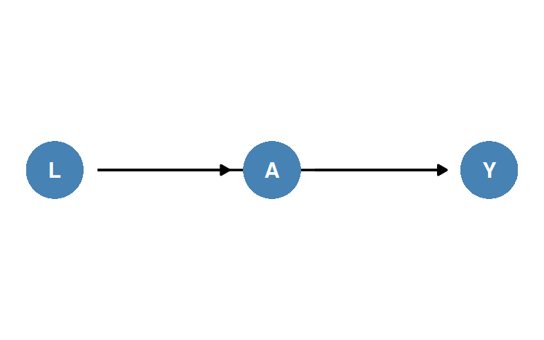
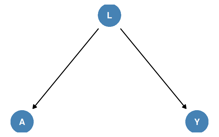
Example 1 (Markov Factorization Implies an Independence) Take the DAG \(A \leftarrow L \to Y\) (Figure 3). The parents are: none for \(L\); \(L\) for \(A\); \(L\) for \(Y\). Start from the chain rule, which holds for any distribution, and apply the Markov factorization:

\[ \begin{aligned} f(l, a, y) &= f(l)\, f(a \mid l)\, f(y \mid l, a) && \text{(chain rule)} \\ &= f(l)\, f(a \mid l)\, f(y \mid l) && \text{(the only parent of } Y \text{ is } L\text{)}. \end{aligned} \]

Dividing both sides by \(f(l)\):

\[ \begin{aligned} f(a, y \mid l) &= \frac{f(l, a, y)}{f(l)} && \text{(definition of conditional density)} \\ &= f(a \mid l)\, f(y \mid l) && \text{(substitute the factorization)}, \end{aligned} \]

so \(A \perp\!\!\!\perp Y \mid L\): the missing arrow from \(A\) to \(Y\) implies a conditional independence.

Graphs and Counterfactuals

Each causal DAG has an underlying counterfactual model (Technical Points 6.2 and 6.3). That model justifies the intuitive graphical rules in this chapter, but conventional diagrams do not show the counterfactual variables.

Single World Intervention Graphs (SWIGs) (Richardson and Robins 2013) put counterfactuals on the graph; they are introduced in Chapter 7.

Causal diagrams encode both causation (our subject-matter knowledge) and the associations that the causal structure implies. That simultaneous representation is what makes them attractive (Hernán and Robins 2020, 77). The book’s treatment is informal, aiming at conceptual insight rather than rigor.

Technical Point 6.2: Nonparametric Structural Equation Models

A nonparametric structural equation model (NPSEM) for a DAG with ordered nodes \(V_1, \ldots, V_M\) assumes unobserved errors \(\epsilon_m\) and unknown deterministic functions \(f_m\) such that

• \(V_1 = f_1(\epsilon_1)\);
• the one-step-ahead counterfactual \(V_m^{pa_m}\), the value of \(V_m\) when its parents are set to \(pa_m\), equals \(f_m(pa_m, \epsilon_m)\).

Only the parents of \(V_m\) have a direct effect on it. Every variable can be intervened on, and all factual and counterfactual values are obtained recursively.

Example 2 (The NPSEM for Book Figure 6.1) The structural equations are \(L = f_L(\epsilon_L)\), \(A = f_A(L, \epsilon_A)\), \(Y = f_Y(L, A, \epsilon_Y)\). Setting \(A\) to \(a\) leaves \(L\) unchanged, because \(L\) is not a descendant of \(A\), so the counterfactual outcome is obtained by substituting \(a\) for \(A\): \(Y^a = f_Y(L, a, \epsilon_Y)\).

Robins (1986) introduced this model as a finest causally interpreted structural tree graph (FCISTG) “as detailed as the data”; Pearl (2009) showed how to represent it with a DAG (Hernán and Robins 2020, Technical Point 6.2, p. 77). For exposition the book assumes every variable can be intervened on, although its statistical methods do not require this.

Technical Point 6.3: Which Independences?

An FCISTG alone does not imply the causal Markov assumption; independence assumptions must be added.

Model	Assumption	Fig. 6.2 implies
NPSEM-IE (Pearl)	all errors \(\epsilon_m\) mutually independent	full exchangeability \((Y^{a=0}, Y^{a=1}) \perp\!\!\!\perp A\)
FFRCISTG (Robins 1986)	one-step-ahead counterfactuals jointly independent	marginal exchangeability \(Y^a \perp\!\!\!\perp A\) for each \(a\)

Both imply the causal Markov assumption. An NPSEM-IE is an FFRCISTG, not vice versa. Unless stated otherwise, the book’s causal DAGs represent an FFRCISTG.

Source: Hernán and Robins (2020, Technical Point 6.3, p. 78). Robins and Richardson (2010) showed that Robins’s original formulation is equivalent to the joint-independence assumption for a positive distribution, and that an NPSEM-IE makes many more independence assumptions than an FFRCISTG.

2 6.2 Causal Diagrams and Marginal Independence (pp. 77-79)

Three examples, all with no conditioning:

Figure 3: Book Figure 6.3: smoking \(L\) causes carrying a lighter \(A\) and lung cancer \(Y\).

Figure 4: Book Figure 6.4: haplotype \(A\) and smoking \(Y\) both cause heart disease \(L\), a collider.

Figure	Structure	Example	\(A\) and \(Y\)
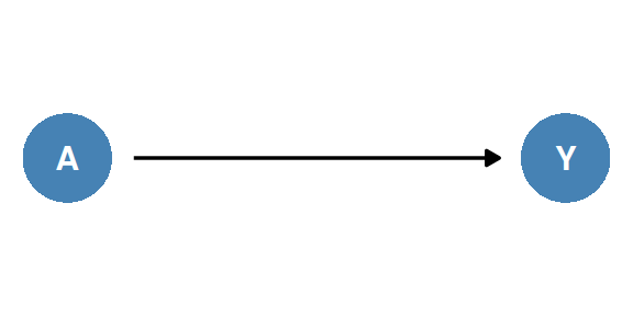
Figure 2	\(A \to Y\)	aspirin prevents heart disease (randomized)	associated
Figure 3	\(A \leftarrow L \to Y\)	lighter, smoking, lung cancer	associated (no effect of \(A\))
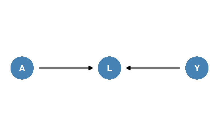
Figure 4	\(A \to L \leftarrow Y\)	haplotype, heart disease, smoking	independent

Paths and the Flow of Association

Definition 2 (Path; Causal Path) A path between \(R\) and \(S\) is a route connecting them along a sequence of edges that visits no variable more than once. A path is causal if all its arrows point in the same direction; otherwise it is noncausal (Hernán and Robins 2020, 78, margin note).

Picture paths as pipes through which association flows. Association is symmetric, so it flows regardless of the direction of the arrows.

Definition 3 (Collider) A variable on a path is a collider on that path if two arrowheads on the path collide at it, as \(L\) does on \(A \to L \leftarrow Y\).

The Three Examples

• Figure 2: causation implies association; in an ideal randomized experiment \(\Pr[Y^{a=1}=1] \neq \Pr[Y^{a=0}=1]\) if and only if \(\Pr[Y=1 \mid A=1] \neq \Pr[Y=1 \mid A=0]\).
• Figure 3: learning that Hera carries a lighter makes it likelier she smokes, hence likelier she gets lung cancer; association flows through the common cause \(L\), though \(A\) has no effect on \(Y\).
• Figure 4: learning that Apollo lacks the haplotype says nothing about his smoking; a collider blocks the flow of association, so \(A \perp\!\!\!\perp Y\).

Summary: two variables are marginally associated if one causes the other or if they share a common cause; otherwise they are marginally independent.

In Figure 3, an investigator who concludes from the association that carrying a lighter causes lung cancer makes a mistake: information about \(A\) improves prediction of \(Y\) without \(A\) affecting \(Y\) (Hernán and Robins 2020, 79). In Figure 4, that both \(A\) and \(Y\) cause heart disease \(L\) is irrelevant to the marginal association between \(A\) and \(Y\).

3 6.3 Causal Diagrams and Conditional Independence (pp. 80-81)

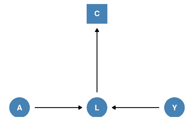
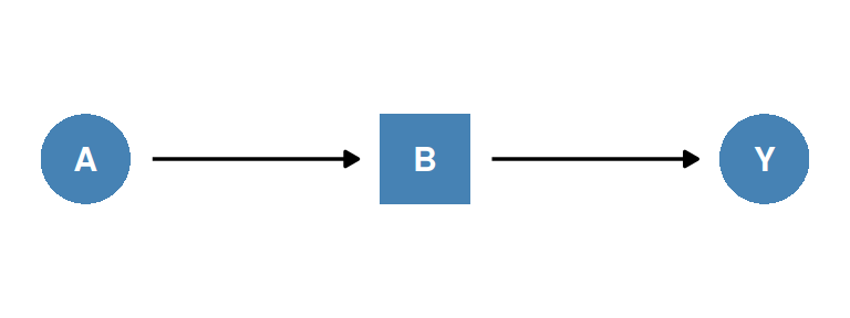
A square box around a node means we condition on it (e.g., restrict to one of its levels).

Figure 5: Book Figure 6.5: aspirin \(A\) lowers platelet aggregation \(B\), which affects heart disease \(Y\) (the square node \(B\) marks conditioning).

Structure	Conditioning on	Path	\(A\), \(Y\) given the conditioning variable
\(A \to B \to Y\) (Fig. 6.5)	mediator \(B\)	blocked	independent: \(A \perp\!\!\!\perp Y \mid B\)
\(A \leftarrow L \to Y\) (Fig. 6.6)	common cause \(L\)	blocked	independent: \(A \perp\!\!\!\perp Y \mid L\)
\(A \to L \leftarrow Y\) (Fig. 6.7)	collider \(L\)	opened	associated

• Mediator (Hernán and Robins 2020, 80): among those with low platelet aggregation (\(B=0\)), knowing whether someone took aspirin adds no information about heart disease, because aspirin acts only through \(B\): \(\Pr[Y=1 \mid A=1, B=b] = \Pr[Y=1 \mid A=0, B=b]\) for all \(b\).
• Common cause: among nonsmokers (\(L=0\)), carrying a lighter no longer predicts lung cancer. Blocking the flow of association through common causes is the graph-based justification for stratification as a way to achieve exchangeability.
• Because complete diagrams (all possible arrows present) imply no conditional independences, it is often said that the information about associations is in the missing arrows.

Conditioning on a Collider Opens the Path

In Figure 4, restrict to people with heart disease (\(L=1\), book Figure 6.7). Among them, someone without the haplotype is more likely to have the other cause, smoking: \(A\) and \(Y\) are inversely associated given \(L=1\).

In the extreme, if \(A\) and \(Y\) were the only causes of \(L\), then among those with \(L=1\) the absence of one would perfectly predict the presence of the other.

Intuition from the book (Hernán and Robins 2020, 81): whether two causes are associated cannot depend on a future event (their common effect), but two causes of an effect generally become associated once we stratify on that effect. Chapter 8 develops associations due to conditioning on common effects.

Conditioning on a Descendant of a Collider

Figure 6: Book Figure 6.8: diuretic use \(C\) follows a diagnosis of heart disease \(L\) (the square node \(C\) marks conditioning).

Conditioning on \(C\), a variable affected by the collider \(L\), also opens \(A \to L \leftarrow Y\). The path stays blocked only if we condition on neither \(L\) nor \(C\).

Three Structural Sources of Association

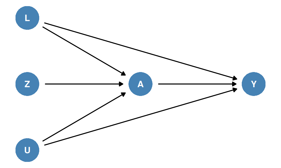
Two variables can be associated because

1. one causes the other;
2. they share a common cause;
3. they share a common effect and the analysis is restricted to a level of that effect (or of its descendants).

A fourth, nonstructural source is chance (random variability), which shrinks as the study population grows. Until Chapter 10 the book assumes a very large population, so all associations discussed are structural.

The heuristic arguments of this section are formalized by d-separation (Pearl 1995); Fine Point 6.1 lists the rules and Fine Point 6.2 introduces faithfulness (Hernán and Robins 2020, 81).

4 6.4 Positivity and Consistency in Causal Diagrams (pp. 81-85)

Fine Point 6.1: D-Separation

A path is blocked if and only if

• it contains a non-collider that has been conditioned on, or
• it contains a collider that has not been conditioned on and has no descendant that has been conditioned on.

Otherwise it is open. Two variables are d-separated if all paths between them are blocked; otherwise they are d-connected. Two sets are d-separated if each variable in one is d-separated from every variable in the other.

Example 3 (D-Separation in Book Figures 6.1 and 6.4)  

• Figure 1, \(A\) and \(L\): the path \(L \to A\) is open, so they are d-connected, even though the other path \(A \to Y \leftarrow L\) is blocked by the collider \(Y\).
• Figure 4, \(A\) and \(Y\): the only path is blocked by the collider \(L\), so they are d-separated.

From D-Separation to Independence

• Pearl (1988): under the causal Markov assumption, if \(\mathcal{A}\) is d-separated from \(\mathcal{B}\) given \(\mathcal{C}\), then \(\mathcal{A}\) is statistically independent of \(\mathcal{B}\) given \(\mathcal{C}\) (disjoint sets of variables).
• Faithfulness is the separate assumption that the converse holds: independence implies d-separation.

“d-” stands for directional. An equivalent set of graphical rules, moralization, was developed by Lauritzen et al. (1990) (Hernán and Robins 2020, Fine Point 6.1, p. 82).

Fine Point 6.2: Faithfulness

An arrow \(A \to Y\) means \(A\) affects \(Y\) for at least one individual, yet the average causal effect and the association can still both be null, when effects in different individuals cancel exactly. Such exact cancellation is rare, so the book assumes faithfulness: lack of d-separation can almost always be equated with a non-zero association.

Example 4 (Unfaithfulness from Cancelling Effects) In the book’s Table 4.1, transplant increases the risk of death in women and decreases it in men, each half of the population, and the effects cancel exactly: \(\Pr[Y^{a=1}=1] = \Pr[Y^{a=0}=1]\). Figure 2 is still the correct diagram, because \(A\) affects every individual’s \(Y\), but the expected association is absent: the distribution is not faithful to the DAG (Hernán and Robins 2020, Fine Point 6.2, p. 83).

Faithfulness can be violated by design. In a matched study (book Section 4.5, Figure 6.9), selection \(S\) depends on both \(A\) and \(L\), and the analysis is restricted to \(S=1\). D-separation predicts \(L\) and \(A\) associated given \(S\) (open paths \(L \to A\) and \(L \to S \leftarrow A\)), but matching makes them unassociated: the association created through \(L \to S \leftarrow A\) exactly cancels the one through \(L \to A\).

Faithfulness may also fail when variables are linked by deterministic arrows: two variables can then be independent even though some paths between them are open.

Graphs, Do-Calculus, and Notation

Standardization and IP weighting (Chapter 2) can also be derived from causal graph theory, as part of what is sometimes called the do-calculus (reviewed in Pearl 2009). So using counterfactuals in Chapters 1-5 privileged a notation, not an approach.

Whatever the notation, causal inference via standardization or IP weighting requires exchangeability, positivity, and consistency. This section covers positivity and consistency; exchangeability is translated into graphs in Section 6.5 and Chapters 7-8.

Positivity and Consistency in the Graph

• Positivity concerns arrows into treatment nodes. Causal graphs generally cannot encode its violations, except special cases, e.g., \(A\) a deterministic function of a pretreatment \(L\) (drawn as a bold \(L \to A\) arrow).
• Consistency (well-defined counterfactuals) concerns arrows out of treatment nodes: \(A \to Y\) must correspond to a possibly hypothetical but relatively unambiguous intervention (or, if \(A\) is a state, to well-defined interventions that affect \(Y\) only through \(A\); Fine Point 6.4).

In the book’s diagrams, positivity is implicit unless stated and consistency is embedded in the notation.

Treatment nodes thus have a special status (Hernán and Robins 2020, 83–84). Some authors draw it explicitly with decision nodes; influence diagrams are causal diagrams augmented with decision nodes (Dawid 2000, 2002). The book omits them, because it is always explicit about the interventions on \(A\), but gives treatment nodes a distinct status in SWIGs later. The causal trees of Chapter 2 and the sufficient-cause “pies” of Chapter 5 also distinguished treatments from other variables.

Treatment Nodes Need Well-Defined Interventions

Diagrams read as NPSEMs with independent errors seem to give all variables equal status, which can mislead when some nodes correspond to ill-defined interventions.

• A node for “obesity” may be acceptable as an outcome \(Y\) or a covariate \(L\).
• It is generally not acceptable as a treatment \(A\) (Chapter 3).

Pearl (2018, 2019) has proposed a concept of causation based on variables that “listen to others”, which still assumes well-defined counterfactuals for every variable (Hernán and Robins 2020, 84, margin note).

Figure 7: Book Figure 6.10, as described in the text: caloric intake \(Z\), exercise \(L\), and genetic traits \(U\) affect weight loss \(A\); \(L\) and \(U\) also affect mortality \(Y\) through other pathways.

When there are several ways to intervene on \(A\) and some of them affect \(Y\) directly, “the effect of \(A\) on \(Y\)” is unclear: losing weight by caloric restriction, by exercise, or by genetic manipulation would lead to different mortality. Being explicit about the intervention is a step toward a well-defined effect, relevant data, and the right adjustment variables.

Fine Point 6.3: Discovery of Causal Structure

Discovery is learning parts of the causal structure from data. It sometimes works if we assume faithfulness, but often it does not: a strong association between \(B\) and \(C\) fits \(B \to C\), \(C \to B\), a shared unmeasured cause, a conditioned-on common effect, and combinations.

Example 5 (Learning \(Z \to A \to Y\) (Hernán and Robins 2020, Fine Point 6.3, p. 85)) Suppose \(Z\) precedes \(A\), which precedes \(Y\), and with infinite data all three are marginally associated and the only conditional independence is \(Z \perp\!\!\!\perp Y \mid A\). Under faithfulness the only consistent causal DAGs are \(Z \to A \to Y\), possibly with a common cause of \(Z\) and \(A\) in addition to, or instead of, \(Z \to A\). Then there is no unmeasured common cause of \(A\) and \(Y\), and the average causal effect is identified by \(\operatorname{E}\mathopen{}\left[Y \mid A=1\right]\mathclose{} - \operatorname{E}\mathopen{}\left[Y \mid A=0\right]\mathclose{}\).

Why: a direct arrow \(Z \to Y\), a common cause of \(Z\) and \(Y\), or an unmeasured common cause of \(A\) and \(Y\) would each make \(Z\) and \(Y\) dependent given \(A\) (assuming faithfulness); the marginal association of \(A\) and \(Y\) then requires an arrow \(A \to Y\). If an unmeasured common cause of \(A\) and \(Y\) existed, no conditional independence would be found, and discovery could not tell whether \(A\) causes \(Y\). Approaches to discovery are described by Spirtes et al. (2000) and Peters et al. (2017); finite samples are discussed in the book’s Technical Point 10.7.

5 6.5 A Structural Classification of Bias (pp. 85-87)

Definition 4 (Systematic Bias) There is systematic bias when the data are insufficient to identify the causal effect even with an infinite sample size. Informally: any structural association between treatment and outcome that does not arise from the causal effect of treatment on outcome (Hernán and Robins 2020, 85).

• Unconditional bias: \(\Pr[Y^{a=1}=1] - \Pr[Y^{a=0}=1] \neq \Pr[Y=1 \mid A=1] - \Pr[Y=1 \mid A=0]\), the case when \(Y^a \perp\!\!\!\perp A\) fails.
• Conditional bias: \(\Pr[Y^{a=1}=1 \mid L=l] - \Pr[Y^{a=0}=1 \mid L=l] \neq \Pr[Y=1 \mid L=l, A=1] - \Pr[Y=1 \mid L=l, A=0]\) for at least one \(l\), generally the case when \(Y^a \perp\!\!\!\perp A \mid L=l\) fails for some \(a\) and \(l\).

With systematic bias no estimator can be consistent (see Chapter 1 for consistent estimators). Absence of unconditional bias means the association measure in the population is a consistent estimate of the corresponding effect measure. In this chapter “bias” means systematic bias, because the sample size is assumed infinite.

Bias Under the Null

Lack of exchangeability causes bias even when treatment has no effect: bias under the null.

Example 6 (Table 3.1) In the book’s observational study of Table 3.1 the causal risk ratio was 1, whereas the associational risk ratio was 1.26 (Hernán and Robins 2020, 86).

Any structure that causes bias under the null also causes bias under the alternative (a non-null effect); the converse is false.

For example, conditioning on some variables may cause selection bias under the alternative but not under the null (Greenland 1977; Hernán 2017; see also Chapter 18) (Hernán and Robins 2020, 86, margin note).

Two Structures That Break Exchangeability

1. Common causes of treatment and outcome: what many epidemiologists call confounding (Chapter 7).
2. Conditioning on common effects: what many epidemiologists call selection bias under the null (Chapter 8).

A third source is measurement bias (information bias), from mismeasured treatment, outcome, or covariates; some types also cause bias under the null (Chapter 9). Random variability is a separate, nonstructural source (Chapter 10).

All three biases can arise in observational studies and in randomized experiments. Earlier chapters used idealized experiments (no loss to follow-up, full adherence, blinded assignment), but real experiments rarely look like that; the remaining chapters of Part I examine the boundary between experimenting and observing (Hernán and Robins 2020, 86–87).

6 6.6 The Structure of Effect Modification (pp. 87-89)

Causal diagrams are good at locating sources of bias, but less helpful for illustrating effect modification.

Figure 8: Book Figure 6.12: randomized transplant \(A\); quality of care \(V\) affects death \(Y\).

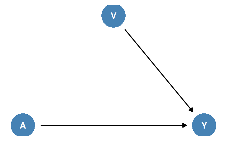
Transplant \(A\) is randomized, so association is causation; investigators stratify by quality of care \(V\) and find additive effect modification.

Two Caveats

1. Figure 8 would be valid without \(V\), since \(V\) is not a common cause of \(A\) and \(Y\); \(V\) appears only because the question refers to it. Variables on the path from \(V\) to \(Y\), such as therapy complications \(N\) (book Figure 6.13), could also be effect modifiers.
2. Figure 8 does not show whether, or how, \(V\) modifies the effect of \(A\). It cannot distinguish:
   • effects in the same direction in both strata of \(V\);
   • effects in opposite directions (qualitative effect modification);
   • an effect in one stratum only (e.g., \(A\) kills only those with \(V=0\)).

Surrogate Effect Modifiers

A surrogate effect modifier is associated with the causal effect modifier \(V\) but does not affect \(Y\). The association can come from any structure:

Book figure	Surrogate	Structure linking it to \(V\)
6.14	cost of treatment \(S\)	cause and effect: \(V \to S\)
6.15	passport nationality \(P\)	common cause: residence \(U\) affects \(V\) and \(P\)
6.16	bottled mineral water \(W\)	conditioning on a common effect: \(V\) and \(W\) affect cost \(S\), analysis restricted to \(S=0\)

Causal and surrogate effect modifiers are often indistinguishable in practice, so “effect modification” covers both (Section 4.2); some prefer the neutral term “heterogeneity of causal effects”. Reading “cost modifies the effect of transplant” causally could suggest raising prices without raising quality (Hernán and Robins 2020, 88).

Intuition for the mineral-water example (book margin note, p. 88): low-cost hospitals that buy mineral water must spend less on care that lowers mortality, so among low-cost hospitals, mineral water use is inversely associated with quality of care. VanderWeele and Robins (2007b) give a finer classification of effect modification via causal diagrams.

Interaction in Causal Diagrams

Causal diagrams are agnostic about interaction between two treatments \(A\) and \(E\). They can encode it if augmented with nodes for sufficient-component causes (Chapter 5), with deterministic arrows from the treatments to those nodes; the book develops such diagrams in Chapter 8.

Fine Point 6.4: Evidence That a State Has Well-Defined Counterfactuals

Consider drug \(Z\), systolic blood pressure \(A\) (a state, not directly manipulable), and stroke \(Y\). If (i) \(Z\) is associated with \(A\) and \(Y\), (ii) \(A\) and \(Y\) are associated, and (iii) \(Z \perp\!\!\!\perp Y \mid A\), then under faithfulness the only causal DAG has \(A \to Y\), no \(Z \to Y\), and no unmeasured common cause of \(A\) and \(Y\) or of \(Z\) and \(Y\) (the discovery argument of Fine Point 6.3).

• If \(Y^a\) is well defined, \(Y^a \perp\!\!\!\perp A\) holds and \(\operatorname{E}\mathopen{}\left[Y \mid A=1\right]\mathclose{} - \operatorname{E}\mathopen{}\left[Y \mid A=0\right]\mathclose{}\) is the average causal effect.
• An investigator who doubted that \(Y^a\) was well defined might take (i)-(iii) as empirical evidence that it is.

Usually unmeasured common causes \(U_3\) of \(A\) and \(Y\) remain; then \(Z\) and \(Y\) are associated given the collider \(A\), (iii) fails, and the data give no support for \(Y^a\) being well defined (Hernán and Robins 2020, Fine Point 6.4, p. 89).

The book’s remedy is a four-arm factorial dose-finding trial: randomize the drug (\(Z=1\) or \(Z=2\)) and the target blood-pressure reduction (\(A=a_1\) or \(A=a_2\)), and increase each individual’s dose \(D\) until the assigned reduction is reached and maintained. The achieved \(A\) is then a deterministic function of the assigned value, so nothing else has an arrow into \(A\) (book Figure 6.18). If \(Y\) is independent of \(D\) given \(A\) and \(\operatorname{E}\mathopen{}\left[Y \mid A=a_1\right]\mathclose{} \neq \operatorname{E}\mathopen{}\left[Y \mid A=a_2\right]\mathclose{}\), then under faithfulness (and assuming \(Y^{d,a}\) and \(Y^a\) are well defined) \(D\) has no direct effect on \(Y\) outside \(A\), and \(\operatorname{E}\mathopen{}\left[Y^{a_1} - Y^{a_2}\right]\mathclose{}\) is identified by \(\operatorname{E}\mathopen{}\left[Y \mid A=a_1\right]\mathclose{} - \operatorname{E}\mathopen{}\left[Y \mid A=a_2\right]\mathclose{}\), even with unknown common causes of \(A\) and \(Y\). In a standard trial (book Figure 6.17), by contrast, \(Y\) and \(Z\) are associated given \(A\), so a direct effect of \(Z\) on \(Y\) cannot be ruled out.

7 Summary

• A causal DAG encodes qualitative causal knowledge: an arrow means a direct effect for at least one individual; a missing arrow means none for anyone; all common causes of variables on the graph must be on the graph (causal Markov assumption).
• Each causal DAG represents a counterfactual model (by default an FFRCISTG).
• Association flows along open paths: marginally, causal chains and common causes transmit association, colliders block it; conditioning on a non-collider blocks a path, conditioning on a collider or its descendant opens it (d-separation).
• Faithfulness, assumed throughout the book, lets us equate d-connection with association.
• Graphs rarely show positivity violations; consistency requires treatment nodes with well-defined interventions.
• Systematic bias from lack of exchangeability has two structures: common causes (confounding) and conditioning on common effects (selection bias); measurement bias is a third type.
• Causal diagrams do not show whether or how a variable modifies an effect, and cannot separate causal from surrogate effect modifiers.

Looking ahead: Chapter 7 (confounding), Chapter 8 (selection bias), Chapter 9 (measurement bias), Chapter 10 (random variability).

The diagrams in this chapter are drawn with the R packages dagitty and ggdag.

8 References

Hernán, Miguel A, and James M Robins. 2020. Causal Inference: What If. Chapman & Hall/CRC. https://miguelhernan.org/whatifbook.