Nonparametric Models

Last modified: 2026-11-07 21:34:29 (PST)

1 Empirical distribution

Definition 1 (Empirical distribution) For observed values \(x_1, \ldots, x_n\), the empirical distribution is the distribution of a value chosen at random from the sample, each of the \(n\) observations being equally likely: the probability that the value falls in a set \(A\) is

\[\frac{1}{n}\sum_{j=1}^n{\mathbb{1}\mathopen{}\left(x_j \in A\right)\mathclose{}}.\]

Source: Wikipedia contributors [1].

Example 1 (Numerical example: empirical distribution) Suppose the observed values are \(4, 1, 7, 3\), so \(n = 4\), and let \(A = [2, 5)\). Two of the four values (4 and 3) lie in \(A\), so the empirical distribution gives \(A\) probability \(2/4 = 0.5\). Each observed value has probability \(1/4\), and any set containing none of them has probability \(0\).

2 Empirical CDF

Definition 2 (Empirical CDF) For observed values \(x_1, \ldots, x_n\), the empirical cumulative distribution function (empirical CDF) is the CDF of the empirical distribution, the function

\[{\mathop{\hat{\mathbb{F}}}\nolimits\mathopen{}\left(t\right)\mathclose{}} \stackrel{\text{def}}{=}\frac{1}{n}\sum_{j=1}^nI(x_j \le t), \quad t \in \mathbb{R},\]

where \(I(A)\) is the indicator function: \(I(A) = 1\) if \(A\) holds, and \(I(A) = 0\) otherwise.

Source: Wikipedia contributors [4].

Example 2 (Numerical example: empirical CDF) Suppose the observed values are \(4, 1, 7, 3\), so \(n = 4\). Two of the four values (1 and 3) are at most 3.5, so:

\[ \begin{aligned} \hat F(3.5) &= \frac{1}{4}\mathopen{}\left(I(4 \le 3.5) + I(1 \le 3.5) + I(7 \le 3.5) + I(3 \le 3.5)\right)\mathclose{} && \text{(definition of $\hat F$)}\\ &= \frac{1}{4}(0 + 1 + 0 + 1) && \text{(evaluate each indicator)}\\ &= 0.5 && \text{(arithmetic)} \end{aligned} \]

Similarly, \(\hat F(0) = 0\), because no value is at most 0, and \(\hat F(7) = 1\), because every value is at most 7.

Rice [5, Sec. 10.2.1], pp. 378–379 covers the empirical CDF.

3 Order statistics

Definition 3 (Order statistics) For observed values \(x_1, \ldots, x_n\), the order statistics are the same values sorted in increasing order, written

\[x_{(1)} \le x_{(2)} \le \cdots \le x_{(n)}.\]

So \(x_{(1)}\) is the smallest value and \(x_{(n)}\) is the largest.

Source: Wikipedia contributors [6].

Example 3 (Numerical example: order statistics) If the observed values are \(4, 1, 7, 3\), then the order statistics are \(x_{(1)} = 1\), \(x_{(2)} = 3\), \(x_{(3)} = 4\), and \(x_{(4)} = 7\).

  • Hogg et al. [7, Sec. 6.3], pp. 256–263 covers order statistics.
  • Casella and Berger [8, Sec. 5.4], pp. 226–231 covers order statistics.

4 Sample quantiles

Definition 4 (Sample quantile function (empirical quantile function)) Given an empirical CDF \(\hat F\), the sample quantile function (also called the empirical quantile function) is

\[\hat Q(p) \stackrel{\text{def}}{=}\inf\mathopen{}\left\{t : \hat F(t) \ge p\right\}\mathclose{}, \quad 0 < p \le 1.\]

Source: Wikipedia contributors [9].

Definition 5 (Sample \(p\) quantile (sample \(100p\)th percentile)) For a given \(p\), the value \(\hat Q(p)\) of the sample quantile function is the sample \(p\) quantile, also called the sample \(100p\)th percentile.

The CDF \(F\) and the quantile function \(Q\) describe a probability distribution, while \(\hat F\) and \(\hat Q\) describe a sample, and serve as estimates of \(F\) and \(Q\).

Theorem 1 (Order-statistics form of the sample quantile) If \(x_{(1)} \le \cdots \le x_{(n)}\) are the order statistics and \(i \in \mathopen{}\left\{1, \ldots, n\right\}\mathclose{}\), then \(\hat Q(p) = x_{(i)}\) for every \(p\) with \((i-1)/n < p \le i/n\). In particular, \(\hat Q(i/n) = x_{(i)}\).

Proof. Let \(p\) satisfy \((i-1)/n < p \le i/n\).

For any \(t < x_{(i)}\), the \(n - i + 1\) values \(x_{(i)}, \ldots, x_{(n)}\) all exceed \(t\), so at most \(i - 1\) values are at most \(t\), and:

\[ \begin{aligned} \hat F(t) &\le \frac{i-1}{n} && \text{(at most $i - 1$ indicators equal 1)}\\ &< p && \text{(choice of $p$)} \end{aligned} \]

So no \(t < x_{(i)}\) belongs to the set \(\mathopen{}\left\{t : \hat F(t) \ge p\right\}\mathclose{}\).

At \(t = x_{(i)}\), the \(i\) values \(x_{(1)}, \ldots, x_{(i)}\) are all at most \(x_{(i)}\), so:

\[ \begin{aligned} \hat F\mathopen{}\left(x_{(i)}\right)\mathclose{} &\ge \frac{i}{n} && \text{(at least $i$ indicators equal 1)}\\ &\ge p && \text{(choice of $p$)} \end{aligned} \]

So \(x_{(i)}\) belongs to the set, and it is the smallest member of the set, because no smaller \(t\) belongs to it. Therefore \(\hat Q(p) = x_{(i)}\).

Example 4 (Numerical example: sample quantiles) Using the same data \(4, 1, 7, 3\), with order statistics \(1, 3, 4, 7\), Theorem 1 says the sample quantile function is a step function:

  • \(\hat Q(p) = 1\) for \(0 < p \le 1/4\);
  • \(\hat Q(p) = 3\) for \(1/4 < p \le 1/2\);
  • \(\hat Q(p) = 4\) for \(1/2 < p \le 3/4\);
  • \(\hat Q(p) = 7\) for \(3/4 < p \le 1\).

So \(\hat Q(0.5) = 3\) and \(\hat Q(0.9) = 7\). R’s quantile() function computes this definition when called with type = 1:

quantile(c(4, 1, 7, 3), probs = c(0.5, 0.9), type = 1)
#> 50% 90% 
#>   3   7

Remark 1 (Quantile conventions). Other sources, and other software defaults, define sample quantiles differently, mostly by interpolating between order statistics. R’s quantile() offers nine definitions through its type argument, and its default (type = 7) interpolates, so quantile(c(4, 1, 7, 3), 0.5) returns 3.5, not 3. The usual sample median is another interpolated quantile: for an even number of observations, it averages the two middle order statistics. These notes use Definition 4, which always returns one of the observed values.

Hogg et al. [7, Sec. 7.5], pp. 337–343 covers distribution-free confidence intervals for percentiles.

5 The empirical CDF and quantile function as generalized inverses

Figure 1: The empirical CDF and the sample quantile function for the data 4, 1, 7, 3 (order statistics 1, 3, 4, 7).
[Code]
x <- c(4, 1, 7, 3)
n <- length(x)
x_ord <- sort(x)
p_ord <- seq_len(n) / n
ecdf_x_padding <- 0.8
x_min <- min(x_ord) - ecdf_x_padding
x_max <- max(x_ord) + ecdf_x_padding

x_left <- c(x_min, x_ord)
x_right <- c(x_ord, x_max)
f_levels <- c(0, p_ord)

ecdf_pieces <- tibble::tibble(x = x_left, xend = x_right, y = f_levels)
ecdf_open <- tibble::tibble(x = x_ord, y = f_levels[seq_len(n)])
ecdf_closed <- tibble::tibble(x = x_ord, y = f_levels[seq_len(n) + 1])

ggplot2::ggplot() +
  ggplot2::geom_segment(
    ggplot2::aes(x = x, xend = xend, y = y, yend = y),
    data = ecdf_pieces, linewidth = 1, color = "blue"
  ) +
  ggplot2::geom_point(
    ggplot2::aes(x = x, y = y), data = ecdf_open, shape = 1, color = "blue"
  ) +
  ggplot2::geom_point(
    ggplot2::aes(x = x, y = y), data = ecdf_closed, shape = 19, color = "blue"
  ) +
  ggplot2::coord_cartesian(xlim = c(x_min, x_max), ylim = c(0, 1.05)) +
  ggplot2::labs(
    x = "Value, t",
    y = expression("Empirical CDF, " * hat(plain("F"))(t))
  ) +
  ggplot2::theme_minimal()
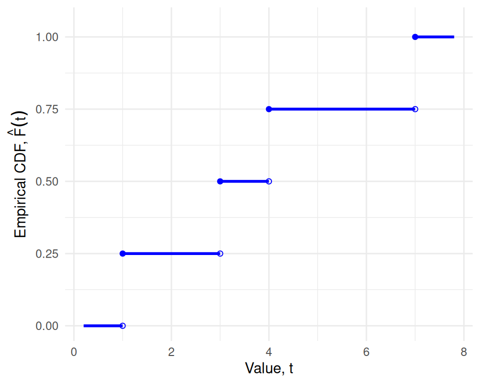
(a) Empirical CDF, horizontal pieces only. Closed circles mark included endpoints; open circles mark excluded endpoints.

[Code]
eqf_y_padding <- 0.5
q_left <- c(0, p_ord[-n])
q_right <- p_ord
eqf_pieces <- tibble::tibble(x = q_left, xend = q_right, y = x_ord)

ggplot2::ggplot(eqf_pieces) +
  ggplot2::geom_segment(
    ggplot2::aes(x = x, xend = xend, y = y, yend = y),
    linewidth = 1, color = "blue"
  ) +
  ggplot2::geom_point(ggplot2::aes(x = x, y = y), shape = 1, color = "blue") +
  ggplot2::geom_point(
    ggplot2::aes(x = xend, y = y), shape = 19, color = "blue"
  ) +
  ggplot2::coord_cartesian(
    xlim = c(0, 1),
    ylim = c(min(x_ord) - eqf_y_padding, max(x_ord) + eqf_y_padding)
  ) +
  ggplot2::labs(
    x = "Probability, p",
    y = expression("Sample quantile, " * hat(Q)(p))
  ) +
  ggplot2::theme_minimal()
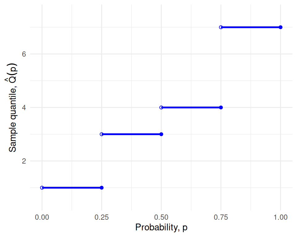
(b) Sample quantile function, horizontal pieces only. Open circles mark excluded left endpoints; closed circles mark included right endpoints.

Both functions in Figure 1 are step functions, so neither is one-to-one. Each flat piece of one function corresponds to a jump of the other: for example, \(\hat F(t) = 0.5\) for every \(t \in [3, 4)\), and \(\hat Q\) jumps from 3 to 4 at \(p = 0.5\). So \(\hat Q\) is a generalized inverse of \(\hat F\), not an inverse in the usual sense: \(\hat Q(\hat F(t)) \le t\) for every \(t \ge x_{(1)}\), with equality only at the observed values.

These readings look ahead from the empirical CDF to distribution-free tests, which this page does not cover:

References

[1]
Wikipedia contributors, “Empirical measure — Wikipedia, the free encyclopedia.” 2026. Available: https://en.wikipedia.org/wiki/Empirical_measure
[2]
T. Hastie, R. Tibshirani, and J. Friedman, The elements of statistical learning: Data mining, inference, and prediction, 2nd ed. Springer, 2009. doi: 10.1007/978-0-387-84858-7.
[3]
B. Efron and R. J. Tibshirani, An introduction to the bootstrap. in Monographs on statistics and applied probability, no. 57. New York: Chapman & Hall/CRC, 1993. doi: 10.1201/9780429246593.
[4]
Wikipedia contributors, “Empirical distribution function — Wikipedia, the free encyclopedia.” 2026. Available: https://en.wikipedia.org/wiki/Empirical_distribution_function
[5]
J. A. Rice, Mathematical statistics and data analysis, 3rd ed. Belmont, CA: Cengage Learning, 2007.
[6]
Wikipedia contributors, “Order statistic — Wikipedia, the free encyclopedia.” 2026. Available: https://en.wikipedia.org/wiki/Order_statistic
[7]
R. V. Hogg, E. A. Tanis, and D. L. Zimmerman, Probability and statistical inference, Tenth edition. Boston: Pearson, 2019.
[8]
G. Casella and R. Berger, Statistical inference, 2nd ed. Cengage Learning, 2002. Available: https://www.cengage.com/c/statistical-inference-2e-casella-berger/9780534243128/
[9]
Wikipedia contributors, “Quantile — Wikipedia, the free encyclopedia.” 2026. Available: https://en.wikipedia.org/wiki/Quantile