Key distributions

Last modified: 2026-09-28 23:45:35 (PDT)

Remark. Some distributions are typically used for outcome models (Table 1); other distributions are typically used for test statistics (Table 2).

Table 1: Distributions typically used for outcome models

Distribution	Uses
Bernoulli	Binary outcomes
Binomial	Sums of Bernoulli outcomes
Poisson	Unbounded count outcomes
Geometric	Counts of non-events before an event occurs
Negative binomial	Mixtures of Poisson distributions, counts of non-events until a given number of events occurs
Normal (Gaussian)	Continuous outcomes without a more specific distribution
Multivariate normal	Vectors of continuous outcomes
Mixtures	Outcomes from a population of unobserved subpopulations
Exponential	Time to event outcomes
Gamma	Time to event outcomes
Weibull	Time to event outcomes
Log-normal	Time to event outcomes

Table 2: Distributions typically used for test statistics

Distribution	Uses
\(\chi^2\)	Regression comparisons (asymptotic), contingency table independence tests, goodness-of-fit tests
\(F\)	Gaussian model comparisons (exact)
\(Z\) (standard normal)	Proportions, means, regression coefficients (asymptotic)
\(t\) (Student’s)	Means, regression coefficients in Gaussian outcome models (exact)

1 The Bernoulli distribution

Example 1 (A coin flip) The Bernoulli distribution describes a binary outcome. The indicator of heads on one flip of a fair coin is \(\operatorname{Ber}(1/2)\). By the expectation of the Bernoulli distribution, \(X \sim \operatorname{Ber}(\pi)\) has mean \(\pi\), and by the variance of a Bernoulli random variable, it has variance \(\pi(1 - \pi)\).

2 The Poisson distribution

Definition 1 (Poisson distribution) A random variable \(Y\) has the Poisson distribution with mean parameter \(\mu > 0\), written \(Y \sim \operatorname{Pois}(\mu)\), if:

\[\operatorname{P}(Y = y) \stackrel{\text{def}}{=}\frac{\mu^{y} e^{-\mu}}{y!}, \quad y \in \mathbb{N}= \mathopen{}\left\{0, 1, 2, \dots\right\}\mathclose{} \tag{1}\]

Remark. (see Figure 1)

Exercise 1 What is the range of possible values for a Poisson distribution?

Solution 1. \[\mathcal{R}(Y) = \mathopen{}\left\{0, 1, 2, \dots\right\}\mathclose{} = \mathbb{N}\]

Theorem 1 (CDF of Poisson distribution) If \(Y \sim \operatorname{Pois}(\mu)\), then for every real number \(y\):

\[\operatorname{P}(Y \le y) = e^{-\mu} \sum_{j=0}^{\mathopen{}\left\lfloor y\right\rfloor\mathclose{}}\frac{\mu^j}{j!} \tag{2}\]

Proof. For \(y < 0\), both sides are \(0\) (the sum is empty). For any \(y \ge 0\), the event \(\{Y \le y\}\) is the disjoint union of events \(\{Y = j\}\) for all non-negative integers \(j \le \mathopen{}\left\lfloor y\right\rfloor\mathclose{}\). Applying the Poisson PMF (Equation 1) and factoring out the common term \(e^{-\mu}\):

\[ \begin{aligned} \operatorname{P}(Y \le y) &= \sum_{j=0}^{\mathopen{}\left\lfloor y\right\rfloor\mathclose{}} \operatorname{P}(Y = j) && (\text{disjoint union of events } Y = j) \\ &= \sum_{j=0}^{\mathopen{}\left\lfloor y\right\rfloor\mathclose{}} \frac{\mu^j e^{-\mu}}{j!} && (\text{definition of Poisson PMF}) \\ &= e^{-\mu} \sum_{j=0}^{\mathopen{}\left\lfloor y\right\rfloor\mathclose{}} \frac{\mu^j}{j!} && (\text{factoring out } e^{-\mu} \text{ constant wrt } j) \end{aligned} \]

Example 2 (Computing Poisson cumulative probabilities) For a Poisson random variable \(X \sim \operatorname{Pois}(\mu = 2)\), the probability of observing at most 2 events is computed as:

\[ \begin{aligned} \operatorname{P}(X \le 2) &= e^{-2} \sum_{j=0}^{2} \frac{2^j}{j!} && (\text{apply CDF formula with } \mu = 2, y = 2) \\ &= e^{-2} \mathopen{}\left(\frac{2^0}{0!} + \frac{2^1}{1!} + \frac{2^2}{2!}\right)\mathclose{} && (\text{expand terms for } j = 0, 1, 2) \\ &= e^{-2} \mathopen{}\left(1 + 2 + 2\right)\mathclose{} && (\text{simplify factorials and powers}) \\ &= 5 e^{-2} \approx 0.677 && (\text{evaluate numerical value}) \end{aligned} \]

Remark. (see Figure 2)

pois_dists <-
  dplyr::tibble(mu = c(0.5, 1, 2, 5, 10, 20)) |>
  dplyr::reframe(.by = mu, x = 0:30) |>
  dplyr::mutate(
    `P(X = x)` = dpois(x, lambda = mu),
    `P(X <= x)` = ppois(x, lambda = mu),
    mu = factor(mu)
  )

plot0 <-
  pois_dists |>
  ggplot2::ggplot(
    ggplot2::aes(
      x = x,
      y = `P(X = x)`,
      fill = mu,
      col = mu
    )
  ) +
  ggplot2::theme(legend.position = "bottom") +
  ggplot2::labs(
    fill = latex2exp::TeX("$\\mu$"),
    col = latex2exp::TeX("$\\mu$"),
    y = latex2exp::TeX("$\\Pr_{\\mu}(X = x)$")
  )

plot1 <-
  plot0 +
  ggplot2::geom_segment(yend = 0) +
  ggplot2::facet_wrap(~mu)

print(plot1)

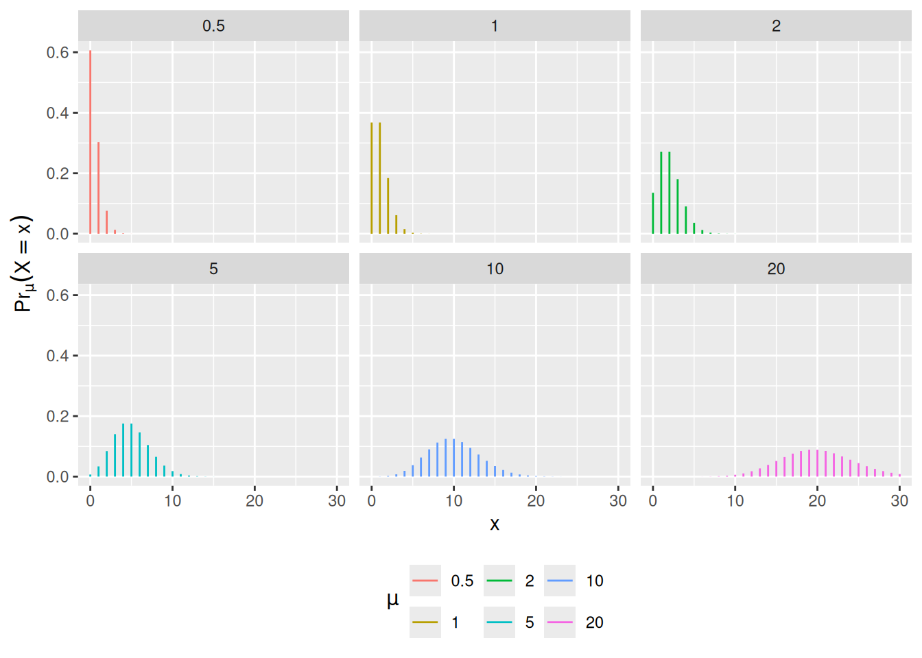
Figure 1: Poisson PMFs, by mean parameter \(\mu\)

plot2 <-
  plot0 +
  ggplot2::geom_step(alpha = 0.75) +
  ggplot2::aes(y = `P(X <= x)`) +
  ggplot2::labs(y = latex2exp::TeX("$\\Pr_{\\mu}(X \\leq x)$"))

print(plot2)

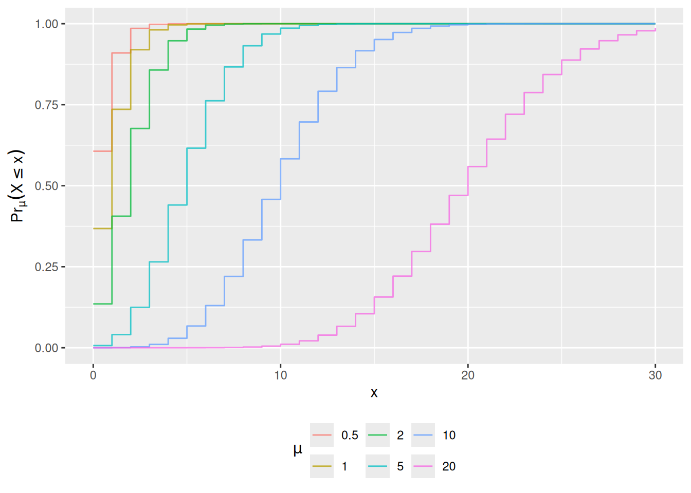
Figure 2: Poisson CDFs

Exercise 2 (Poisson distribution functions) Let \(X \sim \operatorname{Pois}(\mu = 3.75)\).

Compute:

• \(\operatorname{P}(X = 4)\)
• \(\operatorname{P}(X \le 7)\)
• \(\operatorname{P}(X > 5)\)

Solution.

• \(\operatorname{P}(X=4) = 0.1937803\)
• \(\operatorname{P}(X\le 7) = 0.9623787\)
• \(\operatorname{P}(X > 5) = 0.1771172\)

Theorem 2 (Properties of the Poisson distribution) If \(X \sim \operatorname{Pois}(\mu)\), then:

• \(\operatorname{E}[X] = \mu\)
• \(\operatorname{Var}(X) = \mu\)
• \(\operatorname{P}(X=x) = \frac{\mu}{x} \operatorname{P}(X = x-1)\) for \(x \in \mathopen{}\left\{1, 2, \dots\right\}\mathclose{}\)
• For \(x \in \mathopen{}\left\{1, 2, \dots\right\}\mathclose{}\) with \(x < \mu\), \(\operatorname{P}(X=x) > \operatorname{P}(X = x-1)\)
• For \(x = \mu\) (possible only when \(\mu\) is an integer), \(\operatorname{P}(X=x) = \operatorname{P}(X = x-1)\)
• For \(x \in \mathopen{}\left\{1, 2, \dots\right\}\mathclose{}\) with \(x > \mu\), \(\operatorname{P}(X=x) < \operatorname{P}(X = x-1)\)
• If \(\mu\) is not an integer, \(\arg \max_{x} \operatorname{P}(X=x) = \mathopen{}\left\lfloor\mu\right\rfloor\mathclose{}\); if \(\mu\) is an integer, the maximum is attained at both \(x = \mu - 1\) and \(x = \mu\)

Proof. Mean.

\[ \begin{aligned} \operatorname{E}[X] &= \sum_{x=0}^\infty x \cdot \operatorname{P}(X=x) && (\text{definition of expected value}) \\ &= 0 \cdot \operatorname{P}(X=0) + \sum_{x=1}^\infty x \cdot \operatorname{P}(X=x) && (\text{separate } x=0 \text{ term}) \\ &= \sum_{x=1}^\infty x \cdot \frac{\mu^x e^{-\mu}}{x!} && (\text{substitute Poisson PMF}) \\ &= \sum_{x=1}^\infty x \cdot \frac{\mu^x e^{-\mu}}{x \cdot (x-1)!} && (\text{definition of factorial } x!) \\ &= \sum_{x=1}^\infty \frac{\mu^x e^{-\mu}}{(x-1)!} && (\text{cancel factor of } x) \\ &= \mu \cdot \sum_{x=1}^\infty \frac{\mu^{x-1} e^{-\mu}}{(x-1)!} && (\text{factor out one power of } \mu) \\ &= \mu \cdot \sum_{y=0}^\infty \frac{\mu^y e^{-\mu}}{y!} && (\text{change index variable } y \stackrel{\text{def}}{=}x-1) \\ &= \mu \cdot 1 && (\text{PMF sums to 1 over state space}) \\ &= \mu && (\text{simplify}) \end{aligned} \]

Variance. The same steps, canceling two factors instead of one, give \(\operatorname{E}\mathopen{}\left[X(X-1)\right]\mathclose{}\):

\[ \begin{aligned} \operatorname{E}\mathopen{}\left[X(X-1)\right]\mathclose{} &= \sum_{x=2}^\infty x(x-1) \cdot \frac{\mu^x e^{-\mu}}{x!} && (\text{LOTUS; the } x = 0, 1 \text{ terms are } 0) \\ &= \sum_{x=2}^\infty \frac{\mu^x e^{-\mu}}{(x-2)!} && (\text{cancel } x(x-1) \text{ against } x!) \\ &= \mu^2 \cdot \sum_{y=0}^\infty \frac{\mu^y e^{-\mu}}{y!} && (\text{factor out } \mu^2 \text{; } y \stackrel{\text{def}}{=}x - 2) \\ &= \mu^2 && (\text{PMF sums to 1}) \end{aligned} \]

Then, by the simplified expression for variance and linearity of expectation:

\[ \begin{aligned} \operatorname{Var}(X) &= \operatorname{E}\mathopen{}\left[X^2\right]\mathclose{} - \mathopen{}\left(\operatorname{E}\mathopen{}\left[X\right]\mathclose{}\right)^2\mathclose{} && (\text{simplified expression for variance}) \\ &= \operatorname{E}\mathopen{}\left[X(X-1)\right]\mathclose{} + \operatorname{E}\mathopen{}\left[X\right]\mathclose{} - \mathopen{}\left(\operatorname{E}\mathopen{}\left[X\right]\mathclose{}\right)^2\mathclose{} && (X^2 = X(X-1) + X \text{; linearity}) \\ &= \mu^2 + \mu - \mu^2 && (\text{substitute}) \\ &= \mu && (\text{simplify}) \end{aligned} \]

Ratio of consecutive probabilities. For \(x \in \mathopen{}\left\{1, 2, \dots\right\}\mathclose{}\):

\[ \begin{aligned} \frac{\operatorname{P}(X = x)}{\operatorname{P}(X = x - 1)} &= \frac{\mu^x e^{-\mu} / x!}{\mu^{x-1} e^{-\mu} / (x-1)!} && (\text{substitute Poisson PMF}) \\ &= \frac{\mu}{x} && (\text{cancel } \mu^{x-1} e^{-\mu} \text{ and } (x-1)!) \end{aligned} \]

This ratio is greater than, equal to, or less than 1 as \(x\) is less than, equal to, or greater than \(\mu\), which gives the three comparisons. So \(\operatorname{P}(X = x)\) increases while \(x < \mu\) and decreases once \(x > \mu\). If \(\mu\) is not an integer, the last increase is at \(x = \mathopen{}\left\lfloor\mu\right\rfloor\mathclose{}\), which is therefore the unique mode. If \(\mu\) is an integer, \(\operatorname{P}(X = \mu) = \operatorname{P}(X = \mu - 1)\), and both are modes.

See also https://statproofbook.github.io/P/poiss-mean and https://statproofbook.github.io/P/poiss-var.

Example 3 (Mode of a Poisson distribution) For \(X \sim \operatorname{Pois}(2.5)\), \(\operatorname{P}(X = 2) = \frac{2.5}{2}\operatorname{P}(X = 1) > \operatorname{P}(X = 1)\) and \(\operatorname{P}(X = 3) = \frac{2.5}{3}\operatorname{P}(X = 2) < \operatorname{P}(X = 2)\), so the mode is \(\mathopen{}\left\lfloor 2.5\right\rfloor\mathclose{} = 2\). For \(X \sim \operatorname{Pois}(2)\), \(\operatorname{P}(X = 2) = \frac{2}{2}\operatorname{P}(X = 1)\), so \(1\) and \(2\) are both modes, each with probability \(2 e^{-2} \approx 0.271\).

Definition 2 (Exposure magnitude) For many count outcomes, there is some sense of an exposure magnitude, such as population size or duration of observation, which multiplicatively rescales the expected (mean) count.

Exercise 3 What are some examples of exposure magnitudes?

Solution.

Table 3: Examples of exposure units

outcome	exposure units
disease incidence	number of individuals exposed; time at risk
car accidents	miles driven
worksite accidents	person-hours worked
population size	size of habitat

Remark. Exposure units are similar to the number of trials in a binomial distribution, but in non-binomial count outcomes, there can be more than one event per unit of exposure.

We can use \(t\) to represent continuous-valued exposures/observation durations, and \(n\) to represent discrete-valued exposures.

Definition 3 (Event rate) For a count \(Y\) observed over a fixed, known exposure magnitude \(t > 0\), the event rate, denoted \(\lambda\), is the mean of \(Y\) divided by the exposure magnitude:

\[\lambda \stackrel{\text{def}}{=}\frac{\operatorname{E}\mathopen{}\left[Y\right]\mathclose{}}{t} \tag{3}\]

Remark. The event rate is a transformation of the mean: it removes the exposure magnitude from the mean, so counts observed over different exposures can be compared on one scale. Regression models for counts use the same decomposition, with the rate depending on covariates and the exposure magnitude known (see rme’s count-regression chapter).

Theorem 3 (Transformation function from event rate to mean) If a count \(Y\) is observed over exposure magnitude \(t > 0\) with event rate \(\lambda\), then its mean \(\mu \stackrel{\text{def}}{=}\operatorname{E}\mathopen{}\left[Y\right]\mathclose{}\) is:

\[\mu = \lambda \cdot t \tag{4}\]

Proof. By Definition 3:

\[ \begin{aligned} \lambda &\stackrel{\text{def}}{=}\frac{\operatorname{E}\mathopen{}\left[Y\right]\mathclose{}}{t} && (\text{definition of event rate}) \\ \operatorname{E}\mathopen{}\left[Y\right]\mathclose{} &= \lambda \cdot t && (\text{multiply both sides by } t > 0) \\ \mu &= \lambda \cdot t && (\mu \stackrel{\text{def}}{=}\operatorname{E}\mathopen{}\left[Y\right]\mathclose{}) \end{aligned} \]

Example 4 (Calculating expected counts from event rates) Suppose a city records a disease event rate of \(\lambda = 0.05\) cases per person-year. For a subpopulation with an exposure magnitude of \(t = 100\) person-years, the expected count of cases is, by Theorem 3:

\[ \begin{aligned} \mu &= \lambda \cdot t && (\text{transformation from event rate to mean}) \\ &= 0.05 \times 100 && (\text{substitute } \lambda = 0.05 \text{ and } t = 100) \\ &= 5 \text{ cases} && (\text{evaluate expected count}) \end{aligned} \]

Theorem 4 (No exposure means no expected events) For each exposure magnitude \(t \ge 0\), let \(Y_t\) be the count observed over exposure \(t\). If the mean count is proportional to the exposure magnitude, \(\operatorname{E}\mathopen{}\left[Y_t\right]\mathclose{} = \lambda \cdot t\) for all \(t \ge 0\) with one finite rate \(\lambda\), then there are no expected events without exposure:

\[\operatorname{E}\mathopen{}\left[Y_0\right]\mathclose{} = 0\]

Proof. \[ \begin{aligned} \operatorname{E}\mathopen{}\left[Y_0\right]\mathclose{} &= \lambda \cdot 0 && (\text{evaluate } \operatorname{E}\mathopen{}\left[Y_t\right]\mathclose{} = \lambda t \text{ at } t = 0) \\ &= 0 && (\text{multiplication by zero; } \lambda \text{ is finite}) \end{aligned} \]

Remark. The hypothesis carries the content here. Definition 3 alone cannot give \(\operatorname{E}\mathopen{}\left[Y_0\right]\mathclose{} = 0\), since \(\lambda = \operatorname{E}\mathopen{}\left[Y\right]\mathclose{}/t\) is undefined at \(t = 0\); the result holds for a model that assumes one rate \(\lambda\) shared across exposure magnitudes, including \(t = 0\).

Example 5 (Zero exposure time) If a subject is observed for \(t = 0\) person-years, no follow-up time has elapsed, so under a constant-rate model the expected number of incident events is \(\operatorname{E}\mathopen{}\left[Y_0\right]\mathclose{} = 0\).

Important

A mean proportional to exposure, \(\operatorname{E}\mathopen{}\left[Y_t\right]\mathclose{} = \lambda t\), has no term that stays nonzero at \(t = 0\): a model of this form says that with no exposure, no events are expected. A mean with an added constant, such as \(\operatorname{E}\mathopen{}\left[Y_t\right]\mathclose{} = c + \lambda t\) with \(c > 0\), would expect \(c\) events even with no exposure. Regression models for counts keep the proportional form when they add covariates (see rme’s count-regression chapter).

Theorem 5 (Exposure is additive on the log scale) If \(\mu = \lambda\cdot t\) with \(\lambda > 0\) and \(t > 0\), then:

\[\log{\mu} = \log{\lambda} + \log{t}\]

Proof. \[ \begin{aligned} \log{\mu} &= \log(\lambda \cdot t) && (\text{substitute } \mu = \lambda \cdot t) \\ &= \log{\lambda} + \log{t} && (\text{logarithm product rule}) \end{aligned} \]

Example 6 (Log-linear representation of expected counts) If a clinic sees an event rate of \(\lambda = 0.02\) events/day and \(t = 30\) days of observation:

\[ \begin{aligned} \log{\mu} &= \log(0.02) + \log(30) && (\text{apply log-scale formula}) \\ &= -3.912 + 3.401 && (\text{evaluate natural logarithms}) \\ &= -0.511 && (\text{sum terms}) \end{aligned} \]

Exponentiating yields \(\mu = \operatorname{exp}\mathopen{}\left\{-0.511\right\}\mathclose{} \approx 0.60\) expected events.

Definition 4 (Offset) For a count outcome with exposure magnitude \(t\), the known term \(\log{t}\) in the log-scale decomposition of the mean (Theorem 5),

\[\log{\mu} = \log{\lambda} + \log{t},\]

is called the offset: it shifts \(\log{\mu}\) by a known amount, with no unknown coefficient to estimate.

Remark. The offset needs no covariates: with a single exposure \(t\) and an unknown rate \(\lambda\), \(\log{t}\) is already an offset. Regression models for counts keep the same term and add covariate terms beside it (see rme’s count-regression chapter).

Example 7 (The offset for a clinic’s event count) In Example 6, the clinic was observed for \(t = 30\) days, so the offset is \(\log{30} \approx 3.401\). Only \(\log{\lambda}\) is unknown before the data are seen; the offset is fixed by the length of observation. A clinic observed for \(t = 60\) days has offset \(\log{60} \approx 4.094\), which raises \(\log{\mu}\) by \(\log{2} \approx 0.693\) at the same event rate.

Theorem 6 (Sum of independent Poisson random variables) If \(X\) and \(Y\) are independent Poisson random variables with means \(\mu_X\) and \(\mu_Y\), their sum, \(Z=X+Y\), is also a Poisson random variable, with mean \(\mu_Z = \mu_X + \mu_Y\).

Proof. The event \(\{Z = z\}\) is the disjoint union of the events \(\{X = k, Y = z - k\}\) for \(k = 0, 1, \ldots, z\) (since \(X\) and \(Y\) are non-negative integers), so:

\[ \begin{aligned} \operatorname{P}(Z = z) &= \sum_{k=0}^z \operatorname{P}(X = k,\, Y = z - k) && (\text{countable additivity}) \\ &= \sum_{k=0}^z \operatorname{P}(X = k) \operatorname{P}(Y = z - k) && (\text{independence}) \\ &= \sum_{k=0}^z \frac{\mu_X^k e^{-\mu_X}}{k!} \frac{\mu_Y^{z-k} e^{-\mu_Y}}{(z-k)!} && (\text{substitute Poisson PMFs}) \\ &= e^{-(\mu_X + \mu_Y)} \sum_{k=0}^z \frac{\mu_X^k \mu_Y^{z-k}}{k!(z-k)!} && (\text{factor out } e^{-\mu_X} e^{-\mu_Y}) \\ &= \frac{e^{-(\mu_X + \mu_Y)}}{z!} \sum_{k=0}^z \frac{z!}{k!(z-k)!} \mu_X^k \mu_Y^{z-k} && (\text{multiply and divide by } z!) \\ &= \frac{e^{-(\mu_X + \mu_Y)}}{z!} (\mu_X + \mu_Y)^z && (\text{binomial theorem}) \end{aligned} \]

This probability expression matches the PMF of a \(\operatorname{Pois}(\mu_X + \mu_Y)\) random variable (see also https://web.stanford.edu/class/archive/cs/cs109/cs109.1206/lectureNotes/LN12_independent_rvs.pdf, Example 3).

Example 8 (Aggregating independent region counts) Suppose Region A records \(X \sim \operatorname{Pois}(\mu_X = 12)\) cases and Region B records \(Y \sim \operatorname{Pois}(\mu_Y = 18)\) cases independently. By Theorem 6, the combined total count \(Z = X + Y\) follows a Poisson distribution:

\[ \begin{aligned} Z &\sim \operatorname{Pois}(\mu_X + \mu_Y) && (\text{sum of independent Poissons}) \\ &= \operatorname{Pois}(12 + 18) && (\text{substitute region means}) \\ &= \operatorname{Pois}(30) && (\text{evaluate sum}) \end{aligned} \]

3 The Negative-Binomial distribution

Definition 5 (Negative binomial distribution) A random variable \(Y\) has the negative binomial distribution with mean \(\mu > 0\) and overdispersion parameter \(\rho > 0\), written \(Y \sim \operatorname{NegBin}(\mu, \rho)\), if, for \(y \in \mathopen{}\left\{0, 1, 2, \dots\right\}\mathclose{}\):

\[ \operatorname{P}(Y=y) \stackrel{\text{def}}{=}\frac{\mu^y}{y!} \cdot \frac{\Gamma(\rho + y)}{\Gamma(\rho) \cdot (\rho + \mu)^y} \cdot \left(1+\frac{\mu}{\rho}\right)^{-\rho} \]

where \(\Gamma\) is the gamma function, which satisfies \(\Gamma(x) = (x-1)!\) for positive integers \(x\).

Theorem 7 (The negative binomial converges to the Poisson) Fix \(\mu > 0\), and let \(Y_\rho \sim \operatorname{NegBin}(\mu, \rho)\). Then for each \(y \in \mathopen{}\left\{0, 1, 2, \dots\right\}\mathclose{}\), as \(\rho \rightarrow \infty\), the negative binomial PMF converges to the Poisson PMF (Equation 1):

\[\lim_{\rho \rightarrow \infty} \operatorname{P}(Y_\rho = y) = \frac{\mu^{y} e^{-\mu}}{y!}\]

Proof. Fix \(y\). In Definition 5, the first factor \(\mu^y / y!\) does not depend on \(\rho\). For the second factor, \(\Gamma(\rho + y) = \Gamma(\rho) \prod_{k=0}^{y-1} (\rho + k)\), by applying \(\Gamma(x + 1) = x\,\Gamma(x)\) \(y\) times (for \(y = 0\), the product is empty and equals 1), so:

\[ \begin{aligned} \frac{\Gamma(\rho + y)}{\Gamma(\rho) \cdot (\rho + \mu)^y} &= \frac{\Gamma(\rho) \prod_{k=0}^{y-1} (\rho + k)}{\Gamma(\rho) \cdot (\rho + \mu)^y} && (\Gamma(x + 1) = x\,\Gamma(x) \text{, applied } y \text{ times}) \\ &= \prod_{k=0}^{y-1} \frac{\rho + k}{\rho + \mu} && (\text{cancel } \Gamma(\rho) \text{; one factor of } \rho + \mu \text{ per } k) \\ &= \prod_{k=0}^{y-1} \frac{1 + k/\rho}{1 + \mu/\rho} && (\text{divide each numerator and denominator by } \rho) \\ &\rightarrow \prod_{k=0}^{y-1} \frac{1 + 0}{1 + 0} && (k/\rho \rightarrow 0 \text{ and } \mu/\rho \rightarrow 0 \text{; finitely many factors}) \\ &= 1 && (\text{simplify}) \end{aligned} \]

For the third factor, write \(x \stackrel{\text{def}}{=}\mu/\rho\), so \(x \rightarrow 0\) as \(\rho \rightarrow \infty\), and \(\rho = \mu/x\):

\[ \begin{aligned} \log\mathopen{}\left(\mathopen{}\left(1 + \frac{\mu}{\rho}\right)\mathclose{}^{-\rho}\right)\mathclose{} &= -\rho \log\mathopen{}\left(1 + \frac{\mu}{\rho}\right)\mathclose{} && (\text{log of a power}) \\ &= -\mu \cdot \frac{\log(1 + x)}{x} && (\text{substitute } \rho = \mu/x) \\ &\rightarrow -\mu \cdot 1 && (\textstyle\lim_{x \rightarrow 0} \log(1 + x)/x = 1 \text{, the derivative of } \log(1 + x) \text{ at } x = 0) \\ &= -\mu && (\text{simplify}) \end{aligned} \]

so, since the exponential function is continuous, \(\mathopen{}\left(1 + \mu/\rho\right)\mathclose{}^{-\rho} \rightarrow \operatorname{exp}\mathopen{}\left\{-\mu\right\}\mathclose{}\). Each of the three factors has a limit, so their product does too:

\[ \begin{aligned} \lim_{\rho \rightarrow \infty} \operatorname{P}(Y_\rho = y) &= \frac{\mu^y}{y!} \cdot 1 \cdot \operatorname{exp}\mathopen{}\left\{-\mu\right\}\mathclose{} && (\text{limit of a product of convergent factors}) \\ &= \frac{\mu^{y} e^{-\mu}}{y!} && (\text{rearrange}) \end{aligned} \]

which is the \(\operatorname{Pois}(\mu)\) PMF.

Theorem 8 (Mean and variance of the negative binomial distribution) If \(Y \sim \operatorname{NegBin}(\mu, \rho)\), then:

• \(\operatorname{E}[Y] = \mu\)
• \(\operatorname{Var}\mathopen{}\left(Y\right)\mathclose{} = \mu + \frac{\mu^2}{\rho} > \mu\)

Proof. The negative binomial distribution is a gamma mixture of Poisson distributions: if \(\Lambda\) has the gamma density \(g(\lambda) = \frac{(\rho/\mu)^\rho}{\Gamma(\rho)} \lambda^{\rho - 1} e^{-\rho\lambda/\mu}\) for \(\lambda > 0\), which has mean \(\mu\) and variance \(\mu^2/\rho\) (Casella and Berger 2002), and \(Y \mid \Lambda = \lambda \sim \operatorname{Pois}(\lambda)\), then \(Y \sim \operatorname{NegBin}(\mu, \rho)\). To check this, integrate the joint density over \(\lambda\):

\[ \begin{aligned} \operatorname{P}(Y = y) &= \int_0^\infty \frac{\lambda^y e^{-\lambda}}{y!} \cdot\frac{(\rho/\mu)^\rho}{\Gamma(\rho)} \lambda^{\rho - 1} e^{-\rho\lambda/\mu}\,d\lambda && (\text{marginalize over } \Lambda) \\ &= \frac{(\rho/\mu)^\rho}{y!\,\Gamma(\rho)} \int_0^\infty \lambda^{y + \rho - 1} e^{-\lambda(1 + \rho/\mu)}\,d\lambda && (\text{collect powers of } \lambda \text{ and exponents}) \\ &= \frac{(\rho/\mu)^\rho}{y!\,\Gamma(\rho)} \cdot\frac{\Gamma(y + \rho)}{(1 + \rho/\mu)^{y + \rho}} && (\textstyle\int_0^\infty \lambda^{a-1} e^{-b\lambda}\,d\lambda = \Gamma(a)/b^a) \\ &= \frac{\Gamma(y + \rho)}{y!\,\Gamma(\rho)} \mathopen{}\left(\frac{\rho}{\mu}\right)\mathclose{}^\rho \mathopen{}\left(\frac{\mu}{\mu + \rho}\right)\mathclose{}^{y + \rho} && (1 + \rho/\mu = (\mu + \rho)/\mu) \\ &= \frac{\Gamma(y + \rho)}{y!\,\Gamma(\rho)} \mathopen{}\left(\frac{\rho}{\mu + \rho}\right)\mathclose{}^{\rho} \mathopen{}\left(\frac{\mu}{\mu + \rho}\right)\mathclose{}^{y} && (\text{combine the } \mu^\rho \text{ factors}) \\ &= \frac{\mu^y}{y!} \cdot\frac{\Gamma(\rho + y)}{\Gamma(\rho)\,(\rho + \mu)^y} \cdot\mathopen{}\left(1 + \frac{\mu}{\rho}\right)\mathclose{}^{-\rho} && (\text{rearrange into the form of the definition}) \end{aligned} \]

Then, by the law of iterated expectations and the law of total variance, using \(\operatorname{E}\mathopen{}\left[Y \mid \Lambda\right]\mathclose{} = \operatorname{Var}(Y \mid \Lambda) = \Lambda\) (Theorem 2):

\[ \begin{aligned} \operatorname{E}[Y] &= \operatorname{E}\mathopen{}\left[\operatorname{E}\mathopen{}\left[Y \mid \Lambda\right]\mathclose{}\right]\mathclose{} && (\text{law of iterated expectations}) \\ &= \operatorname{E}\mathopen{}\left[\Lambda\right]\mathclose{} && (\operatorname{E}\mathopen{}\left[Y \mid \Lambda\right]\mathclose{} = \Lambda) \\ &= \mu && (\text{mean of the gamma distribution}) \\ \operatorname{Var}\mathopen{}\left(Y\right)\mathclose{} &= \operatorname{E}\mathopen{}\left[\operatorname{Var}\mathopen{}\left(Y \mid \Lambda\right)\mathclose{}\right]\mathclose{} + \operatorname{Var}\mathopen{}\left(\operatorname{E}\mathopen{}\left[Y \mid \Lambda\right]\mathclose{}\right)\mathclose{} && (\text{law of total variance}) \\ &= \operatorname{E}\mathopen{}\left[\Lambda\right]\mathclose{} + \operatorname{Var}\mathopen{}\left(\Lambda\right)\mathclose{} && (\operatorname{Var}\mathopen{}\left(Y \mid \Lambda\right)\mathclose{} = \operatorname{E}\mathopen{}\left[Y \mid \Lambda\right]\mathclose{} = \Lambda) \\ &= \mu + \frac{\mu^2}{\rho} && (\text{mean and variance of the gamma distribution}) \end{aligned} \]

and \(\mu^2/\rho > 0\) gives \(\operatorname{Var}\mathopen{}\left(Y\right)\mathclose{} > \mu\).

Example 9 (Overdispersion relative to the Poisson) With \(\mu = 4\) and \(\rho = 2\), \(\operatorname{Var}\mathopen{}\left(Y\right)\mathclose{} = 4 + 16/2 = 12\), three times the variance of a \(\operatorname{Pois}(4)\) count with the same mean.

4 Weibull distribution

Definition 6 (Weibull distribution) A non-negative random variable \(T\) has the Weibull distribution with shape \(\alpha > 0\) and rate \(\lambda > 0\) if its survival function is:

\[\operatorname{S}(t) \stackrel{\text{def}}{=}\text{e}^{-\lambda t^\alpha}, \quad t \ge 0\]

Theorem 9 (Weibull density, hazard, and mean) If \(T\) has the Weibull distribution with shape \(\alpha\) and rate \(\lambda\), then for \(t > 0\):

\[ \begin{aligned} f(t) &= \alpha\lambda t^{\alpha-1}\text{e}^{-\lambda t^\alpha}\\ \operatorname{h}(t) &= \alpha\lambda t^{\alpha-1}\\ \operatorname{E}\mathopen{}\left[T\right]\mathclose{} &= \Gamma(1+1/\alpha)\cdot \lambda^{-1/\alpha} \end{aligned} \]

Proof. The CDF of \(T\) is \(F(t) = 1 - \operatorname{S}(t)\) (survival function and CDF), which is \(0\) for \(t < 0\) and \(1 - \text{e}^{-\lambda t^\alpha}\) for \(t \ge 0\). This \(F\) is continuous everywhere, with a continuous derivative everywhere except possibly \(t = 0\), so \(f = F' = -\operatorname{S}'\) is a density of \(T\) (a piecewise-smooth CDF has its derivative as a density). This density is continuous at every \(t > 0\), so there the hazard is \(f(t)/\operatorname{S}(t)\) (hazard equals density over survival):

\[ \begin{aligned} f(t) &= -\frac{d}{dt}\text{e}^{-\lambda t^\alpha} && (f = -\operatorname{S}') \\ &= \alpha\lambda t^{\alpha-1}\text{e}^{-\lambda t^\alpha} && (\text{chain rule}) \\ \operatorname{h}(t) &= \frac{\alpha\lambda t^{\alpha-1}\text{e}^{-\lambda t^\alpha}}{\text{e}^{-\lambda t^\alpha}} && (\text{hazard is density over survival}) \\ &= \alpha\lambda t^{\alpha-1} && (\text{cancel}) \end{aligned} \]

For the mean, use the survival-function formula for the mean and substitute \(u = \lambda t^\alpha\), so that \(t = (u/\lambda)^{1/\alpha}\) and \(dt = \frac{1}{\alpha}\lambda^{-1/\alpha} u^{1/\alpha - 1}\,du\):

\[ \begin{aligned} \operatorname{E}\mathopen{}\left[T\right]\mathclose{} &= \int_0^\infty \text{e}^{-\lambda t^\alpha}\,dt && (\text{expectation via the survival function}) \\ &= \frac{1}{\alpha}\lambda^{-1/\alpha} \int_0^\infty u^{1/\alpha - 1} \text{e}^{-u}\,du && (\text{substitute } u = \lambda t^\alpha) \\ &= \frac{1}{\alpha}\lambda^{-1/\alpha}\,\Gamma(1/\alpha) && (\text{definition of the gamma function}) \\ &= \Gamma(1 + 1/\alpha)\,\lambda^{-1/\alpha} && (\Gamma(1 + a) = a\,\Gamma(a)) \end{aligned} \]

Remark. The hazard is written \(\operatorname{h}(t)\) here, rather than \({\lambda}(t)\), because the Weibull rate parameter is also called \(\lambda\).

Corollary 1 (The Weibull with shape 1 is the exponential) If \(T\) has the Weibull distribution with shape \(\alpha = 1\) and rate \(\lambda\), then \(T\) has the exponential distribution with rate \(\lambda\).

Proof. By Theorem 9 with \(\alpha = 1\), for \(t > 0\):

\[ \begin{aligned} f(t) &= \alpha\lambda t^{\alpha-1}\text{e}^{-\lambda t^\alpha} && (\text{Weibull density}) \\ &= 1 \cdot \lambda t^{0}\text{e}^{-\lambda t^1} && (\text{substitute } \alpha = 1) \\ &= \lambda \text{e}^{-\lambda t} && (t^0 = 1 \text{ and } t^1 = t) \end{aligned} \]

and \(f(t) = 0\) for \(t < 0\), since \(T\) is non-negative. This density matches the exponential density at every \(t \ne 0\). Changing a density at the single point \(t = 0\) does not change its integral over any set, so \(T\) has the exponential distribution with rate \(\lambda\).

Corollary 2 (The Weibull shape sets the direction of the hazard) If \(T\) has the Weibull distribution with shape \(\alpha\) and rate \(\lambda\), then on \(t > 0\) its hazard \(\operatorname{h}(t)\) is:

• strictly increasing if \(\alpha > 1\)
• constant if \(\alpha = 1\)
• strictly decreasing if \(\alpha < 1\)

Proof. By Theorem 9, \(\operatorname{h}(t) = \alpha\lambda t^{\alpha-1}\) for \(t > 0\), so:

\[ \begin{aligned} \frac{d}{dt}\operatorname{h}(t) &= \frac{d}{dt} \alpha\lambda t^{\alpha-1} && (\text{Weibull hazard}) \\ &= \alpha(\alpha - 1)\lambda t^{\alpha-2} && (\text{power rule}) \end{aligned} \]

For \(t > 0\), the factors \(\alpha\), \(\lambda\), and \(t^{\alpha-2}\) are all positive, so \(\frac{d}{dt}\operatorname{h}(t)\) has the sign of \(\alpha - 1\): positive for \(\alpha > 1\), zero for \(\alpha = 1\), and negative for \(\alpha < 1\). A function with a positive (negative) derivative on an interval is strictly increasing (decreasing) there, and one with a zero derivative is constant.

Remark. The exponential distribution’s hazard is constant, so the Weibull’s choice of an increasing, constant, or decreasing hazard (Corollary 2) provides more flexibility than the exponential.

Example 10 (Exponential as a special case) With \(\alpha = 1\), Theorem 9 gives \(\operatorname{h}(t) = \lambda\) and \(\operatorname{E}\mathopen{}\left[T\right]\mathclose{} = \Gamma(2)\lambda^{-1} = 1/\lambda\), matching the exponential distribution’s constant hazard and mean. With \(\alpha = 2\) and \(\lambda = 1\), \(\operatorname{h}(t) = 2t\) increases with \(t\), and \(\operatorname{E}\mathopen{}\left[T\right]\mathclose{} = \Gamma(3/2) = \sqrt{\pi}/2 \approx 0.886\).

5 The multivariate normal distribution

Definition 7 (Multivariate normal distribution) A \(p \times 1\) random vector \(\tilde{X}= {(X_1, \ldots, X_p)}^{\top}\) has the multivariate normal distribution (or multivariate Gaussian distribution) with mean parameter \(\tilde{\mu} \in \mathbb{R}^p\) and variance parameter \(\mathbf{\Sigma}\), a \(p \times p\) positive definite matrix, written \(\tilde{X}\sim \operatorname{N}_p\mathopen{}\left(\tilde{\mu}, \mathbf{\Sigma}\right)\mathclose{}\), if \(\tilde{X}\) has joint density:

\[ \operatorname{p}(\tilde{X}= \tilde{x}) \stackrel{\text{def}}{=} \frac{1}{(2\pi)^{p/2} \det(\mathbf{\Sigma})^{1/2}} \text{e}^{-\frac{1}{2} {(\tilde{x}- \tilde{\mu})}^{\top} \mathbf{\Sigma}^{-1} (\tilde{x}- \tilde{\mu})}, \quad \tilde{x}\in \mathbb{R}^p \]

where \(\det(\mathbf{\Sigma})\) is the determinant of \(\mathbf{\Sigma}\) and \(\mathbf{\Sigma}^{-1}\) is its inverse.

Remark. A joint density of \(p\) random variables is the \(p\)-variable analogue of a joint density of two: a non-negative function on \(\mathbb{R}^p\) whose integral over any region \(A \subseteq \mathbb{R}^p\) is \(\Pr(\tilde{X}\in A)\).

The density is well defined because \(\mathbf{\Sigma}\) is positive definite:

• \(\mathbf{\Sigma}^{-1}\) exists (positive definite matrices have positive definite inverses), and
• \(\det(\mathbf{\Sigma}) > 0\) (positive definite matrices have positive determinants), so its square root is a positive number.

Theorem 10 (The multivariate normal density integrates to 1, with mean \(\tilde{\mu}\) and variance \(\mathbf{\Sigma}\)) If \(\tilde{X}\sim \operatorname{N}_p\mathopen{}\left(\tilde{\mu}, \mathbf{\Sigma}\right)\mathclose{}\) (Definition 7), then the density in Definition 7 integrates to 1 over \(\mathbb{R}^p\), \(\operatorname{E}\tilde{X}= \tilde{\mu}\) (the expectation of a random vector), and \(\operatorname{Var}\mathopen{}\left(\tilde{X}\right)\mathclose{} = \mathbf{\Sigma}\) (the variance of a random vector).

Remark. The proof changes variables in a \(p\)-dimensional integral, which these notes do not develop; see https://en.wikipedia.org/wiki/Multivariate_normal_distribution. As with the univariate normal distribution, these facts are where the parameters’ names come from. They also show why \(\mathbf{\Sigma}\) must at least be positive semidefinite; requiring it to be positive definite rules out cases like a variance matrix that is not positive definite, which has no joint density.

Example 11 (The univariate normal is the case \(p = 1\)) With \(p = 1\), \(\tilde{\mu} = (\mu)\), and \(\mathbf{\Sigma} = (\sigma^2)\) for \(\sigma^2> 0\), \(\det(\mathbf{\Sigma}) = \sigma^2\) (determinant, \(p = 1\)) and \(\mathbf{\Sigma}^{-1} = (1/\sigma^2)\), so:

\[ \begin{aligned} \operatorname{p}(\tilde{X}= \tilde{x}) &= \frac{1}{(2\pi)^{1/2} (\sigma^2)^{1/2}} \text{e}^{-\frac{1}{2} (x - \mu) \frac{1}{\sigma^2} (x - \mu)} && \text{(substitute into the multivariate normal density)} \\ &= \frac{1}{\sigma\sqrt{2\pi}} \text{e}^{-\frac{(x - \mu)^2}{2\sigma^2}} && \text{(simplify)} \end{aligned} \]

which is the normal density \(\operatorname{N}\mathopen{}\left(\mu, \sigma^2\right)\mathclose{}\).

Lemma 1 (The quadratic form in the multivariate normal density is non-negative) If \(\mathbf{\Sigma}\) is a \(p \times p\) positive definite matrix and \(\tilde{x}, \tilde{\mu} \in \mathbb{R}^p\), then

\[{(\tilde{x}- \tilde{\mu})}^{\top} \mathbf{\Sigma}^{-1} (\tilde{x}- \tilde{\mu}) \ge 0,\]

with equality if and only if \(\tilde{x}= \tilde{\mu}\).

Proof. \(\mathbf{\Sigma}^{-1}\) is positive definite (positive definite inverse). If \(\tilde{x}\neq \tilde{\mu}\), then \(\tilde{x}- \tilde{\mu} \neq \tilde{0}\), so the quadratic form is positive by the definition of positive definite. If \(\tilde{x}= \tilde{\mu}\), then \(\tilde{x}- \tilde{\mu} = \tilde{0}\), and the quadratic form is \(0\).

Definition 8 (Mahalanobis distance) For a \(p \times p\) positive definite matrix \(\mathbf{\Sigma}\) and \(\tilde{x}, \tilde{\mu} \in \mathbb{R}^p\), the Mahalanobis distance from \(\tilde{x}\) to \(\tilde{\mu}\) with respect to \(\mathbf{\Sigma}\) is:

\[ \Delta(\tilde{x}) \stackrel{\text{def}}{=}\sqrt{{(\tilde{x}- \tilde{\mu})}^{\top} \mathbf{\Sigma}^{-1} (\tilde{x}- \tilde{\mu})} \]

Remark. The square root is defined by Lemma 1. See also https://en.wikipedia.org/wiki/Mahalanobis_distance.

Corollary 3 (The multivariate normal density decreases with Mahalanobis distance) If \(\tilde{X}\sim \operatorname{N}_p\mathopen{}\left(\tilde{\mu}, \mathbf{\Sigma}\right)\mathclose{}\), then:

\[ \operatorname{p}(\tilde{X}= \tilde{x}) = \frac{1}{(2\pi)^{p/2} \det(\mathbf{\Sigma})^{1/2}} \text{e}^{-\frac{\Delta(\tilde{x})^2}{2}} \]

where \(\Delta\) is the Mahalanobis distance to \(\tilde{\mu}\) with respect to \(\mathbf{\Sigma}\) (Definition 8). So the density is highest at \(\tilde{x}= \tilde{\mu}\), decreases as \(\Delta(\tilde{x})\) increases, and is the same at every \(\tilde{x}\) with the same \(\Delta(\tilde{x})\).

Proof. Substitute Definition 8 into Definition 7. The function \(\delta \mapsto \text{e}^{-\delta^2/2}\) decreases on \(\delta \ge 0\), and by Lemma 1, \(\Delta(\tilde{x}) = 0\) only at \(\tilde{x}= \tilde{\mu}\).

Example 12 (Mahalanobis distance for diagonal variance matrices) If \(\mathbf{\Sigma}\) is diagonal with diagonal elements \(\sigma_1^2, \ldots, \sigma_p^2\), all positive, then \(\mathbf{\Sigma}^{-1}\) is diagonal with diagonal elements \(1/\sigma_1^2, \ldots, 1/\sigma_p^2\) (multiplying the two gives \(\mathbf{I}_p\); matrix inverse), so:

\[ \Delta(\tilde{x})^2 = \sum_{i=1}^p \frac{(x_i - \mu_i)^2}{\sigma_i^2} \]

Two special cases:

• If \(\mathbf{\Sigma} = \mathbf{I}_p\), then \(\Delta(\tilde{x})^2 = \sum_{i=1}^p (x_i - \mu_i)^2\), so the Mahalanobis distance is the ordinary (Euclidean) distance.
• If \(\mathbf{\Sigma} = \sigma^2\mathbf{I}_p\), then \(\Delta(\tilde{x})\) is the Euclidean distance divided by \(\sigma\).

In general, each coordinate’s difference is measured in units of that coordinate’s standard deviation.

Theorem 11 (A multivariate normal vector with diagonal variance has independent normal components) If \(\tilde{X}\sim \operatorname{N}_p\mathopen{}\left(\tilde{\mu}, \mathbf{\Sigma}\right)\mathclose{}\) and \(\mathbf{\Sigma}\) is diagonal with diagonal elements \(\sigma_1^2, \ldots, \sigma_p^2\), then:

• the joint density of \(\tilde{X}\) is the product of the normal densities \(\operatorname{N}\mathopen{}\left(\mu_i, \sigma_i^2\right)\mathclose{}\), \(i = 1, \ldots, p\),
• each \(X_i \sim \operatorname{N}\mathopen{}\left(\mu_i, \sigma_i^2\right)\mathclose{}\), and
• \(X_1, \ldots, X_p\) are independent.

Proof. By the determinant of a diagonal matrix, \(\det(\mathbf{\Sigma}) = \prod_{i=1}^p \sigma_i^2\), so \(\det(\mathbf{\Sigma})^{1/2} = \prod_{i=1}^p \sigma_i\). Using Example 12 for the quadratic form:

\[ \begin{aligned} \operatorname{p}(\tilde{X}= \tilde{x}) &= \frac{1}{(2\pi)^{p/2} \prod_{i=1}^p \sigma_i} \text{e}^{-\frac{1}{2} \sum_{i=1}^p \frac{(x_i - \mu_i)^2}{\sigma_i^2}} && \text{(substitute)} \\ &= \prod_{i=1}^p \frac{1}{\sigma_i \sqrt{2\pi}} \text{e}^{-\frac{(x_i - \mu_i)^2}{2\sigma_i^2}} && \text{(} \text{e}^{a + b} = \text{e}^{a}\text{e}^{b} \text{)} \end{aligned} \]

which is the product of the \(\operatorname{N}\mathopen{}\left(\mu_i, \sigma_i^2\right)\mathclose{}\) densities. Integrating out every coordinate except \(x_i\), each other factor integrates to 1 (the normal density integrates to 1), leaving the \(\operatorname{N}\mathopen{}\left(\mu_i, \sigma_i^2\right)\mathclose{}\) density as the density of \(X_i\) (marginal density from a joint density, with \(p\) variables). So the joint density is the product of the marginal densities, and the components are independent by the factorization theorem for densities, extended to \(p\) variables as its remark describes.

Corollary 4 (For a multivariate normal vector, uncorrelated components are independent) If \(\tilde{X}\sim \operatorname{N}_p\mathopen{}\left(\tilde{\mu}, \mathbf{\Sigma}\right)\mathclose{}\), then \(X_1, \ldots, X_p\) are independent if and only if \(\mathbf{\Sigma}\) is diagonal, that is, if and only if \(\operatorname{Cov}\mathopen{}\left(X_i, X_j\right)\mathclose{} = 0\) for every \(i \neq j\).

Proof. By Theorem 10, \(\operatorname{Var}\mathopen{}\left(\tilde{X}\right)\mathclose{} = \mathbf{\Sigma}\), whose \((i,j)\)-th element is \(\operatorname{Cov}\mathopen{}\left(X_i, X_j\right)\mathclose{}\) (elements of the variance matrix). If \(\mathbf{\Sigma}\) is diagonal, the components are independent by Theorem 11. If the components are independent, then:

• each pair \(X_i, X_j\) with \(i \neq j\) is independent,
• each \(X_i\) is continuous, with the density left after integrating out the other coordinates of the joint density (marginal density from a joint density, with \(p\) variables), and
• \(\operatorname{E}\mathopen{}\left[X_i^2\right]\mathclose{} < \infty\), because \(\operatorname{Var}\mathopen{}\left(X_i\right)\mathclose{}\), the \((i,i)\)-th element of \(\mathbf{\Sigma}\), is defined, and a variance is defined only when \(\operatorname{E}\mathopen{}\left[X_i^2\right]\mathclose{} < \infty\).

So \(\mathbf{\Sigma}\) is diagonal by independent components give a diagonal variance matrix.

Remark. In general, uncorrelated random variables need not be independent (an example). Corollary 4 needs the whole vector to be multivariate normal: two random variables that are each normal and uncorrelated can still be dependent (https://en.wikipedia.org/wiki/Normally_distributed_and_uncorrelated_does_not_imply_independent).

Theorem 12 (Mahalanobis distance in eigenvector coordinates) Let \(\mathbf{\Sigma}\) be positive definite, with eigendecomposition \(\mathbf{\Sigma} = \mathbf{Q}\mathbf{\Lambda}{\mathbf{Q}}^{\top}\), where \(\mathbf{Q}\) has columns \(\tilde{q}_1, \ldots, \tilde{q}_p\) and \(\mathbf{\Lambda}\) has diagonal elements \(\lambda_1, \ldots, \lambda_p\). Then:

\[ \Delta(\tilde{x})^2 = \sum_{i=1}^p \frac{\mathopen{}\left({\tilde{q}_i}^{\top}(\tilde{x}- \tilde{\mu})\right)\mathclose{}^2}{\lambda_i} \]

Proof. Let \(\tilde{y} = {\mathbf{Q}}^{\top}(\tilde{x}- \tilde{\mu})\), whose \(i\)-th element is \(y_i = {\tilde{q}_i}^{\top}(\tilde{x}- \tilde{\mu})\). By the inverse of a positive definite matrix, \(\mathbf{\Sigma}^{-1} = \mathbf{Q}\mathbf{\Lambda}^{-1}{\mathbf{Q}}^{\top}\), with every \(\lambda_i > 0\). So:

\[ \begin{aligned} \Delta(\tilde{x})^2 &= {(\tilde{x}- \tilde{\mu})}^{\top} \mathbf{Q}\mathbf{\Lambda}^{-1}{\mathbf{Q}}^{\top} (\tilde{x}- \tilde{\mu}) && \text{(definition; substitute } \mathbf{\Sigma}^{-1} \text{)} \\ &= {\tilde{y}}^{\top} \mathbf{\Lambda}^{-1} \tilde{y} && \text{(} {(\tilde{x}- \tilde{\mu})}^{\top}\mathbf{Q} = {\tilde{y}}^{\top} \text{)} \\ &= \sum_{i=1}^p \frac{y_i^2}{\lambda_i} && \text{(} \mathbf{\Lambda}^{-1} \text{ is diagonal)} \end{aligned} \]

Remark. \(y_i\) is the coordinate of \(\tilde{x}- \tilde{\mu}\) along the eigenvector \(\tilde{q}_i\). So the set of points at Mahalanobis distance \(\delta\) from \(\tilde{\mu}\), where the multivariate normal density is constant (Corollary 3), is an ellipse (\(p = 2\)) or ellipsoid centered at \(\tilde{\mu}\), with axes along the eigenvectors of \(\mathbf{\Sigma}\) and half-length \(\delta\sqrt{\lambda_i}\) along \(\tilde{q}_i\).

Example 13 (Elliptical contours of a bivariate normal density) Let \(\tilde{\mu} = \tilde{0}\) and \(\mathbf{\Sigma} = \begin{pmatrix}2 & 1 \\ 1 & 2\end{pmatrix}\), which has eigenvalues \(3\) and \(1\), with eigenvectors \(\tilde{q}_1 = \frac{1}{\sqrt{2}}{(1, 1)}^{\top}\) and \(\tilde{q}_2 = \frac{1}{\sqrt{2}}{(1, -1)}^{\top}\) (an eigendecomposition example). By Theorem 12:

\[ \Delta(\tilde{x})^2 = \frac{(x_1 + x_2)^2}{2 \cdot 3} + \frac{(x_1 - x_2)^2}{2 \cdot 1} \]

The point \(\tilde{x}= \sqrt{3}\,\tilde{q}_1 = \sqrt{3/2}\,{(1, 1)}^{\top}\) has \(x_1 + x_2 = \sqrt{6}\) and \(x_1 - x_2 = 0\), so \(\Delta(\tilde{x})^2 = 6/6 = 1\); the point \(\tilde{x}= \tilde{q}_2\) has \(x_1 + x_2 = 0\) and \(x_1 - x_2 = \sqrt{2}\), so \(\Delta(\tilde{x})^2 = 2/2 = 1\). So the contour \(\Delta(\tilde{x}) = 1\) of the \(\operatorname{N}_2\mathopen{}\left(\tilde{0}, \mathbf{\Sigma}\right)\mathclose{}\) density is an ellipse stretched along \({(1, 1)}^{\top}\), with half-length \(\sqrt{3}\), and squeezed along \({(1, -1)}^{\top}\), with half-length \(1\): \(X_1\) and \(X_2\) are positively correlated.

6 Mixture distributions

Definition 9 (Mixture density) Let \({\operatorname{p}_1}, \ldots, {\operatorname{p}_K}\) be densities on \(\mathbb{R}\), and let \(w_1, \ldots, w_K\) be numbers with:

• \(w_c \ge 0\) for every \(c\), and
• \(\sum_{c=1}^K w_c = 1\).

The mixture of \({\operatorname{p}_1}, \ldots, {\operatorname{p}_K}\) with mixing weights \(w_1, \ldots, w_K\) is the function:

\[ {\operatorname{p}_{\text{mix}}}(x) \stackrel{\text{def}}{=}\sum_{c=1}^K w_c \, {\operatorname{p}_c}(x), \quad x \in \mathbb{R} \]

The densities \({\operatorname{p}_1}, \ldots, {\operatorname{p}_K}\) are the mixture’s components.

Theorem 13 (A mixture is the density of a two-stage random variable) Let \(C\) be a discrete random variable and \(X\) a continuous random variable with joint density-mass function

\[\operatorname{p}(C = c,\, X = x) = w_c \, {\operatorname{p}_c}(x), \quad c \in \mathopen{}\left\{1, \ldots, K\right\}\mathclose{},\]

with \({\operatorname{p}_c}\) and \(w_c\) as in Definition 9. Then:

• \(\operatorname{P}(C = c) = w_c\),
• for each \(c\) with \(w_c > 0\), the conditional density of \(X\) given \(C = c\) is \({\operatorname{p}_c}\), and
• the mixture \({\operatorname{p}_{\text{mix}}}\) is a density of \(X\).

Proof. By the marginal PMF from a joint density-mass function, \(\operatorname{P}(C = c) = \int_{-\infty}^{\infty} w_c \, {\operatorname{p}_c}(x)\,dx = w_c\), because \({\operatorname{p}_c}\) is a density and so integrates to 1. Then, by the definition of the conditional density, \(\operatorname{p}(X = x \mid C = c) = w_c \, {\operatorname{p}_c}(x) / w_c = {\operatorname{p}_c}(x)\).

For the last claim, the events \(\mathopen{}\left\{C = 1\right\}\mathclose{}, \ldots, \mathopen{}\left\{C = K\right\}\mathclose{}\) are mutually exclusive, and their union is the whole sample space. So for any interval \(B\):

\[ \begin{aligned} \Pr(X \in B) &= \sum_{c=1}^K \Pr(C = c,\, X \in B) && \text{(additivity over the events } \mathopen{}\left\{C = c\right\}\mathclose{} \text{)} \\ &= \sum_{c=1}^K \int_B w_c \, {\operatorname{p}_c}(x)\,dx && \text{(definition of a joint density-mass function)} \\ &= \int_B \sum_{c=1}^K w_c \, {\operatorname{p}_c}(x)\,dx && \text{(a finite sum of integrals is the integral of the sum)} \\ &= \int_B {\operatorname{p}_{\text{mix}}}(x)\,dx && \text{(definition of a mixture)} \end{aligned} \]

And \({\operatorname{p}_{\text{mix}}} \ge 0\), as a sum of non-negative terms, so \({\operatorname{p}_{\text{mix}}}\) is a density of \(X\).

Remark. Theorem 13 describes how to generate a draw from a mixture: first draw a component label \(C\) with \(\operatorname{P}(C = c) = w_c\), then draw \(X\) from the component density \({\operatorname{p}_C}\). In applications, \(C\) is often an unobserved subpopulation, such as a disease subtype. Mixtures of multivariate densities, such as mixtures of multivariate normal densities (Gaussian mixture models), work the same way, with \(p\)-variable densities in place of densities on \(\mathbb{R}\).

Theorem 14 (The mean of a mixture is the weighted mean of the component means) If \(X\) has density \({\operatorname{p}_{\text{mix}}}\) (Definition 9), and each component \({\operatorname{p}_c}\) has a defined mean \(\mu_c = \int_{-\infty}^{\infty} x \, {\operatorname{p}_c}(x)\,dx\), then:

\[\operatorname{E}\mathopen{}\left[X\right]\mathclose{} = \sum_{c=1}^K w_c \, \mu_c\]

Proof. The integral defining \(\operatorname{E}\mathopen{}\left[X\right]\mathclose{}\) converges absolutely, because \(\int \mathopen{}\left|x\right|\mathclose{} \, {\operatorname{p}_{\text{mix}}}(x)\,dx = \sum_c w_c \int \mathopen{}\left|x\right|\mathclose{} \, {\operatorname{p}_c}(x)\,dx\), a finite sum of finite numbers. Then:

\[ \begin{aligned} \operatorname{E}\mathopen{}\left[X\right]\mathclose{} &= \int_{-\infty}^{\infty} x \, {\operatorname{p}_{\text{mix}}}(x)\,dx && \text{(definition of expectation)} \\ &= \int_{-\infty}^{\infty} x \sum_{c=1}^K w_c \, {\operatorname{p}_c}(x)\,dx && \text{(definition of a mixture)} \\ &= \sum_{c=1}^K w_c \int_{-\infty}^{\infty} x \, {\operatorname{p}_c}(x)\,dx && \text{(a finite sum of integrals is the integral of the sum)} \\ &= \sum_{c=1}^K w_c \, \mu_c && \text{(definition of } \mu_c \text{)} \end{aligned} \]

The first step is the definition of expectation.

Theorem 15 (Which component did an observation come from?) Under the conditions of Theorem 13, for each \(x\) with \({\operatorname{p}_{\text{mix}}}(x) > 0\):

\[ \operatorname{P}(C = c \mid X = x) = \frac{w_c \, {\operatorname{p}_c}(x)}{\sum_{k=1}^K w_k \, {\operatorname{p}_k}(x)} \]

Proof. By Theorem 13, \({\operatorname{p}_{\text{mix}}}\) is a density of \(X\). By the definition of the conditional PMF (the case \(X\) continuous, \(C\) discrete):

\[ \begin{aligned} \operatorname{P}(C = c \mid X = x) &= \frac{\operatorname{p}(C = c,\, X = x)}{\operatorname{p}(X = x)} && \text{(definition of the conditional PMF)} \\ &= \frac{w_c \, {\operatorname{p}_c}(x)}{\sum_{k=1}^K w_k \, {\operatorname{p}_k}(x)} && \text{(substitute the joint density-mass function and } {\operatorname{p}_{\text{mix}}} \text{)} \end{aligned} \]

Remark. Theorem 15 has the form of Bayes’ theorem, with densities in place of some probabilities: the prior probability \(w_c\) of component \(c\) is multiplied by the component density \({\operatorname{p}_c}(x)\) at the observation and divided by the overall density \({\operatorname{p}_{\text{mix}}}(x)\), which plays the role of the law of total probability. In machine learning, \(\operatorname{P}(C = c \mid X = x)\) is called the responsibility of component \(c\) for \(x\).

Example 14 (A two-component normal mixture) Let \({\operatorname{p}_1}\) be the \(\operatorname{N}\mathopen{}\left(0, 1\right)\mathclose{}\) density and \({\operatorname{p}_2}\) the \(\operatorname{N}\mathopen{}\left(6, 1\right)\mathclose{}\) density, with mixing weights \(w_1 = 0.3\) and \(w_2 = 0.7\), and let \(X\) have density \({\operatorname{p}_{\text{mix}}} = 0.3\,{\operatorname{p}_1} + 0.7\,{\operatorname{p}_2}\).

• Mean. By Theorem 14 and the normal means, \(\operatorname{E}\mathopen{}\left[X\right]\mathclose{} = 0.3 \cdot 0 + 0.7 \cdot 6 = 4.2\).

• Density. \({\operatorname{p}_{\text{mix}}}\) has peaks near the two component means, \({\operatorname{p}_{\text{mix}}}(0) \approx 0.120\) and \({\operatorname{p}_{\text{mix}}}(6) \approx 0.279\), with a trough between them, \({\operatorname{p}_{\text{mix}}}(3) \approx 0.004\). The density at the mean, \({\operatorname{p}_{\text{mix}}}(4.2) \approx 0.055\), is less than half its value at either peak.

• Responsibilities. By Theorem 15, at \(x = 3\), halfway between the component means, \({\operatorname{p}_1}(3) = {\operatorname{p}_2}(3)\) by the symmetry of the normal density, so:

  \[ \operatorname{P}(C = 2 \mid X = 3) = \frac{0.7\,{\operatorname{p}_2}(3)}{0.3\,{\operatorname{p}_1}(3) + 0.7\,{\operatorname{p}_2}(3)} = \frac{0.7}{0.3 + 0.7} = 0.7, \]

  the prior weight: an observation equally far from both components carries no information about which component it came from. At \(x = 4.2\), the same formula gives \(\operatorname{P}(C = 2 \mid X = 4.2) \approx 0.9997\).

Remark. Example 14 shows that the mean of a mixture can fall where observations are rare, so a single normal distribution fitted to such data would describe them poorly.

Example 15 (The negative binomial as a continuous mixture) The negative binomial distribution is a mixture of Poisson distributions with a continuum of components, one for each mean \(\lambda > 0\): its PMF is \(\operatorname{P}(Y = y) = \int_0^\infty g(\lambda)\,\frac{\lambda^y e^{-\lambda}}{y!}\,d\lambda\), where the gamma density \(g\) plays the role of the mixing weights and the integral replaces the sum in Definition 9 (see the proof of Theorem 8).

References

Casella, George, and Roger Berger. 2002. Statistical Inference. 2nd ed. Cengage Learning. https://www.cengage.com/c/statistical-inference-2e-casella-berger/9780534243128/.