Column Space, Null Space and Rank-Nullity

Last modified: 2026-11-13 13:00:00 (PST)

1 Column space and null space

Definition 1 (Column space, range, image) The column space [1] of an $m \times n$ matrix $\mathbf{A}$ is

\[ \mathcal{C}(\mathbf{A}) \stackrel{\text{def}}{=} \mathopen{}\left\{\mathbf{A} \mathord{\smash[b]{\underset{\raise.3ex\hbox{$\scriptstyle\sim$}}{x}}\vphantom{x}} : \mathord{\smash[b]{\underset{\raise.3ex\hbox{$\scriptstyle\sim$}}{x}}\vphantom{x}} \in \mathbb{R}^n\right\}\mathclose{}, \]

the set of all vectors $\mathbf{A} \mathord{\smash[b]{\underset{\raise.3ex\hbox{$\scriptstyle\sim$}}{x}}\vphantom{x}}$ in $\mathbb{R}^m$. It is also called the range or image of $\mathbf{A}$.

Definition 2 (Row space) The row space of an $m \times n$ matrix $\mathbf{A}$ is $\mathcal{C}({\mathbf{A}}^{\top})$, a set of vectors in $\mathbb{R}^n$.

Example 1 (The column space of a rank-one matrix) Let

\[ \mathbf{A} = \begin{bmatrix} 1 & -2 & -2 \\ 3 & -6 & -6 \end{bmatrix}. \]

For any $\mathord{\smash[b]{\underset{\raise.3ex\hbox{$\scriptstyle\sim$}}{x}}\vphantom{x}} \in \mathbb{R}^3$,

\[ \begin{aligned} \mathbf{A} \mathord{\smash[b]{\underset{\raise.3ex\hbox{$\scriptstyle\sim$}}{x}}\vphantom{x}} &= (x_1 - 2x_2 - 2x_3,\; 3\,(x_1 - 2x_2 - 2x_3)) \\ &= (x_1 - 2x_2 - 2x_3)\,(1, 3) \end{aligned} \]

(Definition 16 in Matrices). The number $x_1 - 2x_2 - 2x_3$ can be any real number (take $x_2 = 0$ and $x_3 = 0$), so $\mathcal{C}(\mathbf{A}) = \mathopen{}\left\{c\,(1, 3) : c \in \mathbb{R}\right\}\mathclose{}$, a line in $\mathbb{R}^2$. The vector $(1, 0)$ is not in $\mathcal{C}(\mathbf{A})$: $c\,(1, 3)$ has second entry $3c$, which is $0$ only if $c = 0$, and then the first entry is $0$, not $1$.

Theorem 1 (The column space is the span of the columns) If $\mathbf{A}$ is an $m \times n$ matrix with columns $\mathord{\smash[b]{\underset{\raise.3ex\hbox{$\scriptstyle\sim$}}{a}}\vphantom{a}}_1, \ldots, \mathord{\smash[b]{\underset{\raise.3ex\hbox{$\scriptstyle\sim$}}{a}}\vphantom{a}}_n$, then

\[ \mathcal{C}(\mathbf{A}) = \operatorname{span}\mathopen{}\left\{\mathord{\smash[b]{\underset{\raise.3ex\hbox{$\scriptstyle\sim$}}{a}}\vphantom{a}}_1, \ldots, \mathord{\smash[b]{\underset{\raise.3ex\hbox{$\scriptstyle\sim$}}{a}}\vphantom{a}}_n\right\}\mathclose{}, \]

so $\mathcal{C}(\mathbf{A})$ is a subspace of $\mathbb{R}^m$, and the row space $\mathcal{C}({\mathbf{A}}^{\top})$ is a subspace of $\mathbb{R}^n$.

Proof. By Theorem 3 in Subspaces and Rank, $\mathbf{A} \mathord{\smash[b]{\underset{\raise.3ex\hbox{$\scriptstyle\sim$}}{x}}\vphantom{x}} = x_1 \mathord{\smash[b]{\underset{\raise.3ex\hbox{$\scriptstyle\sim$}}{a}}\vphantom{a}}_1 + \cdots + x_n \mathord{\smash[b]{\underset{\raise.3ex\hbox{$\scriptstyle\sim$}}{a}}\vphantom{a}}_n$, and as $\mathord{\smash[b]{\underset{\raise.3ex\hbox{$\scriptstyle\sim$}}{x}}\vphantom{x}}$ ranges over $\mathbb{R}^n$, the coefficients $x_1, \ldots, x_n$ range over all lists of $n$ numbers. So the set of all $\mathbf{A} \mathord{\smash[b]{\underset{\raise.3ex\hbox{$\scriptstyle\sim$}}{x}}\vphantom{x}}$ (Definition 1) is the set of all linear combinations of the columns, which is their span (Definition 5 in Subspaces and Rank). A span is a subspace (Theorem 2 in Subspaces and Rank). Applying the same argument to ${\mathbf{A}}^{\top}$, whose columns are the rows of $\mathbf{A}$, shows the row space is a subspace of $\mathbb{R}^n$.

Example 2 (Reading off the column space and row space from the columns and rows) For $\mathbf{A}$ in Example 1, the columns are $(1, 3)$, $(-2, -6) = -2\,(1, 3)$ and $(-2, -6) = -2\,(1, 3)$, so by Theorem 1 $\mathcal{C}(\mathbf{A}) = \operatorname{span}\mathopen{}\left\{(1, 3)\right\}\mathclose{}$, the same line found in Example 1. The rows are $(1, -2, -2)$ and $(3, -6, -6) = 3\,(1, -2, -2)$, so the row space is $\operatorname{span}\mathopen{}\left\{(1, -2, -2)\right\}\mathclose{}$, a line in $\mathbb{R}^3$.

Definition 3 (Null space, kernel) The null space of an $m \times n$ matrix $\mathbf{A}$ is

\[ \mathcal{N}(\mathbf{A}) \stackrel{\text{def}}{=} \mathopen{}\left\{\mathord{\smash[b]{\underset{\raise.3ex\hbox{$\scriptstyle\sim$}}{x}}\vphantom{x}} \in \mathbb{R}^n : \mathbf{A} \mathord{\smash[b]{\underset{\raise.3ex\hbox{$\scriptstyle\sim$}}{x}}\vphantom{x}} = \mathord{\smash[b]{\underset{\raise.3ex\hbox{$\scriptstyle\sim$}}{0}}\vphantom{0}}_m\right\}\mathclose{}, \]

the set of solutions of the linear system $\mathbf{A} \mathord{\smash[b]{\underset{\raise.3ex\hbox{$\scriptstyle\sim$}}{x}}\vphantom{x}} = \mathord{\smash[b]{\underset{\raise.3ex\hbox{$\scriptstyle\sim$}}{0}}\vphantom{0}}_m$. It is also called the kernel of $\mathbf{A}$.

Definition 4 (Left null space) The left null space of an $m \times n$ matrix $\mathbf{A}$ is $\mathcal{N}({\mathbf{A}}^{\top})$, a set of vectors in $\mathbb{R}^m$.

Example 3 (The null space and left null space of a rank-one matrix) For $\mathbf{A}$ in Example 1, $\mathbf{A} \mathord{\smash[b]{\underset{\raise.3ex\hbox{$\scriptstyle\sim$}}{x}}\vphantom{x}} = (x_1 - 2x_2 - 2x_3,\; 3\,(x_1 - 2x_2 - 2x_3))$, so $\mathbf{A} \mathord{\smash[b]{\underset{\raise.3ex\hbox{$\scriptstyle\sim$}}{x}}\vphantom{x}} = \mathord{\smash[b]{\underset{\raise.3ex\hbox{$\scriptstyle\sim$}}{0}}\vphantom{0}}_2$ exactly when $x_1 = 2x_2 + 2x_3$. Writing

\[ \begin{aligned} \mathord{\smash[b]{\underset{\raise.3ex\hbox{$\scriptstyle\sim$}}{x}}\vphantom{x}} &= (2x_2 + 2x_3, x_2, x_3) \\ &= x_2\,(2, 1, 0) + x_3\,(2, 0, 1) \end{aligned} \]

shows $\mathcal{N}(\mathbf{A}) = \operatorname{span}\mathopen{}\left\{(2, 1, 0), (2, 0, 1)\right\}\mathclose{}$, a plane in $\mathbb{R}^3$.

For the left null space, ${\mathbf{A}}^{\top} \mathord{\smash[b]{\underset{\raise.3ex\hbox{$\scriptstyle\sim$}}{y}}\vphantom{y}} = (y_1 + 3y_2,\; -2\,(y_1 + 3y_2),\; -2\,(y_1 + 3y_2))$, which is $\mathord{\smash[b]{\underset{\raise.3ex\hbox{$\scriptstyle\sim$}}{0}}\vphantom{0}}_3$ exactly when $y_1 = -3y_2$, so $\mathcal{N}({\mathbf{A}}^{\top}) = \operatorname{span}\mathopen{}\left\{(-3, 1)\right\}\mathclose{}$, a line in $\mathbb{R}^2$.

Exercise 1 (Testing whether a vector is in a column space) A vector $\mathord{\smash[b]{\underset{\raise.3ex\hbox{$\scriptstyle\sim$}}{b}}\vphantom{b}}$ is in the column space of a matrix $\mathbf{A}$ exactly when some $\mathord{\smash[b]{\underset{\raise.3ex\hbox{$\scriptstyle\sim$}}{x}}\vphantom{x}}$ gives $\mathbf{A}\mathord{\smash[b]{\underset{\raise.3ex\hbox{$\scriptstyle\sim$}}{x}}\vphantom{x}} = \mathord{\smash[b]{\underset{\raise.3ex\hbox{$\scriptstyle\sim$}}{b}}\vphantom{b}}$. Let

\[ \mathbf{A} = \begin{bmatrix}1 & 2 \\ 3 & 6\end{bmatrix}, \qquad \mathord{\smash[b]{\underset{\raise.3ex\hbox{$\scriptstyle\sim$}}{b}}\vphantom{b}} = \begin{bmatrix}2 \\ 6\end{bmatrix}. \]

Decide whether $\mathord{\smash[b]{\underset{\raise.3ex\hbox{$\scriptstyle\sim$}}{b}}\vphantom{b}}$ is in $\mathcal{C}(\mathbf{A})$.

Hint

Try $\mathord{\smash[b]{\underset{\raise.3ex\hbox{$\scriptstyle\sim$}}{x}}\vphantom{x}} = (x_1, 0)$ and solve for $x_1$.

Solution 1. Take $\mathord{\smash[b]{\underset{\raise.3ex\hbox{$\scriptstyle\sim$}}{x}}\vphantom{x}} = (2, 0)$. Then

\[ \mathbf{A}\mathord{\smash[b]{\underset{\raise.3ex\hbox{$\scriptstyle\sim$}}{x}}\vphantom{x}} = \begin{bmatrix}1 \cdot 2 + 2 \cdot 0 \\ 3 \cdot 2 + 6 \cdot 0\end{bmatrix} = \begin{bmatrix}2 \\ 6\end{bmatrix} = \mathord{\smash[b]{\underset{\raise.3ex\hbox{$\scriptstyle\sim$}}{b}}\vphantom{b}}, \]

so $\mathord{\smash[b]{\underset{\raise.3ex\hbox{$\scriptstyle\sim$}}{b}}\vphantom{b}}$ is in $\mathcal{C}(\mathbf{A})$.

Exercise 2 (Testing whether a vector is in a row space) The row space of a matrix $\mathbf{A}$ is the column space of its transpose. Let

\[ \mathbf{A} = \begin{bmatrix}1 & 2 \\ 3 & 6\end{bmatrix} \]

and let $\mathord{\smash[b]{\underset{\raise.3ex\hbox{$\scriptstyle\sim$}}{v}}\vphantom{v}}$ be the column vector $(1, 2)$.

Decide whether $\mathord{\smash[b]{\underset{\raise.3ex\hbox{$\scriptstyle\sim$}}{v}}\vphantom{v}}$ is in the row space $\mathcal{C}({\mathbf{A}}^{\top})$.

Hint

Write out ${\mathbf{A}}^{\top}$ and look for $\mathord{\smash[b]{\underset{\raise.3ex\hbox{$\scriptstyle\sim$}}{u}}\vphantom{u}}$ with ${\mathbf{A}}^{\top}\mathord{\smash[b]{\underset{\raise.3ex\hbox{$\scriptstyle\sim$}}{u}}\vphantom{u}} = \mathord{\smash[b]{\underset{\raise.3ex\hbox{$\scriptstyle\sim$}}{v}}\vphantom{v}}$.

Solution 2. Here

\[ {\mathbf{A}}^{\top} = \begin{bmatrix}1 & 3 \\ 2 & 6\end{bmatrix}. \]

Take $\mathord{\smash[b]{\underset{\raise.3ex\hbox{$\scriptstyle\sim$}}{u}}\vphantom{u}} = (1, 0)$. Then

\[ {\mathbf{A}}^{\top}\mathord{\smash[b]{\underset{\raise.3ex\hbox{$\scriptstyle\sim$}}{u}}\vphantom{u}} = \begin{bmatrix}1 \cdot 1 + 3 \cdot 0 \\ 2 \cdot 1 + 6 \cdot 0\end{bmatrix} = \begin{bmatrix}1 \\ 2\end{bmatrix} = \mathord{\smash[b]{\underset{\raise.3ex\hbox{$\scriptstyle\sim$}}{v}}\vphantom{v}}, \]

so $\mathord{\smash[b]{\underset{\raise.3ex\hbox{$\scriptstyle\sim$}}{v}}\vphantom{v}}$ is in the row space.

Exercise 3 (Showing that a column space is all of $\mathbb{R}^2$) Theorem 1 describes a column space as the span of the columns of $\mathbf{A}$. Let

\[ \mathbf{A} = \begin{bmatrix}1 & 0 & 1 \\ 0 & 1 & 1\end{bmatrix}. \]

Show that $\mathcal{C}(\mathbf{A}) = \mathbb{R}^2$.

Hint

Two of the columns of $\mathbf{A}$ are the indicator vectors $\mathord{\smash[b]{\underset{\raise.3ex\hbox{$\scriptstyle\sim$}}{e}}\vphantom{e}}_1$ and $\mathord{\smash[b]{\underset{\raise.3ex\hbox{$\scriptstyle\sim$}}{e}}\vphantom{e}}_2$.

Solution 3. By Theorem 1, $\mathcal{C}(\mathbf{A}) = \operatorname{span}\mathopen{}\left\{(1, 0), (0, 1), (1, 1)\right\}\mathclose{}$. Every $(b_1, b_2) \in \mathbb{R}^2$ is $b_1\,(1, 0) + b_2\,(0, 1) + 0\,(1, 1)$, so it is in that span. The column space also lies inside $\mathbb{R}^2$, so $\mathcal{C}(\mathbf{A}) = \mathbb{R}^2$.

Exercise 4 (Finding a null space) The null space of a matrix $\mathbf{A}$ holds every $\mathord{\smash[b]{\underset{\raise.3ex\hbox{$\scriptstyle\sim$}}{x}}\vphantom{x}}$ with $\mathbf{A}\mathord{\smash[b]{\underset{\raise.3ex\hbox{$\scriptstyle\sim$}}{x}}\vphantom{x}} = \mathord{\smash[b]{\underset{\raise.3ex\hbox{$\scriptstyle\sim$}}{0}}\vphantom{0}}$. Let

\[ \mathbf{A} = \begin{bmatrix}1 & 2 & 0 \\ 0 & 0 & 1\end{bmatrix}. \]

Find $\mathcal{N}(\mathbf{A})$ as a span.

Hint

Write out the two entries of $\mathbf{A}\mathord{\smash[b]{\underset{\raise.3ex\hbox{$\scriptstyle\sim$}}{x}}\vphantom{x}}$ and make each $0$.

Solution 4. For $\mathord{\smash[b]{\underset{\raise.3ex\hbox{$\scriptstyle\sim$}}{x}}\vphantom{x}} = (x_1, x_2, x_3)$,

\[ \mathbf{A}\mathord{\smash[b]{\underset{\raise.3ex\hbox{$\scriptstyle\sim$}}{x}}\vphantom{x}} = \begin{bmatrix}x_1 + 2 x_2 \\ x_3\end{bmatrix}. \]

This vector is $\mathord{\smash[b]{\underset{\raise.3ex\hbox{$\scriptstyle\sim$}}{0}}\vphantom{0}}_2$ exactly when $x_3 = 0$ and $x_1 = -2 x_2$. So $\mathord{\smash[b]{\underset{\raise.3ex\hbox{$\scriptstyle\sim$}}{x}}\vphantom{x}} = (-2 x_2, x_2, 0) = x_2\,(-2, 1, 0)$, and

\[ \mathcal{N}(\mathbf{A}) = \operatorname{span}\mathopen{}\left\{(-2, 1, 0)\right\}\mathclose{}. \]

Exercise 5 (Testing whether a vector is in a left null space) The left null space of a matrix $\mathbf{A}$ is the null space of its transpose. Let

\[ \mathbf{A} = \begin{bmatrix}1 & 2 \\ 2 & 4\end{bmatrix} \]

and let $\mathord{\smash[b]{\underset{\raise.3ex\hbox{$\scriptstyle\sim$}}{y}}\vphantom{y}}$ be the column vector $(2, -1)$.

Decide whether $\mathord{\smash[b]{\underset{\raise.3ex\hbox{$\scriptstyle\sim$}}{y}}\vphantom{y}}$ is in $\mathcal{N}({\mathbf{A}}^{\top})$.

Hint

Compute ${\mathbf{A}}^{\top}\mathord{\smash[b]{\underset{\raise.3ex\hbox{$\scriptstyle\sim$}}{y}}\vphantom{y}}$.

Solution 5. Here

\[ {\mathbf{A}}^{\top}\mathord{\smash[b]{\underset{\raise.3ex\hbox{$\scriptstyle\sim$}}{y}}\vphantom{y}} = \begin{bmatrix}1 & 2 \\ 2 & 4\end{bmatrix} \begin{bmatrix}2 \\ -1\end{bmatrix} = \begin{bmatrix}2 - 2 \\ 4 - 4\end{bmatrix} = \begin{bmatrix}0 \\ 0\end{bmatrix}, \]

so $\mathord{\smash[b]{\underset{\raise.3ex\hbox{$\scriptstyle\sim$}}{y}}\vphantom{y}}$ is in $\mathcal{N}({\mathbf{A}}^{\top})$. Here $\mathbf{A}$ equals its own transpose, so $\mathord{\smash[b]{\underset{\raise.3ex\hbox{$\scriptstyle\sim$}}{y}}\vphantom{y}}$ is in $\mathcal{N}(\mathbf{A})$ as well.

Theorem 2 (A null space is a subspace) For any $m \times n$ matrix $\mathbf{A}$, $\mathcal{N}(\mathbf{A})$ (Definition 3) is a subspace of $\mathbb{R}^n$ (Definition 4 in Subspaces and Rank).

Proof. $\mathbf{A} \mathord{\smash[b]{\underset{\raise.3ex\hbox{$\scriptstyle\sim$}}{0}}\vphantom{0}}_n = \mathord{\smash[b]{\underset{\raise.3ex\hbox{$\scriptstyle\sim$}}{0}}\vphantom{0}}_m$, so $\mathord{\smash[b]{\underset{\raise.3ex\hbox{$\scriptstyle\sim$}}{0}}\vphantom{0}}_n \in \mathcal{N}(\mathbf{A})$, and the null space is not empty. If $\mathord{\smash[b]{\underset{\raise.3ex\hbox{$\scriptstyle\sim$}}{u}}\vphantom{u}}, \mathord{\smash[b]{\underset{\raise.3ex\hbox{$\scriptstyle\sim$}}{w}}\vphantom{w}} \in \mathcal{N}(\mathbf{A})$ and $c \in \mathbb{R}$, then

\[ \begin{aligned} \mathbf{A}\,(\mathord{\smash[b]{\underset{\raise.3ex\hbox{$\scriptstyle\sim$}}{u}}\vphantom{u}} + \mathord{\smash[b]{\underset{\raise.3ex\hbox{$\scriptstyle\sim$}}{w}}\vphantom{w}}) &= \mathbf{A} \mathord{\smash[b]{\underset{\raise.3ex\hbox{$\scriptstyle\sim$}}{u}}\vphantom{u}} + \mathbf{A} \mathord{\smash[b]{\underset{\raise.3ex\hbox{$\scriptstyle\sim$}}{w}}\vphantom{w}} && \text{(}\href{linear-algebra-matrices.qmd#thm-matmul-distrib}{\text{Theorem~8 in Matrices}}\text{)} \\ &= \mathord{\smash[b]{\underset{\raise.3ex\hbox{$\scriptstyle\sim$}}{0}}\vphantom{0}}_m + \mathord{\smash[b]{\underset{\raise.3ex\hbox{$\scriptstyle\sim$}}{0}}\vphantom{0}}_m && \text{(} \mathord{\smash[b]{\underset{\raise.3ex\hbox{$\scriptstyle\sim$}}{u}}\vphantom{u}} \text{ and } \mathord{\smash[b]{\underset{\raise.3ex\hbox{$\scriptstyle\sim$}}{w}}\vphantom{w}} \text{ are in the null space)} \\ &= \mathord{\smash[b]{\underset{\raise.3ex\hbox{$\scriptstyle\sim$}}{0}}\vphantom{0}}_m && \text{(adding } \mathord{\smash[b]{\underset{\raise.3ex\hbox{$\scriptstyle\sim$}}{0}}\vphantom{0}}_m \text{ changes nothing)} \end{aligned} \]

and, for each entry $i = 1, \ldots, m$,

\[ \begin{aligned} \mathopen{}\left(\mathbf{A}\,(c \mathord{\smash[b]{\underset{\raise.3ex\hbox{$\scriptstyle\sim$}}{u}}\vphantom{u}})\right)\mathclose{}_i &= a_{i1} (c u_1) + \cdots + a_{in} (c u_n) && \text{(}\href{linear-algebra-matrices.qmd#def-matvec-mult}{\text{Definition~16 in Matrices}}\text{)} \\ &= c\,(a_{i1} u_1 + \cdots + a_{in} u_n) && \text{(factor } c \text{ out of each term)} \\ &= c\,(\mathbf{A} \mathord{\smash[b]{\underset{\raise.3ex\hbox{$\scriptstyle\sim$}}{u}}\vphantom{u}})_i && \text{(}\href{linear-algebra-matrices.qmd#def-matvec-mult}{\text{Definition~16 in Matrices}}\text{)} \\ &= c \cdot 0 && \text{(} \mathord{\smash[b]{\underset{\raise.3ex\hbox{$\scriptstyle\sim$}}{u}}\vphantom{u}} \text{ is in the null space)} \\ &= 0, && \text{(arithmetic)} \end{aligned} \]

so $\mathbf{A}\,(c \mathord{\smash[b]{\underset{\raise.3ex\hbox{$\scriptstyle\sim$}}{u}}\vphantom{u}}) = \mathord{\smash[b]{\underset{\raise.3ex\hbox{$\scriptstyle\sim$}}{0}}\vphantom{0}}_m$. Therefore $\mathord{\smash[b]{\underset{\raise.3ex\hbox{$\scriptstyle\sim$}}{u}}\vphantom{u}} + \mathord{\smash[b]{\underset{\raise.3ex\hbox{$\scriptstyle\sim$}}{w}}\vphantom{w}}$ and $c \mathord{\smash[b]{\underset{\raise.3ex\hbox{$\scriptstyle\sim$}}{u}}\vphantom{u}}$ are in $\mathcal{N}(\mathbf{A})$.

Example 4 (The solutions of $\mathbf{A} \mathord{\smash[b]{\underset{\raise.3ex\hbox{$\scriptstyle\sim$}}{x}}\vphantom{x}} = \mathord{\smash[b]{\underset{\raise.3ex\hbox{$\scriptstyle\sim$}}{b}}\vphantom{b}}$ with $\mathord{\smash[b]{\underset{\raise.3ex\hbox{$\scriptstyle\sim$}}{b}}\vphantom{b}} \neq \mathord{\smash[b]{\underset{\raise.3ex\hbox{$\scriptstyle\sim$}}{0}}\vphantom{0}}$ are not a subspace) In Example 3, $(2, 1, 0)$ and $(2, 0, 1)$ are in $\mathcal{N}(\mathbf{A})$, and so is their sum $(4, 1, 1)$, since $4 - 2 \cdot 1 - 2 \cdot 1 = 0$. By contrast, the solutions of $\mathbf{A} \mathord{\smash[b]{\underset{\raise.3ex\hbox{$\scriptstyle\sim$}}{x}}\vphantom{x}} = (1, 3)$ for the same $\mathbf{A}$ are the vectors with $x_1 - 2x_2 - 2x_3 = 1$. That set does not contain $\mathord{\smash[b]{\underset{\raise.3ex\hbox{$\scriptstyle\sim$}}{0}}\vphantom{0}}_3$, so by Theorem 1 in Subspaces and Rank it is not a subspace.

Exercise 6 (Showing that the solutions of two equations are a subspace) Theorem 2 turns a question about a subspace into a question about a null space. Let $\mathcal{S}$ hold the solutions $\mathord{\smash[b]{\underset{\raise.3ex\hbox{$\scriptstyle\sim$}}{x}}\vphantom{x}} \in \mathbb{R}^3$ of the two equations $x_1 + x_2 - x_3 = 0$ and $x_2 = 2 x_3$.

Show that $\mathcal{S}$ is a subspace of $\mathbb{R}^3$.

Hint

Write both equations as $\mathbf{A}\mathord{\smash[b]{\underset{\raise.3ex\hbox{$\scriptstyle\sim$}}{x}}\vphantom{x}} = \mathord{\smash[b]{\underset{\raise.3ex\hbox{$\scriptstyle\sim$}}{0}}\vphantom{0}}_2$ for one $2 \times 3$ matrix $\mathbf{A}$.

Solution 6. Move every term to the left side: $x_1 + x_2 - x_3 = 0$ and $x_2 - 2 x_3 = 0$. With

\[ \mathbf{A} = \begin{bmatrix}1 & 1 & -1 \\ 0 & 1 & -2\end{bmatrix}, \]

the two equations say $\mathbf{A}\mathord{\smash[b]{\underset{\raise.3ex\hbox{$\scriptstyle\sim$}}{x}}\vphantom{x}} = \mathord{\smash[b]{\underset{\raise.3ex\hbox{$\scriptstyle\sim$}}{0}}\vphantom{0}}_2$, so $\mathcal{S} = \mathcal{N}(\mathbf{A})$. By Theorem 2, $\mathcal{S}$ is a subspace of $\mathbb{R}^3$.

Theorem 3 (Independent columns exactly when the null space is trivial) For an $m \times n$ matrix $\mathbf{A}$, the following are equivalent:

The columns of $\mathbf{A}$ are linearly independent (Definition 1 in Subspaces and Rank).
$\mathbf{A} \mathord{\smash[b]{\underset{\raise.3ex\hbox{$\scriptstyle\sim$}}{x}}\vphantom{x}} = \mathord{\smash[b]{\underset{\raise.3ex\hbox{$\scriptstyle\sim$}}{0}}\vphantom{0}}_m$ only for $\mathord{\smash[b]{\underset{\raise.3ex\hbox{$\scriptstyle\sim$}}{x}}\vphantom{x}} = \mathord{\smash[b]{\underset{\raise.3ex\hbox{$\scriptstyle\sim$}}{0}}\vphantom{0}}_n$.
$\mathcal{N}(\mathbf{A}) = \mathopen{}\left\{\mathord{\smash[b]{\underset{\raise.3ex\hbox{$\scriptstyle\sim$}}{0}}\vphantom{0}}_n\right\}\mathclose{}$ (Definition 3).

So $\mathbf{A}$ has full column rank (Definition 3 in Subspaces and Rank) exactly when its null space contains only the zero vector.

Proof. Write $\mathord{\smash[b]{\underset{\raise.3ex\hbox{$\scriptstyle\sim$}}{a}}\vphantom{a}}_1, \ldots, \mathord{\smash[b]{\underset{\raise.3ex\hbox{$\scriptstyle\sim$}}{a}}\vphantom{a}}_n$ for the columns of $\mathbf{A}$. For $\mathord{\smash[b]{\underset{\raise.3ex\hbox{$\scriptstyle\sim$}}{x}}\vphantom{x}} = (x_1, \ldots, x_n)$, the matrix-vector product is the combination of the columns with weights $x_1, \ldots, x_n$:

\[ \mathbf{A} \mathord{\smash[b]{\underset{\raise.3ex\hbox{$\scriptstyle\sim$}}{x}}\vphantom{x}} = x_1 \mathord{\smash[b]{\underset{\raise.3ex\hbox{$\scriptstyle\sim$}}{a}}\vphantom{a}}_1 + \cdots + x_n \mathord{\smash[b]{\underset{\raise.3ex\hbox{$\scriptstyle\sim$}}{a}}\vphantom{a}}_n. \]

So $\mathbf{A} \mathord{\smash[b]{\underset{\raise.3ex\hbox{$\scriptstyle\sim$}}{x}}\vphantom{x}} = \mathord{\smash[b]{\underset{\raise.3ex\hbox{$\scriptstyle\sim$}}{0}}\vphantom{0}}_m$ says exactly that $x_1 \mathord{\smash[b]{\underset{\raise.3ex\hbox{$\scriptstyle\sim$}}{a}}\vphantom{a}}_1 + \cdots + x_n \mathord{\smash[b]{\underset{\raise.3ex\hbox{$\scriptstyle\sim$}}{a}}\vphantom{a}}_n = \mathord{\smash[b]{\underset{\raise.3ex\hbox{$\scriptstyle\sim$}}{0}}\vphantom{0}}_m$. By Definition 1 in Subspaces and Rank, the columns are linearly independent exactly when the only weights with this property are $x_1 = \cdots = x_n = 0$. That is statement 2, so statements 1 and 2 are equivalent. Statement 2 says that the only vector in $\mathcal{N}(\mathbf{A})$ is $\mathord{\smash[b]{\underset{\raise.3ex\hbox{$\scriptstyle\sim$}}{0}}\vphantom{0}}_n$, which is statement 3. The last sentence is the definition of full column rank (Definition 3 in Subspaces and Rank).

Example 5 (Checking independence through the null space) For $\mathbf{A} = \begin{bmatrix} 1 & 1 \\ 1 & 2 \\ 1 & 3 \end{bmatrix}$,

\[ \mathbf{A} \mathord{\smash[b]{\underset{\raise.3ex\hbox{$\scriptstyle\sim$}}{x}}\vphantom{x}} = \begin{bmatrix} x_1 + x_2 \\ x_1 + 2 x_2 \\ x_1 + 3 x_2 \end{bmatrix}. \]

This is $\mathord{\smash[b]{\underset{\raise.3ex\hbox{$\scriptstyle\sim$}}{0}}\vphantom{0}}_3$ only if $x_2 = 0$ (subtract the first entry from the second), and then $x_1 = 0$. So $\mathcal{N}(\mathbf{A}) = \mathopen{}\left\{\mathord{\smash[b]{\underset{\raise.3ex\hbox{$\scriptstyle\sim$}}{0}}\vphantom{0}}_2\right\}\mathclose{}$ and the two columns are linearly independent.

For $\mathbf{B} = \begin{bmatrix} 1 & 2 \\ 1 & 2 \\ 1 & 2 \end{bmatrix}$, $\mathbf{B} (2, -1) = \mathord{\smash[b]{\underset{\raise.3ex\hbox{$\scriptstyle\sim$}}{0}}\vphantom{0}}_3$, so $\mathcal{N}(\mathbf{B})$ contains a nonzero vector and the columns of $\mathbf{B}$ are linearly dependent.

Exercise 7 (Testing independent columns through the null space) Theorem 3 turns a question about independence into one about solving $\mathbf{A}\mathord{\smash[b]{\underset{\raise.3ex\hbox{$\scriptstyle\sim$}}{x}}\vphantom{x}} = \mathord{\smash[b]{\underset{\raise.3ex\hbox{$\scriptstyle\sim$}}{0}}\vphantom{0}}$. Let

\[ \mathbf{A} = \begin{bmatrix}1 & 2 \\ 2 & 4 \\ 0 & 1\end{bmatrix}. \]

Decide whether the columns of $\mathbf{A}$ are linearly independent.

Hint

Solve $\mathbf{A}\mathord{\smash[b]{\underset{\raise.3ex\hbox{$\scriptstyle\sim$}}{x}}\vphantom{x}} = \mathord{\smash[b]{\underset{\raise.3ex\hbox{$\scriptstyle\sim$}}{0}}\vphantom{0}}_3$, starting with the third entry.

Solution 7. For $\mathord{\smash[b]{\underset{\raise.3ex\hbox{$\scriptstyle\sim$}}{x}}\vphantom{x}} = (x_1, x_2)$,

\[ \mathbf{A}\mathord{\smash[b]{\underset{\raise.3ex\hbox{$\scriptstyle\sim$}}{x}}\vphantom{x}} = \begin{bmatrix}x_1 + 2 x_2 \\ 2 x_1 + 4 x_2 \\ x_2\end{bmatrix}. \]

The third entry gives $x_2 = 0$, and then the first gives $x_1 = 0$. So $\mathcal{N}(\mathbf{A}) = \mathopen{}\left\{\mathord{\smash[b]{\underset{\raise.3ex\hbox{$\scriptstyle\sim$}}{0}}\vphantom{0}}_2\right\}\mathclose{}$, and by Theorem 3 the columns of $\mathbf{A}$ are linearly independent.

Theorem 4 (The row space and null space share only the zero vector) For any $m \times n$ matrix $\mathbf{A}$,

\[ \mathcal{C}({\mathbf{A}}^{\top}) \cap \mathcal{N}(\mathbf{A}) = \mathopen{}\left\{\mathord{\smash[b]{\underset{\raise.3ex\hbox{$\scriptstyle\sim$}}{0}}\vphantom{0}}_n\right\}\mathclose{}. \]

Proof. Both sets are subspaces, by Theorem 1 and Theorem 2, so both contain $\mathord{\smash[b]{\underset{\raise.3ex\hbox{$\scriptstyle\sim$}}{0}}\vphantom{0}}_n$ (Theorem 1 in Subspaces and Rank).

Now take any $\mathord{\smash[b]{\underset{\raise.3ex\hbox{$\scriptstyle\sim$}}{x}}\vphantom{x}}$ in both sets. Being in the row space means $\mathord{\smash[b]{\underset{\raise.3ex\hbox{$\scriptstyle\sim$}}{x}}\vphantom{x}} = {\mathbf{A}}^{\top} \mathord{\smash[b]{\underset{\raise.3ex\hbox{$\scriptstyle\sim$}}{u}}\vphantom{u}}$ for some $\mathord{\smash[b]{\underset{\raise.3ex\hbox{$\scriptstyle\sim$}}{u}}\vphantom{u}} \in \mathbb{R}^m$ (Definition 1), and being in the null space means $\mathbf{A} \mathord{\smash[b]{\underset{\raise.3ex\hbox{$\scriptstyle\sim$}}{x}}\vphantom{x}} = \mathord{\smash[b]{\underset{\raise.3ex\hbox{$\scriptstyle\sim$}}{0}}\vphantom{0}}_m$ (Definition 3). Then

\[ \begin{aligned} {\mathord{\smash[b]{\underset{\raise.3ex\hbox{$\scriptstyle\sim$}}{x}}\vphantom{x}}}^{\top} \mathord{\smash[b]{\underset{\raise.3ex\hbox{$\scriptstyle\sim$}}{x}}\vphantom{x}} &= {({\mathbf{A}}^{\top} \mathord{\smash[b]{\underset{\raise.3ex\hbox{$\scriptstyle\sim$}}{u}}\vphantom{u}})}^{\top}\,\mathord{\smash[b]{\underset{\raise.3ex\hbox{$\scriptstyle\sim$}}{x}}\vphantom{x}} && \text{(substitute } \mathord{\smash[b]{\underset{\raise.3ex\hbox{$\scriptstyle\sim$}}{x}}\vphantom{x}} = {\mathbf{A}}^{\top} \mathord{\smash[b]{\underset{\raise.3ex\hbox{$\scriptstyle\sim$}}{u}}\vphantom{u}} \text{ in the first factor)} \\ &= \mathopen{}\left({\mathord{\smash[b]{\underset{\raise.3ex\hbox{$\scriptstyle\sim$}}{u}}\vphantom{u}}}^{\top}\,{({\mathbf{A}}^{\top})}^{\top}\right)\mathclose{}\,\mathord{\smash[b]{\underset{\raise.3ex\hbox{$\scriptstyle\sim$}}{x}}\vphantom{x}} && \text{(}\href{linear-algebra-matrices.qmd#thm-transpose-product}{\text{Theorem~19 in Matrices}}\text{)} \\ &= \mathopen{}\left({\mathord{\smash[b]{\underset{\raise.3ex\hbox{$\scriptstyle\sim$}}{u}}\vphantom{u}}}^{\top} \mathbf{A}\right)\mathclose{}\,\mathord{\smash[b]{\underset{\raise.3ex\hbox{$\scriptstyle\sim$}}{x}}\vphantom{x}} && \text{(transposing twice returns the original matrix)} \\ &= {\mathord{\smash[b]{\underset{\raise.3ex\hbox{$\scriptstyle\sim$}}{u}}\vphantom{u}}}^{\top}\,(\mathbf{A} \mathord{\smash[b]{\underset{\raise.3ex\hbox{$\scriptstyle\sim$}}{x}}\vphantom{x}}) && \text{(}\href{linear-algebra-matrices.qmd#thm-matmul-assoc}{\text{Theorem~7 in Matrices}}\text{)} \\ &= {\mathord{\smash[b]{\underset{\raise.3ex\hbox{$\scriptstyle\sim$}}{u}}\vphantom{u}}}^{\top}\,\mathord{\smash[b]{\underset{\raise.3ex\hbox{$\scriptstyle\sim$}}{0}}\vphantom{0}}_m && \text{(substitute } \mathbf{A} \mathord{\smash[b]{\underset{\raise.3ex\hbox{$\scriptstyle\sim$}}{x}}\vphantom{x}} = \mathord{\smash[b]{\underset{\raise.3ex\hbox{$\scriptstyle\sim$}}{0}}\vphantom{0}}_m \text{)} \\ &= 0. && \text{(every term of the inner product is } 0 \text{)} \end{aligned} \]

But ${\mathord{\smash[b]{\underset{\raise.3ex\hbox{$\scriptstyle\sim$}}{x}}\vphantom{x}}}^{\top} \mathord{\smash[b]{\underset{\raise.3ex\hbox{$\scriptstyle\sim$}}{x}}\vphantom{x}} = x_1^2 + \cdots + x_n^2$, which is $0$ only when every $x_i = 0$. So $\mathord{\smash[b]{\underset{\raise.3ex\hbox{$\scriptstyle\sim$}}{x}}\vphantom{x}} = \mathord{\smash[b]{\underset{\raise.3ex\hbox{$\scriptstyle\sim$}}{0}}\vphantom{0}}_n$.

Example 6 (The row space and null space in Example 3) For $\mathbf{A}$ in Example 1, the row space is $\operatorname{span}\mathopen{}\left\{(1, -2, -2)\right\}\mathclose{}$ and the null space is $\operatorname{span}\mathopen{}\left\{(2, 1, 0), (2, 0, 1)\right\}\mathclose{}$ (Example 3). A vector $c\,(1, -2, -2)$ of the row space is in the null space only if

\[ \begin{aligned} \mathbf{A}\,\mathopen{}\left(c\,(1, -2, -2)\right)\mathclose{} &= c\,\mathopen{}\left(1 - 2 \cdot(-2) - 2 \cdot(-2),\; 3\,(1 - 2 \cdot(-2) - 2 \cdot(-2))\right)\mathclose{} && \text{(}\href{#exm-null-space}{\text{Example~3}}\text{'s formula for } \mathbf{A} \mathord{\smash[b]{\underset{\raise.3ex\hbox{$\scriptstyle\sim$}}{x}}\vphantom{x}} \text{)} \\ &= c\,(9, 27) && \text{(arithmetic)} \end{aligned} \]

is $\mathord{\smash[b]{\underset{\raise.3ex\hbox{$\scriptstyle\sim$}}{0}}\vphantom{0}}_2$, that is, only if $c = 0$. So the two subspaces share only $\mathord{\smash[b]{\underset{\raise.3ex\hbox{$\scriptstyle\sim$}}{0}}\vphantom{0}}_3$.

Exercise 8 (Testing a row-space vector against the null space) Theorem 4 says that a nonzero vector in the row space is never in the null space. Let

\[ \mathbf{A} = \begin{bmatrix}1 & 1 & 0 \\ 0 & 1 & 1\end{bmatrix}, \qquad \mathord{\smash[b]{\underset{\raise.3ex\hbox{$\scriptstyle\sim$}}{v}}\vphantom{v}} = \begin{bmatrix}1 \\ 2 \\ 1\end{bmatrix}, \]

so that $\mathord{\smash[b]{\underset{\raise.3ex\hbox{$\scriptstyle\sim$}}{v}}\vphantom{v}} = (1, 1, 0) + (0, 1, 1)$ adds the two rows of $\mathbf{A}$.

Check that $\mathord{\smash[b]{\underset{\raise.3ex\hbox{$\scriptstyle\sim$}}{v}}\vphantom{v}}$ is not in $\mathcal{N}(\mathbf{A})$.

Hint

Multiply each row of $\mathbf{A}$ by $\mathord{\smash[b]{\underset{\raise.3ex\hbox{$\scriptstyle\sim$}}{v}}\vphantom{v}}$.

Solution 8. Here

\[ \mathbf{A}\mathord{\smash[b]{\underset{\raise.3ex\hbox{$\scriptstyle\sim$}}{v}}\vphantom{v}} = \begin{bmatrix}1 + 2 + 0 \\ 0 + 2 + 1\end{bmatrix} = \begin{bmatrix}3 \\ 3\end{bmatrix} \neq \mathord{\smash[b]{\underset{\raise.3ex\hbox{$\scriptstyle\sim$}}{0}}\vphantom{0}}_2, \]

so $\mathord{\smash[b]{\underset{\raise.3ex\hbox{$\scriptstyle\sim$}}{v}}\vphantom{v}}$ is not in $\mathcal{N}(\mathbf{A})$, as Theorem 4 requires of a nonzero vector in the row space.

Definition 5 (Cross-product matrix) Let $\mathbf{A}$ be an $m \times n$ matrix with columns $\mathord{\smash[b]{\underset{\raise.3ex\hbox{$\scriptstyle\sim$}}{a}}\vphantom{a}}_1, \ldots, \mathord{\smash[b]{\underset{\raise.3ex\hbox{$\scriptstyle\sim$}}{a}}\vphantom{a}}_n$ and $\mathbf{B}$ an $m \times q$ matrix with columns $\mathord{\smash[b]{\underset{\raise.3ex\hbox{$\scriptstyle\sim$}}{b}}\vphantom{b}}_1, \ldots, \mathord{\smash[b]{\underset{\raise.3ex\hbox{$\scriptstyle\sim$}}{b}}\vphantom{b}}_q$. The cross-product matrix of $\mathbf{A}$ and $\mathbf{B}$ is the $n \times q$ matrix ${\mathbf{A}}^{\top} \mathbf{B}$, whose entry $(i, j)$ is the dot product $\mathord{\smash[b]{\underset{\raise.3ex\hbox{$\scriptstyle\sim$}}{a}}\vphantom{a}}_i \cdot \mathord{\smash[b]{\underset{\raise.3ex\hbox{$\scriptstyle\sim$}}{b}}\vphantom{b}}_j$.

Example 7 (A cross-product matrix) Let $\mathbf{A} = \begin{bmatrix} 1 & 0 \\ 1 & 1 \\ 0 & 1 \end{bmatrix}$ and $\mathbf{B} = \begin{bmatrix} 1 \\ 2 \\ 3 \end{bmatrix}$. Then ${\mathbf{A}}^{\top} \mathbf{B}$ is $2 \times 1$, and

\[ \begin{aligned} {\mathbf{A}}^{\top} \mathbf{B} &= \begin{bmatrix} \mathord{\smash[b]{\underset{\raise.3ex\hbox{$\scriptstyle\sim$}}{a}}\vphantom{a}}_1 \cdot \mathord{\smash[b]{\underset{\raise.3ex\hbox{$\scriptstyle\sim$}}{b}}\vphantom{b}}_1 \\ \mathord{\smash[b]{\underset{\raise.3ex\hbox{$\scriptstyle\sim$}}{a}}\vphantom{a}}_2 \cdot \mathord{\smash[b]{\underset{\raise.3ex\hbox{$\scriptstyle\sim$}}{b}}\vphantom{b}}_1 \end{bmatrix} && \text{(}\href{#def-cross-product-matrix}{\text{Definition~5}}\text{)} \\ &= \begin{bmatrix} 1 + 2 + 0 \\ 0 + 2 + 3 \end{bmatrix} && \text{(multiply and add)} \\ &= \begin{bmatrix} 3 \\ 5 \end{bmatrix}. && \text{(add)} \end{aligned} \]

Exercise 9 (Computing a cross-product matrix) In R, crossprod(A, B) computes the cross-product matrix ${\mathbf{A}}^{\top} \mathbf{B}$. Let

\[ \mathbf{A} = \begin{bmatrix}1 & 0 \\ 1 & 1\end{bmatrix}, \qquad \mathbf{B} = \begin{bmatrix}2 \\ 3\end{bmatrix}. \]

Compute ${\mathbf{A}}^{\top} \mathbf{B}$.

Hint

Entry $i$ is the dot product of column $i$ of $\mathbf{A}$ with $(2, 3)$.

Solution 9. The columns of $\mathbf{A}$ are $(1, 1)$ and $(0, 1)$, so

\[ {\mathbf{A}}^{\top} \mathbf{B} = \begin{bmatrix}1 \cdot 2 + 1 \cdot 3 \\ 0 \cdot 2 + 1 \cdot 3\end{bmatrix} = \begin{bmatrix}5 \\ 3\end{bmatrix}. \]

Remark 1 (Column-column products). Ordinary matrix multiplication pairs a row of the left factor with a column of the right factor, which makes each entry a row-by-column product [2, Sec. 2]. Each entry of a cross-product matrix instead pairs a column of $\mathbf{A}$ with a column of $\mathbf{B}$, so in these notes we call it a column-column product.

Definition 6 (Gram matrix) The Gram matrix [3] of an $m \times n$ matrix $\mathbf{A}$ is the $n \times n$ matrix ${\mathbf{A}}^{\top} \mathbf{A}$, the cross-product matrix of $\mathbf{A}$ with itself.

Example 8 (A Gram matrix and its entries) Let $\mathbf{A} = \begin{bmatrix} 1 & 0 \\ 1 & 1 \\ 0 & 1 \end{bmatrix}$, with columns $\mathord{\smash[b]{\underset{\raise.3ex\hbox{$\scriptstyle\sim$}}{a}}\vphantom{a}}_1 = (1, 1, 0)$ and $\mathord{\smash[b]{\underset{\raise.3ex\hbox{$\scriptstyle\sim$}}{a}}\vphantom{a}}_2 = (0, 1, 1)$. Then

\[ \begin{aligned} {\mathbf{A}}^{\top} \mathbf{A} &= \begin{bmatrix} 1 & 1 & 0 \\ 0 & 1 & 1 \end{bmatrix} \begin{bmatrix} 1 & 0 \\ 1 & 1 \\ 0 & 1 \end{bmatrix} && \text{(}\href{linear-algebra-matrices.qmd#def-matrix-transpose}{\text{Definition~6 in Matrices}}\text{)} \\ &= \begin{bmatrix} 1 \cdot 1 + 1 \cdot 1 + 0 \cdot 0 & 1 \cdot 0 + 1 \cdot 1 + 0 \cdot 1 \\ 0 \cdot 1 + 1 \cdot 1 + 1 \cdot 0 & 0 \cdot 0 + 1 \cdot 1 + 1 \cdot 1 \end{bmatrix} && \text{(}\href{linear-algebra-matrices.qmd#def-matrix-mult}{\text{Definition~10 in Matrices}}\text{)} \\ &= \begin{bmatrix} 2 & 1 \\ 1 & 2 \end{bmatrix}. && \text{(multiply and add)} \end{aligned} \]

Row $i$ of ${\mathbf{A}}^{\top}$ is column $i$ of $\mathbf{A}$, so entry $(i, j)$ of the Gram matrix is the dot product $\mathord{\smash[b]{\underset{\raise.3ex\hbox{$\scriptstyle\sim$}}{a}}\vphantom{a}}_i \cdot \mathord{\smash[b]{\underset{\raise.3ex\hbox{$\scriptstyle\sim$}}{a}}\vphantom{a}}_j$: for instance,

is entry $(1, 2)$.

Exercise 10 (Computing a Gram matrix) The Gram matrix holds the dot products of every pair of columns of $\mathbf{A}$. Let

\[ \mathbf{A} = \begin{bmatrix}1 & 2 \\ 0 & 1 \\ 1 & 0\end{bmatrix}. \]

Compute ${\mathbf{A}}^{\top}\mathbf{A}$.

Hint

Entry $(i, j)$ is $\mathord{\smash[b]{\underset{\raise.3ex\hbox{$\scriptstyle\sim$}}{a}}\vphantom{a}}_i \cdot \mathord{\smash[b]{\underset{\raise.3ex\hbox{$\scriptstyle\sim$}}{a}}\vphantom{a}}_j$, so entries $(1, 2)$ and $(2, 1)$ agree.

Solution 10. The columns of $\mathbf{A}$ are $\mathord{\smash[b]{\underset{\raise.3ex\hbox{$\scriptstyle\sim$}}{a}}\vphantom{a}}_1 = (1, 0, 1)$ and $\mathord{\smash[b]{\underset{\raise.3ex\hbox{$\scriptstyle\sim$}}{a}}\vphantom{a}}_2 = (2, 1, 0)$, so

\[ \begin{aligned} \mathord{\smash[b]{\underset{\raise.3ex\hbox{$\scriptstyle\sim$}}{a}}\vphantom{a}}_1 \cdot \mathord{\smash[b]{\underset{\raise.3ex\hbox{$\scriptstyle\sim$}}{a}}\vphantom{a}}_1 &= 1 + 0 + 1 = 2, \\ \mathord{\smash[b]{\underset{\raise.3ex\hbox{$\scriptstyle\sim$}}{a}}\vphantom{a}}_1 \cdot \mathord{\smash[b]{\underset{\raise.3ex\hbox{$\scriptstyle\sim$}}{a}}\vphantom{a}}_2 &= 2 + 0 + 0 = 2, \\ \mathord{\smash[b]{\underset{\raise.3ex\hbox{$\scriptstyle\sim$}}{a}}\vphantom{a}}_2 \cdot \mathord{\smash[b]{\underset{\raise.3ex\hbox{$\scriptstyle\sim$}}{a}}\vphantom{a}}_2 &= 4 + 1 + 0 = 5, \end{aligned} \]

and

\[ {\mathbf{A}}^{\top}\mathbf{A} = \begin{bmatrix}2 & 2 \\ 2 & 5\end{bmatrix}. \]

Theorem 5 (The cross-product matrix is the sum of the outer products of the rows) Let $\mathbf{A}$ be an $m \times n$ matrix with rows ${\mathord{\smash[b]{\underset{\raise.3ex\hbox{$\scriptstyle\sim$}}{r}}\vphantom{r}}_1}^{\top}, \ldots, {\mathord{\smash[b]{\underset{\raise.3ex\hbox{$\scriptstyle\sim$}}{r}}\vphantom{r}}_m}^{\top}$. Let $\mathbf{B}$ be an $m \times q$ matrix with rows ${\mathord{\smash[b]{\underset{\raise.3ex\hbox{$\scriptstyle\sim$}}{s}}\vphantom{s}}_1}^{\top}, \ldots, {\mathord{\smash[b]{\underset{\raise.3ex\hbox{$\scriptstyle\sim$}}{s}}\vphantom{s}}_m}^{\top}$. Then the cross-product matrix of $\mathbf{A}$ with $\mathbf{B}$ is

\[ {\mathbf{A}}^{\top} \mathbf{B} = \sum_{i=1}^{m} \mathord{\smash[b]{\underset{\raise.3ex\hbox{$\scriptstyle\sim$}}{r}}\vphantom{r}}_i\,{\mathord{\smash[b]{\underset{\raise.3ex\hbox{$\scriptstyle\sim$}}{s}}\vphantom{s}}_i}^{\top}. \]

Proof. Compare entry $(j, k)$ of each side.

\[ \begin{aligned} \mathopen{}\left({\mathbf{A}}^{\top} \mathbf{B}\right)\mathclose{}_{jk} &= \sum_{i=1}^{m} \mathopen{}\left(\mathbf{A}\right)\mathclose{}_{ij} \mathopen{}\left(\mathbf{B}\right)\mathclose{}_{ik} && \text{(}\href{linear-algebra-matrices.qmd#def-matrix-mult}{\text{Definition~10 in Matrices}}\text{)} \\ &= \sum_{i=1}^{m} \mathopen{}\left(\mathord{\smash[b]{\underset{\raise.3ex\hbox{$\scriptstyle\sim$}}{r}}\vphantom{r}}_i\right)\mathclose{}_j \mathopen{}\left(\mathord{\smash[b]{\underset{\raise.3ex\hbox{$\scriptstyle\sim$}}{s}}\vphantom{s}}_i\right)\mathclose{}_k && \text{(entries of the rows)} \\ &= \sum_{i=1}^{m} \mathopen{}\left(\mathord{\smash[b]{\underset{\raise.3ex\hbox{$\scriptstyle\sim$}}{r}}\vphantom{r}}_i\,{\mathord{\smash[b]{\underset{\raise.3ex\hbox{$\scriptstyle\sim$}}{s}}\vphantom{s}}_i}^{\top}\right)\mathclose{}_{jk} && \text{(}\href{linear-algebra-inner-products.qmd#def-outer-product}{\text{Definition~17 in Inner Products and Orthogonality}}\text{)} \\ &= \mathopen{}\left(\sum_{i=1}^{m} \mathord{\smash[b]{\underset{\raise.3ex\hbox{$\scriptstyle\sim$}}{r}}\vphantom{r}}_i\,{\mathord{\smash[b]{\underset{\raise.3ex\hbox{$\scriptstyle\sim$}}{s}}\vphantom{s}}_i}^{\top}\right)\mathclose{}_{jk}. && \text{(entries of a sum)} \end{aligned} \]

Every entry agrees, so the two matrices agree.

Example 9 (The Gram matrix and a cross-product as sums of outer products) Let $\mathbf{A} = \begin{bmatrix}1 & 0 \\ 1 & 1 \\ 0 & 1\end{bmatrix}$, $\mathbf{B} = \begin{bmatrix}1 \\ 2 \\ 3\end{bmatrix}$ be the matrices of Example 7. The rows of $\mathbf{A}$ are $\mathord{\smash[b]{\underset{\raise.3ex\hbox{$\scriptstyle\sim$}}{r}}\vphantom{r}}_1 = (1, 0)$, $\mathord{\smash[b]{\underset{\raise.3ex\hbox{$\scriptstyle\sim$}}{r}}\vphantom{r}}_2 = (1, 1)$, $\mathord{\smash[b]{\underset{\raise.3ex\hbox{$\scriptstyle\sim$}}{r}}\vphantom{r}}_3 = (0, 1)$. Taking $\mathbf{B} = \mathbf{A}$ in Theorem 5, the Gram matrix is the sum of the outer products of the rows with themselves:

\[ \begin{aligned} {\mathbf{A}}^{\top} \mathbf{A} &= \mathord{\smash[b]{\underset{\raise.3ex\hbox{$\scriptstyle\sim$}}{r}}\vphantom{r}}_1\,{\mathord{\smash[b]{\underset{\raise.3ex\hbox{$\scriptstyle\sim$}}{r}}\vphantom{r}}_1}^{\top} + \mathord{\smash[b]{\underset{\raise.3ex\hbox{$\scriptstyle\sim$}}{r}}\vphantom{r}}_2\,{\mathord{\smash[b]{\underset{\raise.3ex\hbox{$\scriptstyle\sim$}}{r}}\vphantom{r}}_2}^{\top} + \mathord{\smash[b]{\underset{\raise.3ex\hbox{$\scriptstyle\sim$}}{r}}\vphantom{r}}_3\,{\mathord{\smash[b]{\underset{\raise.3ex\hbox{$\scriptstyle\sim$}}{r}}\vphantom{r}}_3}^{\top} && \text{(}\href{#thm-cross-product-sum-outer}{\text{Theorem~5}}\text{)} \\ &= \begin{bmatrix}1 & 0 \\ 0 & 0\end{bmatrix} + \begin{bmatrix}1 & 1 \\ 1 & 1\end{bmatrix} + \begin{bmatrix}0 & 0 \\ 0 & 1\end{bmatrix} && \text{(}\href{linear-algebra-inner-products.qmd#def-outer-product}{\text{Definition~17 in Inner Products and Orthogonality}}\text{)} \\ &= \begin{bmatrix}2 & 1 \\ 1 & 2\end{bmatrix}. && \text{(add)} \end{aligned} \]

This is the Gram matrix of Example 8. Now keep the column $\mathbf{B}$ above. Its rows are the 1-vectors $\mathord{\smash[b]{\underset{\raise.3ex\hbox{$\scriptstyle\sim$}}{s}}\vphantom{s}}_1 = (1)$, $\mathord{\smash[b]{\underset{\raise.3ex\hbox{$\scriptstyle\sim$}}{s}}\vphantom{s}}_2 = (2)$, $\mathord{\smash[b]{\underset{\raise.3ex\hbox{$\scriptstyle\sim$}}{s}}\vphantom{s}}_3 = (3)$, so

\[ \begin{aligned} {\mathbf{A}}^{\top} \mathbf{B} &= 1 \mathord{\smash[b]{\underset{\raise.3ex\hbox{$\scriptstyle\sim$}}{r}}\vphantom{r}}_1 + 2 \mathord{\smash[b]{\underset{\raise.3ex\hbox{$\scriptstyle\sim$}}{r}}\vphantom{r}}_2 + 3 \mathord{\smash[b]{\underset{\raise.3ex\hbox{$\scriptstyle\sim$}}{r}}\vphantom{r}}_3 && \text{(}\href{#thm-cross-product-sum-outer}{\text{Theorem~5}}\text{)} \\ &= \begin{bmatrix}1 \\ 0\end{bmatrix} + \begin{bmatrix}2 \\ 2\end{bmatrix} + \begin{bmatrix}0 \\ 3\end{bmatrix} && \text{(scalar multiples)} \\ &= \begin{bmatrix}3 \\ 5\end{bmatrix}, && \text{(add)} \end{aligned} \]

the same as in Example 7.

Exercise 11 (Computing a cross-product matrix one row at a time) Theorem 5 builds a cross-product matrix by adding one outer product per row, which is how it can be updated as observations arrive. Let

\[ \mathbf{A} = \begin{bmatrix}1 & 2 \\ 0 & 1\end{bmatrix}, \qquad \mathbf{B} = \begin{bmatrix}3 \\ 1\end{bmatrix}. \]

Compute ${\mathbf{A}}^{\top} \mathbf{B}$ by adding two outer products.

Hint

Rows of $\mathbf{A}$ are $(1, 2)$ and $(0, 1)$, and rows of $\mathbf{B}$ are $3$ and $1$.

Solution 11. By Theorem 5,

\[ {\mathbf{A}}^{\top} \mathbf{B} = \begin{bmatrix}1 \\ 2\end{bmatrix} \begin{bmatrix}3\end{bmatrix} + \begin{bmatrix}0 \\ 1\end{bmatrix} \begin{bmatrix}1\end{bmatrix} = \begin{bmatrix}3 \\ 6\end{bmatrix} + \begin{bmatrix}0 \\ 1\end{bmatrix} = \begin{bmatrix}3 \\ 7\end{bmatrix}. \]

Multiplying directly gives the same: ${\mathbf{A}}^{\top}\mathbf{B} = (1 \cdot 3 + 0 \cdot 1,\; 2 \cdot 3 + 1 \cdot 1) = (3, 7)$.

Theorem 6 (${\mathbf{A}}^{\top} \mathbf{A}$ has the same null space as $\mathbf{A}$) For any $m \times n$ matrix $\mathbf{A}$,

\[ \mathcal{N}({\mathbf{A}}^{\top} \mathbf{A}) = \mathcal{N}(\mathbf{A}). \]

Proof. $\mathcal{N}(\mathbf{A}) \subseteq \mathcal{N}({\mathbf{A}}^{\top} \mathbf{A})$. If $\mathbf{A} \mathord{\smash[b]{\underset{\raise.3ex\hbox{$\scriptstyle\sim$}}{x}}\vphantom{x}} = \mathord{\smash[b]{\underset{\raise.3ex\hbox{$\scriptstyle\sim$}}{0}}\vphantom{0}}_m$, then

\[ \begin{aligned} {\mathbf{A}}^{\top} \mathbf{A} \mathord{\smash[b]{\underset{\raise.3ex\hbox{$\scriptstyle\sim$}}{x}}\vphantom{x}} &= {\mathbf{A}}^{\top}\,\mathord{\smash[b]{\underset{\raise.3ex\hbox{$\scriptstyle\sim$}}{0}}\vphantom{0}}_m \\ &= \mathord{\smash[b]{\underset{\raise.3ex\hbox{$\scriptstyle\sim$}}{0}}\vphantom{0}}_n. \end{aligned} \]

$\mathcal{N}({\mathbf{A}}^{\top} \mathbf{A}) \subseteq \mathcal{N}(\mathbf{A})$. If ${\mathbf{A}}^{\top} \mathbf{A} \mathord{\smash[b]{\underset{\raise.3ex\hbox{$\scriptstyle\sim$}}{x}}\vphantom{x}} = \mathord{\smash[b]{\underset{\raise.3ex\hbox{$\scriptstyle\sim$}}{0}}\vphantom{0}}_n$, then

\[ \begin{aligned} 0 &= {\mathord{\smash[b]{\underset{\raise.3ex\hbox{$\scriptstyle\sim$}}{x}}\vphantom{x}}}^{\top}\,\mathord{\smash[b]{\underset{\raise.3ex\hbox{$\scriptstyle\sim$}}{0}}\vphantom{0}}_n && \text{(every term of the inner product is } 0 \text{)} \\ &= {\mathord{\smash[b]{\underset{\raise.3ex\hbox{$\scriptstyle\sim$}}{x}}\vphantom{x}}}^{\top}\,\mathopen{}\left({\mathbf{A}}^{\top} \mathbf{A} \mathord{\smash[b]{\underset{\raise.3ex\hbox{$\scriptstyle\sim$}}{x}}\vphantom{x}}\right)\mathclose{} && \text{(substitute } \mathord{\smash[b]{\underset{\raise.3ex\hbox{$\scriptstyle\sim$}}{0}}\vphantom{0}}_n = {\mathbf{A}}^{\top} \mathbf{A} \mathord{\smash[b]{\underset{\raise.3ex\hbox{$\scriptstyle\sim$}}{x}}\vphantom{x}} \text{)} \\ &= \mathopen{}\left({\mathord{\smash[b]{\underset{\raise.3ex\hbox{$\scriptstyle\sim$}}{x}}\vphantom{x}}}^{\top} {\mathbf{A}}^{\top}\right)\mathclose{}\,(\mathbf{A} \mathord{\smash[b]{\underset{\raise.3ex\hbox{$\scriptstyle\sim$}}{x}}\vphantom{x}}) && \text{(}\href{linear-algebra-matrices.qmd#thm-matmul-assoc}{\text{Theorem~7 in Matrices}}\text{)} \\ &= {(\mathbf{A} \mathord{\smash[b]{\underset{\raise.3ex\hbox{$\scriptstyle\sim$}}{x}}\vphantom{x}})}^{\top}\,(\mathbf{A} \mathord{\smash[b]{\underset{\raise.3ex\hbox{$\scriptstyle\sim$}}{x}}\vphantom{x}}) && \text{(}\href{linear-algebra-matrices.qmd#thm-transpose-product}{\text{Theorem~19 in Matrices}}\text{)} \\ &= (\mathbf{A} \mathord{\smash[b]{\underset{\raise.3ex\hbox{$\scriptstyle\sim$}}{x}}\vphantom{x}}) \cdot (\mathbf{A} \mathord{\smash[b]{\underset{\raise.3ex\hbox{$\scriptstyle\sim$}}{x}}\vphantom{x}}) && \text{(}\href{linear-algebra-matrices.qmd#exm-dot-product-matmul}{\text{Example~8 in Matrices}}\text{)} \\ &= \mathopen{}\left\lVert\mathbf{A} \mathord{\smash[b]{\underset{\raise.3ex\hbox{$\scriptstyle\sim$}}{x}}\vphantom{x}}\right\rVert\mathclose{}^2. && \text{(square both sides of }\href{linear-algebra-vectors.qmd#eq-norm-dot-product}{\text{Equation~5 in Vectors}}\text{)} \end{aligned} \]

A vector whose Euclidean norm is $0$ has every entry $0$, so $\mathbf{A} \mathord{\smash[b]{\underset{\raise.3ex\hbox{$\scriptstyle\sim$}}{x}}\vphantom{x}} = \mathord{\smash[b]{\underset{\raise.3ex\hbox{$\scriptstyle\sim$}}{0}}\vphantom{0}}_m$.

Example 10 (The null space of a Gram matrix) For $\mathbf{A}$ in Example 1,

\[ \begin{aligned} {\mathbf{A}}^{\top} \mathbf{A} &= \begin{bmatrix} 1 & 3 \\ -2 & -6 \\ -2 & -6 \end{bmatrix} \begin{bmatrix} 1 & -2 & -2 \\ 3 & -6 & -6 \end{bmatrix} \\ &= \begin{bmatrix} 10 & -20 & -20 \\ -20 & 40 & 40 \\ -20 & 40 & 40 \end{bmatrix}. \end{aligned} \]

Every row is a multiple of $(1, -2, -2)$, so ${\mathbf{A}}^{\top} \mathbf{A} \mathord{\smash[b]{\underset{\raise.3ex\hbox{$\scriptstyle\sim$}}{x}}\vphantom{x}} = \mathord{\smash[b]{\underset{\raise.3ex\hbox{$\scriptstyle\sim$}}{0}}\vphantom{0}}_3$ exactly when $x_1 - 2x_2 - 2x_3 = 0$, the same condition as for $\mathcal{N}(\mathbf{A})$ in Example 3.

Exercise 12 (Finding the null space of a Gram matrix) Theorem 6 lets the null space of a Gram matrix be read off from the original matrix. Let $\mathbf{A}$ be the $3 \times 2$ matrix whose every entry is $1$.

Find $\mathcal{N}({\mathbf{A}}^{\top}\mathbf{A})$.

Hint

Find $\mathcal{N}(\mathbf{A})$ first. Each entry of $\mathbf{A}\mathord{\smash[b]{\underset{\raise.3ex\hbox{$\scriptstyle\sim$}}{x}}\vphantom{x}}$ is $x_1 + x_2$.

Solution 12. Each entry of $\mathbf{A}\mathord{\smash[b]{\underset{\raise.3ex\hbox{$\scriptstyle\sim$}}{x}}\vphantom{x}}$ is $x_1 + x_2$, so $\mathbf{A}\mathord{\smash[b]{\underset{\raise.3ex\hbox{$\scriptstyle\sim$}}{x}}\vphantom{x}} = \mathord{\smash[b]{\underset{\raise.3ex\hbox{$\scriptstyle\sim$}}{0}}\vphantom{0}}_3$ exactly when $x_2 = -x_1$, and $\mathcal{N}(\mathbf{A}) = \operatorname{span}\mathopen{}\left\{(1, -1)\right\}\mathclose{}$. By Theorem 6,

\[ \mathcal{N}({\mathbf{A}}^{\top}\mathbf{A}) = \operatorname{span}\mathopen{}\left\{(1, -1)\right\}\mathclose{}. \]

As a check, ${\mathbf{A}}^{\top}\mathbf{A} = \begin{bmatrix}3 & 3 \\ 3 & 3\end{bmatrix}$, which sends $(1, -1)$ to $\mathord{\smash[b]{\underset{\raise.3ex\hbox{$\scriptstyle\sim$}}{0}}\vphantom{0}}_2$.

2 Rank-nullity and rank factorization

Source

This section is adapted from Zhou [4], used under the MIT License (see the license text in Section in Subspaces and Rank). Theorem 11 and Corollary 2 restore the source’s statements that a product has rank at most the rank of either factor, and that multiplying by a matrix of full column rank or by a matrix whose rank is its number of rows does not change the rank. These parts of the source are not part of this section:

the names “full row rank”, “full rank” and “singular”
the statement that $\mathcal{C}(\mathbf{C}) \subseteq \mathcal{C}(\mathbf{A})$ exactly when $\mathbf{C} = \mathbf{A}\mathbf{B}$ for some $\mathbf{B}$, and its row space version, and the containment $\mathcal{N}(\mathbf{B}) \subseteq \mathcal{N}(\mathbf{A}\mathbf{B})$
the dimension of a subspace as the largest number of linearly independent vectors in it, or the smallest number of vectors that span it
the properties of a rank factorization $\mathbf{A} = \mathbf{C}\mathbf{R}$ ($\operatorname{rank}(\mathbf{C}) = \operatorname{rank}(\mathbf{R}) = r$, $\mathcal{C}(\mathbf{A}) = \mathcal{C}(\mathbf{C})$, $\mathcal{N}(\mathbf{A}) = \mathcal{N}(\mathbf{R})$), the fact that it is not unique, and the second proof of $\operatorname{rank}(\mathbf{A}) = \operatorname{rank}({\mathbf{A}}^{\top})$ that it gives
calling $\mathbf{A}{\mathbf{A}}^{\top}$ a Gram matrix, and the equation $\mathcal{N}(\mathbf{A}{\mathbf{A}}^{\top}) = \mathcal{N}({\mathbf{A}}^{\top})$ (Theorem 6 applied to ${\mathbf{A}}^{\top}$ gives it)
the statement that $\mathcal{C}(\mathbf{A})$ and $\mathcal{N}({\mathbf{A}}^{\top})$ share only the zero vector (it follows from Theorem 10 in Direct Sums and Orthogonal Complements)

Theorem 7 (The rank is the dimension of the column space) For any $m \times n$ matrix $\mathbf{A}$,

\[ \operatorname{rank}(\mathbf{A}) = \dim\mathopen{}\left(\mathcal{C}(\mathbf{A})\right)\mathclose{}. \]

Proof. Let $r = \operatorname{rank}(\mathbf{A})$ (Definition 2 in Subspaces and Rank), and choose $r$ linearly independent columns of $\mathbf{A}$; by Definition 2 in Subspaces and Rank, no larger set of columns is linearly independent. We show the chosen columns are a basis of $\mathcal{C}(\mathbf{A})$ (Definition 6 in Subspaces and Rank).

Every column is in the span of the chosen columns. A chosen column is in that span trivially. If some unchosen column $\mathord{\smash[b]{\underset{\raise.3ex\hbox{$\scriptstyle\sim$}}{a}}\vphantom{a}}_j$ were not in the span, then adding it to the chosen columns would give $r + 1$ linearly independent columns (Theorem 8 in Subspaces and Rank), more than $r$. So every column of $\mathbf{A}$ is in the span of the chosen columns.

The chosen columns span $\mathcal{C}(\mathbf{A})$. The span of the chosen columns is a subspace (Theorem 2 in Subspaces and Rank), so it is closed under addition and scalar multiplication, and it contains every linear combination of the columns of $\mathbf{A}$. By Theorem 1, those combinations make up $\mathcal{C}(\mathbf{A})$, so $\mathcal{C}(\mathbf{A})$ is contained in the span of the chosen columns. The chosen columns are themselves columns of $\mathbf{A}$, so their span is contained in $\mathcal{C}(\mathbf{A})$, and the two sets are equal.

The chosen columns are linearly independent and span $\mathcal{C}(\mathbf{A})$, so they are a basis of it, and $\dim\mathopen{}\left(\mathcal{C}(\mathbf{A})\right)\mathclose{} = r$ (Definition 9 in Subspaces and Rank). If $r = 0$, every column is $\mathord{\smash[b]{\underset{\raise.3ex\hbox{$\scriptstyle\sim$}}{0}}\vphantom{0}}_m$, $\mathcal{C}(\mathbf{A}) = \mathopen{}\left\{\mathord{\smash[b]{\underset{\raise.3ex\hbox{$\scriptstyle\sim$}}{0}}\vphantom{0}}_m\right\}\mathclose{}$, and both sides are $0$.

Example 11 (The rank of the matrix in Example 1) For $\mathbf{A}$ in Example 1, $\mathcal{C}(\mathbf{A}) = \operatorname{span}\mathopen{}\left\{(1, 3)\right\}\mathclose{}$ (Example 2), and $(1, 3)$ is linearly independent because it is nonzero, so it is a basis and $\mathcal{C}(\mathbf{A})$ has dimension $1$. So $\operatorname{rank}(\mathbf{A}) = 1$, by Theorem 7. Directly: the first column $(1, 3)$ is linearly independent on its own, and any two columns are dependent, because each column is a multiple of $(1, 3)$.

Exercise 13 (Finding a rank from the column space) Theorem 7 reads the rank of a matrix off the dimension of its column space. Let

\[ \mathbf{A} = \begin{bmatrix}1 & 2 \\ 2 & 4 \\ 3 & 6\end{bmatrix}. \]

Find ${\operatorname{rank}\mathopen{}\left(\mathbf{A}\right)\mathclose{}}$ by finding $\dim\mathopen{}\left(\mathcal{C}(\mathbf{A})\right)\mathclose{}$.

Hint

In $\mathbf{A}$, the second column is a multiple of the first.

Solution 13. In $\mathbf{A}$, the second column is $(2, 4, 6) = 2\,(1, 2, 3)$, so by Theorem 1

\[ \mathcal{C}(\mathbf{A}) = \operatorname{span}\mathopen{}\left\{(1, 2, 3), (2, 4, 6)\right\}\mathclose{} = \operatorname{span}\mathopen{}\left\{(1, 2, 3)\right\}\mathclose{}. \]

The single nonzero vector $(1, 2, 3)$ is a basis of that span, so $\dim\mathopen{}\left(\mathcal{C}(\mathbf{A})\right)\mathclose{} = 1$, and by Theorem 7, ${\operatorname{rank}\mathopen{}\left(\mathbf{A}\right)\mathclose{}} = 1$.

Definition 7 (Nullity) The nullity [5] of a matrix $\mathbf{A}$ is the dimension of its null space (Definition 3):

\[ \operatorname{nullity}(\mathbf{A}) \stackrel{\text{def}}{=}\dim\mathopen{}\left(\mathcal{N}(\mathbf{A})\right)\mathclose{}. \]

Example 12 (The nullity of the matrix in Example 1) For $\mathbf{A}$ in Example 1, $\mathcal{N}(\mathbf{A}) = \operatorname{span}\mathopen{}\left\{(2, 1, 0), (2, 0, 1)\right\}\mathclose{}$ (Example 3). Those two vectors are linearly independent: $c_1 (2, 1, 0) + c_2 (2, 0, 1) = (2c_1 + 2c_2, c_1, c_2)$, which is $\mathord{\smash[b]{\underset{\raise.3ex\hbox{$\scriptstyle\sim$}}{0}}\vphantom{0}}_3$ only if

\[ \begin{aligned} c_1 &= c_2 \\ &= 0. \end{aligned} \]

So they are a basis of $\mathcal{N}(\mathbf{A})$, and $\operatorname{nullity}(\mathbf{A}) = 2$. The $2 \times 2$ identity matrix has nullity $0$, because $\mathbf{I} \mathord{\smash[b]{\underset{\raise.3ex\hbox{$\scriptstyle\sim$}}{x}}\vphantom{x}} = \mathord{\smash[b]{\underset{\raise.3ex\hbox{$\scriptstyle\sim$}}{x}}\vphantom{x}}$ is $\mathord{\smash[b]{\underset{\raise.3ex\hbox{$\scriptstyle\sim$}}{0}}\vphantom{0}}_2$ only when $\mathord{\smash[b]{\underset{\raise.3ex\hbox{$\scriptstyle\sim$}}{x}}\vphantom{x}} = \mathord{\smash[b]{\underset{\raise.3ex\hbox{$\scriptstyle\sim$}}{0}}\vphantom{0}}_2$.

Theorem 8 (Rank-nullity theorem) For any $m \times n$ matrix $\mathbf{A}$,

\[ \operatorname{rank}(\mathbf{A}) + \operatorname{nullity}(\mathbf{A}) = n. \]

Proof. Let $\nu= \operatorname{nullity}(\mathbf{A})$. Choose a basis $\mathord{\smash[b]{\underset{\raise.3ex\hbox{$\scriptstyle\sim$}}{x}}\vphantom{x}}_1, \ldots, \mathord{\smash[b]{\underset{\raise.3ex\hbox{$\scriptstyle\sim$}}{x}}\vphantom{x}}_\nu$ of $\mathcal{N}(\mathbf{A})$, and extend it to a basis $\mathord{\smash[b]{\underset{\raise.3ex\hbox{$\scriptstyle\sim$}}{x}}\vphantom{x}}_1, \ldots, \mathord{\smash[b]{\underset{\raise.3ex\hbox{$\scriptstyle\sim$}}{x}}\vphantom{x}}_\nu, \mathord{\smash[b]{\underset{\raise.3ex\hbox{$\scriptstyle\sim$}}{y}}\vphantom{y}}_1, \ldots, \mathord{\smash[b]{\underset{\raise.3ex\hbox{$\scriptstyle\sim$}}{y}}\vphantom{y}}_{n - \nu}$ of $\mathbb{R}^n$ (Theorem 9 in Subspaces and Rank); it has $n$ vectors, because every basis of $\mathbb{R}^n$ has $\dim(\mathbb{R}^n) = n$ vectors (Theorem 7 in Subspaces and Rank, Example 16 in Subspaces and Rank). We show that $\mathbf{A} \mathord{\smash[b]{\underset{\raise.3ex\hbox{$\scriptstyle\sim$}}{y}}\vphantom{y}}_1, \ldots, \mathbf{A} \mathord{\smash[b]{\underset{\raise.3ex\hbox{$\scriptstyle\sim$}}{y}}\vphantom{y}}_{n - \nu}$ are a basis of $\mathcal{C}(\mathbf{A})$, using Theorem 4 in Subspaces and Rank to apply $\mathbf{A}$ to linear combinations.

They are linearly independent. Suppose $\sum_{i=1}^{n-\nu} v_i\,\mathbf{A} \mathord{\smash[b]{\underset{\raise.3ex\hbox{$\scriptstyle\sim$}}{y}}\vphantom{y}}_i = \mathord{\smash[b]{\underset{\raise.3ex\hbox{$\scriptstyle\sim$}}{0}}\vphantom{0}}_m$. Then $\mathbf{A}\,\mathopen{}\left(\sum_i v_i \mathord{\smash[b]{\underset{\raise.3ex\hbox{$\scriptstyle\sim$}}{y}}\vphantom{y}}_i\right)\mathclose{} = \mathord{\smash[b]{\underset{\raise.3ex\hbox{$\scriptstyle\sim$}}{0}}\vphantom{0}}_m$ (Theorem 4 in Subspaces and Rank), so $\sum_i v_i \mathord{\smash[b]{\underset{\raise.3ex\hbox{$\scriptstyle\sim$}}{y}}\vphantom{y}}_i \in \mathcal{N}(\mathbf{A})$, and it equals $\sum_{j=1}^{\nu} u_j \mathord{\smash[b]{\underset{\raise.3ex\hbox{$\scriptstyle\sim$}}{x}}\vphantom{x}}_j$ for some numbers $u_j$, since the $\mathord{\smash[b]{\underset{\raise.3ex\hbox{$\scriptstyle\sim$}}{x}}\vphantom{x}}_j$ span $\mathcal{N}(\mathbf{A})$. Moving everything to one side,

\[ \sum_{j=1}^{\nu} (-u_j)\,\mathord{\smash[b]{\underset{\raise.3ex\hbox{$\scriptstyle\sim$}}{x}}\vphantom{x}}_j + \sum_{i=1}^{n-\nu} v_i \mathord{\smash[b]{\underset{\raise.3ex\hbox{$\scriptstyle\sim$}}{y}}\vphantom{y}}_i = \mathord{\smash[b]{\underset{\raise.3ex\hbox{$\scriptstyle\sim$}}{0}}\vphantom{0}}_n, \]

and because the $\mathord{\smash[b]{\underset{\raise.3ex\hbox{$\scriptstyle\sim$}}{x}}\vphantom{x}}$’s and $\mathord{\smash[b]{\underset{\raise.3ex\hbox{$\scriptstyle\sim$}}{y}}\vphantom{y}}$’s together form a basis of $\mathbb{R}^n$, which is linearly independent, every coefficient is $0$; in particular every $v_i = 0$.

They span $\mathcal{C}(\mathbf{A})$. Take any $\mathord{\smash[b]{\underset{\raise.3ex\hbox{$\scriptstyle\sim$}}{w}}\vphantom{w}} \in \mathcal{C}(\mathbf{A})$, so $\mathord{\smash[b]{\underset{\raise.3ex\hbox{$\scriptstyle\sim$}}{w}}\vphantom{w}} = \mathbf{A} \mathord{\smash[b]{\underset{\raise.3ex\hbox{$\scriptstyle\sim$}}{z}}\vphantom{z}}$ for some $\mathord{\smash[b]{\underset{\raise.3ex\hbox{$\scriptstyle\sim$}}{z}}\vphantom{z}} \in \mathbb{R}^n$ (Definition 1). Write $\mathord{\smash[b]{\underset{\raise.3ex\hbox{$\scriptstyle\sim$}}{z}}\vphantom{z}} = \sum_j a_j \mathord{\smash[b]{\underset{\raise.3ex\hbox{$\scriptstyle\sim$}}{x}}\vphantom{x}}_j + \sum_i b_i \mathord{\smash[b]{\underset{\raise.3ex\hbox{$\scriptstyle\sim$}}{y}}\vphantom{y}}_i$ in the basis of $\mathbb{R}^n$. Then

\[ \begin{aligned} \mathord{\smash[b]{\underset{\raise.3ex\hbox{$\scriptstyle\sim$}}{w}}\vphantom{w}} &= \mathbf{A}\,\mathopen{}\left(\sum_{j=1}^{\nu} a_j \mathord{\smash[b]{\underset{\raise.3ex\hbox{$\scriptstyle\sim$}}{x}}\vphantom{x}}_j + \sum_{i=1}^{n-\nu} b_i \mathord{\smash[b]{\underset{\raise.3ex\hbox{$\scriptstyle\sim$}}{y}}\vphantom{y}}_i\right)\mathclose{} && \text{(substitute } \mathord{\smash[b]{\underset{\raise.3ex\hbox{$\scriptstyle\sim$}}{z}}\vphantom{z}} \text{)} \\ &= \sum_{j=1}^{\nu} a_j\,\mathbf{A} \mathord{\smash[b]{\underset{\raise.3ex\hbox{$\scriptstyle\sim$}}{x}}\vphantom{x}}_j + \sum_{i=1}^{n-\nu} b_i\,\mathbf{A} \mathord{\smash[b]{\underset{\raise.3ex\hbox{$\scriptstyle\sim$}}{y}}\vphantom{y}}_i && \text{(}\href{linear-algebra-subspaces.qmd#thm-matvec-linear}{\text{Theorem~4 in Subspaces and Rank}}\text{)} \\ &= \sum_{j=1}^{\nu} a_j\,\mathord{\smash[b]{\underset{\raise.3ex\hbox{$\scriptstyle\sim$}}{0}}\vphantom{0}}_m + \sum_{i=1}^{n-\nu} b_i\,\mathbf{A} \mathord{\smash[b]{\underset{\raise.3ex\hbox{$\scriptstyle\sim$}}{y}}\vphantom{y}}_i && \text{(each } \mathord{\smash[b]{\underset{\raise.3ex\hbox{$\scriptstyle\sim$}}{x}}\vphantom{x}}_j \in \mathcal{N}(\mathbf{A}) \text{)} \\ &= \sum_{i=1}^{n-\nu} b_i\,\mathbf{A} \mathord{\smash[b]{\underset{\raise.3ex\hbox{$\scriptstyle\sim$}}{y}}\vphantom{y}}_i, && \text{(drop the zero terms)} \end{aligned} \]

a linear combination of $\mathbf{A} \mathord{\smash[b]{\underset{\raise.3ex\hbox{$\scriptstyle\sim$}}{y}}\vphantom{y}}_1, \ldots, \mathbf{A} \mathord{\smash[b]{\underset{\raise.3ex\hbox{$\scriptstyle\sim$}}{y}}\vphantom{y}}_{n-\nu}$. These vectors are in $\mathcal{C}(\mathbf{A})$, so their span is exactly $\mathcal{C}(\mathbf{A})$.

So $\dim\mathopen{}\left(\mathcal{C}(\mathbf{A})\right)\mathclose{} = n - \nu$, and $\operatorname{rank}(\mathbf{A}) = n - \nu$ by Theorem 7.

Example 13 (Checking rank-nullity on the matrix in Example 1) The matrix $\mathbf{A}$ in Example 1 has $n = 3$ columns, rank $1$ (Example 11) and nullity $2$ (Example 12), and $1 + 2 = 3$. The $2 \times 2$ identity matrix has rank $2$ and nullity $0$ (Example 12), and $2 + 0 = 2$.

Exercise 14 (Finding the nullity of a $3 \times 3$ matrix) The nullity of a matrix is the dimension of its null space. Let

\[ \mathbf{A} = \begin{bmatrix}2 & 0 & 0 \\ 0 & 0 & 0 \\ 0 & 0 & 5\end{bmatrix}. \]

Find $\operatorname{nullity}(\mathbf{A})$.

Hint

Write out $\mathbf{A}\mathord{\smash[b]{\underset{\raise.3ex\hbox{$\scriptstyle\sim$}}{x}}\vphantom{x}}$, find the null space, and then find a basis of it.

Solution 14. For $\mathord{\smash[b]{\underset{\raise.3ex\hbox{$\scriptstyle\sim$}}{x}}\vphantom{x}} = (x_1, x_2, x_3)$, $\mathbf{A}\mathord{\smash[b]{\underset{\raise.3ex\hbox{$\scriptstyle\sim$}}{x}}\vphantom{x}} = (2 x_1, 0, 5 x_3)$, which is $\mathord{\smash[b]{\underset{\raise.3ex\hbox{$\scriptstyle\sim$}}{0}}\vphantom{0}}_3$ exactly when $x_1 = 0$ and $x_3 = 0$. So $\mathcal{N}(\mathbf{A}) = \mathopen{}\left\{(0, x_2, 0) : x_2 \in \mathbb{R}\right\}\mathclose{} = \operatorname{span}\mathopen{}\left\{\mathord{\smash[b]{\underset{\raise.3ex\hbox{$\scriptstyle\sim$}}{e}}\vphantom{e}}_2\right\}\mathclose{}$. The single nonzero vector $\mathord{\smash[b]{\underset{\raise.3ex\hbox{$\scriptstyle\sim$}}{e}}\vphantom{e}}_2$ is a basis of it, so $\operatorname{nullity}(\mathbf{A}) = 1$.

Exercise 15 (Finding a nullity from a rank) Suppose that a $5 \times 8$ matrix $\mathbf{A}$ has rank $3$.

Find $\operatorname{nullity}(\mathbf{A})$.

Hint

Use Theorem 8 with $n = 8$.

Solution 15. By Theorem 8, ${\operatorname{rank}\mathopen{}\left(\mathbf{A}\right)\mathclose{}} + \operatorname{nullity}(\mathbf{A}) = 8$, so

\[ \operatorname{nullity}(\mathbf{A}) = 8 - 3 = 5. \]

Theorem 9 (Multiplying on the right cannot increase the rank) If $\mathbf{A}$ is $m \times n$ and $\mathbf{B}$ is $n \times k$, then

\[ \operatorname{rank}(\mathbf{A} \mathbf{B}) \le \operatorname{rank}(\mathbf{A}). \]

Proof. $\mathcal{C}(\mathbf{A} \mathbf{B}) \subseteq \mathcal{C}(\mathbf{A})$. Any vector in $\mathcal{C}(\mathbf{A} \mathbf{B})$ is $(\mathbf{A} \mathbf{B})\,\mathord{\smash[b]{\underset{\raise.3ex\hbox{$\scriptstyle\sim$}}{x}}\vphantom{x}}$ for some $\mathord{\smash[b]{\underset{\raise.3ex\hbox{$\scriptstyle\sim$}}{x}}\vphantom{x}} \in \mathbb{R}^k$ (Definition 1), and

\[ \begin{aligned} (\mathbf{A} \mathbf{B})\,\mathord{\smash[b]{\underset{\raise.3ex\hbox{$\scriptstyle\sim$}}{x}}\vphantom{x}} &= \mathbf{A}\,(\mathbf{B} \mathord{\smash[b]{\underset{\raise.3ex\hbox{$\scriptstyle\sim$}}{x}}\vphantom{x}}) && \text{(}\href{linear-algebra-matrices.qmd#thm-matmul-assoc}{\text{Theorem~7 in Matrices}}\text{)} \end{aligned} \]

is $\mathbf{A}$ times the vector $\mathbf{B} \mathord{\smash[b]{\underset{\raise.3ex\hbox{$\scriptstyle\sim$}}{x}}\vphantom{x}} \in \mathbb{R}^n$, so it is in $\mathcal{C}(\mathbf{A})$.

Compare dimensions. Both column spaces are subspaces (Theorem 1), so

\[ \begin{aligned} \operatorname{rank}(\mathbf{A} \mathbf{B}) &= \dim\mathopen{}\left(\mathcal{C}(\mathbf{A} \mathbf{B})\right)\mathclose{} && \text{(}\href{#thm-rank-dim}{\text{Theorem~7}}\text{)} \\ &\le \dim\mathopen{}\left(\mathcal{C}(\mathbf{A})\right)\mathclose{} && \text{(}\href{linear-algebra-subspaces.qmd#thm-dim-bound}{\text{Theorem~10 in Subspaces and Rank}}\text{, part 2)} \\ &= \operatorname{rank}(\mathbf{A}). && \text{(}\href{#thm-rank-dim}{\text{Theorem~7}}\text{)} \end{aligned} \]

Example 14 (A product can lose rank) Let

\[ \mathbf{A} = \begin{bmatrix} 1 & 0 \\ 0 & 0 \end{bmatrix}, \qquad \mathbf{B} = \begin{bmatrix} 0 & 0 \\ 1 & 0 \end{bmatrix}, \qquad \mathbf{A} \mathbf{B} = \begin{bmatrix} 1 \cdot 0 + 0 \cdot 1 & 1 \cdot 0 + 0 \cdot 0 \\ 0 \cdot 0 + 0 \cdot 1 & 0 \cdot 0 + 0 \cdot 0 \end{bmatrix} = \begin{bmatrix} 0 & 0 \\ 0 & 0 \end{bmatrix}. \]

$\mathbf{A}$ has rank $1$, but $\mathbf{A} \mathbf{B}$ has rank $0$, so the inequality in Theorem 9 can be strict. With the $2 \times 2$ identity in place of $\mathbf{B}$, $\mathbf{A} \mathbf{I} = \mathbf{A}$ keeps rank $1$, and the inequality is an equality.

Exercise 16 (Finding how large the rank of a matrix product can be) Theorem 9 shows how large the rank of a matrix product can be. Let

\[ \mathbf{A} = \begin{bmatrix}1 & 0 \\ 0 & 0\end{bmatrix}, \qquad \mathbf{B} = \begin{bmatrix}2 & 3 \\ 4 & 5\end{bmatrix}. \]

Find the number that, by Theorem 9, ${\operatorname{rank}\mathopen{}\left(\mathbf{A}\mathbf{B}\right)\mathclose{}}$ cannot exceed.

Hint

Find ${\operatorname{rank}\mathopen{}\left(\mathbf{A}\right)\mathclose{}}$ first.

Solution 16. Columns of $\mathbf{A}$ are $(1, 0)$ and $\mathord{\smash[b]{\underset{\raise.3ex\hbox{$\scriptstyle\sim$}}{0}}\vphantom{0}}_2$, so its column space is $\operatorname{span}\mathopen{}\left\{(1, 0)\right\}\mathclose{}$, and Theorem 7 gives ${\operatorname{rank}\mathopen{}\left(\mathbf{A}\right)\mathclose{}} = 1$. By Theorem 9, ${\operatorname{rank}\mathopen{}\left(\mathbf{A}\mathbf{B}\right)\mathclose{}} \le 1$. Indeed, $\mathbf{A}\mathbf{B} = \begin{bmatrix}2 & 3 \\ 0 & 0\end{bmatrix}$, which has rank $1$.

Theorem 10 (Fundamental theorem of ranks) For any $m \times n$ matrix $\mathbf{A}$,

\[ \begin{aligned} \operatorname{rank}(\mathbf{A}) &= \operatorname{rank}({\mathbf{A}}^{\top}) \\ &= \operatorname{rank}({\mathbf{A}}^{\top} \mathbf{A}) \\ &= \operatorname{rank}(\mathbf{A} {\mathbf{A}}^{\top}). \end{aligned} \]

In particular, the largest number of linearly independent rows of $\mathbf{A}$ equals the largest number of linearly independent columns.

Proof. $\operatorname{rank}({\mathbf{A}}^{\top} \mathbf{A}) = \operatorname{rank}(\mathbf{A})$. Both matrices have $n$ columns, and $\mathcal{N}({\mathbf{A}}^{\top} \mathbf{A}) = \mathcal{N}(\mathbf{A})$ (Theorem 6), so they have the same nullity (Definition 7). Then

\[ \begin{aligned} \operatorname{rank}({\mathbf{A}}^{\top} \mathbf{A}) &= n - \operatorname{nullity}({\mathbf{A}}^{\top} \mathbf{A}) && \text{(}\href{#thm-rank-nullity}{\text{Theorem~8}}\text{)} \\ &= n - \operatorname{nullity}(\mathbf{A}) && \text{(equal null spaces)} \\ &= \operatorname{rank}(\mathbf{A}). && \text{(}\href{#thm-rank-nullity}{\text{Theorem~8}}\text{)} \end{aligned} \]

$\operatorname{rank}(\mathbf{A} {\mathbf{A}}^{\top}) = \operatorname{rank}({\mathbf{A}}^{\top})$. Apply the previous step to the $n \times m$ matrix ${\mathbf{A}}^{\top}$, using ${({\mathbf{A}}^{\top})}^{\top} = \mathbf{A}$.

Chain the inequalities.

\[ \begin{aligned} \operatorname{rank}(\mathbf{A}) &= \operatorname{rank}({\mathbf{A}}^{\top} \mathbf{A}) && \text{(first step)} \\ &\le \operatorname{rank}({\mathbf{A}}^{\top}) && \text{(}\href{#thm-rank-product}{\text{Theorem~9}}\text{, with } {\mathbf{A}}^{\top} \text{ on the left)} \\ &= \operatorname{rank}(\mathbf{A} {\mathbf{A}}^{\top}) && \text{(second step)} \\ &\le \operatorname{rank}(\mathbf{A}). && \text{(}\href{#thm-rank-product}{\text{Theorem~9}}\text{, with } \mathbf{A} \text{ on the left)} \end{aligned} \]

The chain starts and ends at $\operatorname{rank}(\mathbf{A})$, so every quantity in it equals $\operatorname{rank}(\mathbf{A})$. The columns of ${\mathbf{A}}^{\top}$ are the rows of $\mathbf{A}$, which gives the statement about rows.

Example 15 (Four equal ranks) For $\mathbf{A}$ in Example 1, $\operatorname{rank}(\mathbf{A}) = 1$ (Example 11). Its transpose ${\mathbf{A}}^{\top} = \begin{bmatrix} 1 & 3 \\ -2 & -6 \\ -2 & -6 \end{bmatrix}$ has second column $3$ times its first, so its rank is $1$. ${\mathbf{A}}^{\top} \mathbf{A}$ in Example 10 has every row a multiple of $(1, -2, -2)$, so its rank is $1$ too, and

\[ \begin{aligned} \mathbf{A} {\mathbf{A}}^{\top} &= \begin{bmatrix} 1 \cdot 1 + (-2)(-2) + (-2)(-2) & 1 \cdot 3 + (-2)(-6) + (-2)(-6) \\ 3 \cdot 1 + (-6)(-2) + (-6)(-2) & 3 \cdot 3 + (-6)(-6) + (-6)(-6) \end{bmatrix} \\ &= \begin{bmatrix} 9 & 27 \\ 27 & 81 \end{bmatrix}, \end{aligned} \]

whose second column is $3$ times its first, so its rank is $1$.

Corollary 1 (The rank is at most the smaller dimension) For any $m \times n$ matrix $\mathbf{A}$, $\operatorname{rank}(\mathbf{A}) \le \min\mathopen{}\left\{m, n\right\}\mathclose{}$.

Proof. $\mathbf{A}$ has $n$ columns, so at most $n$ of them are linearly independent, and $\operatorname{rank}(\mathbf{A}) \le n$ (Definition 2 in Subspaces and Rank). Likewise ${\mathbf{A}}^{\top}$ has $m$ columns, so $\operatorname{rank}(\mathbf{A}) = \operatorname{rank}({\mathbf{A}}^{\top}) \le m$ (Theorem 10).

Example 16 (A $2 \times 3$ matrix has rank at most $2$) By Corollary 1, every $2 \times 3$ matrix has rank at most $\min\mathopen{}\left\{2, 3\right\}\mathclose{} = 2$, even though it has $3$ columns. The matrix $\begin{bmatrix} 1 & 0 & 1 \\ 0 & 1 & 1 \end{bmatrix}$ of Remark 1 in Subspaces and Rank reaches that bound: its first two columns $(1, 0)$ and $(0, 1)$ are linearly independent, so its rank is $2$.

Exercise 17 (Finding the rank of a Gram matrix without computing it) A Gram matrix can be larger than the matrix it comes from, but Theorem 10 says it has the same rank. Let

\[ \mathbf{A} = \begin{bmatrix}1 & 0 & 2 \\ 0 & 1 & 1\end{bmatrix}. \]

Find ${\operatorname{rank}\mathopen{}\left({\mathbf{A}}^{\top}\mathbf{A}\right)\mathclose{}}$ without computing ${\mathbf{A}}^{\top}\mathbf{A}$.

Hint

Find ${\operatorname{rank}\mathopen{}\left(\mathbf{A}\right)\mathclose{}}$ from its two rows, using Theorem 10 once more.

Solution 17. Both rows of $\mathbf{A}$, $(1, 0, 2)$ and $(0, 1, 1)$, are linearly independent: $c_1\,(1, 0, 2) + c_2\,(0, 1, 1) = (c_1, c_2, 2 c_1 + c_2)$ is $\mathord{\smash[b]{\underset{\raise.3ex\hbox{$\scriptstyle\sim$}}{0}}\vphantom{0}}_3$ only if $c_1 = c_2 = 0$. So ${\operatorname{rank}\mathopen{}\left({\mathbf{A}}^{\top}\right)\mathclose{}} = 2$, and by Theorem 10

\[ {\operatorname{rank}\mathopen{}\left({\mathbf{A}}^{\top}\mathbf{A}\right)\mathclose{}} = {\operatorname{rank}\mathopen{}\left(\mathbf{A}\right)\mathclose{}} = {\operatorname{rank}\mathopen{}\left({\mathbf{A}}^{\top}\right)\mathclose{}} = 2, \]

even though ${\mathbf{A}}^{\top}\mathbf{A}$ is $3 \times 3$.

Exercise 18 (Finding how large the rank of a tall matrix can be) A table of $5$ observations of $3$ features is a tall $5 \times 3$ matrix. Corollary 1 says how large its rank can be.

Find the largest rank that a $5 \times 3$ matrix can have.

Hint

Use Corollary 1 with $m = 5$ and $n = 3$.

Solution 18. By Corollary 1, the rank is at most $\min\mathopen{}\left\{5, 3\right\}\mathclose{} = 3$. A rank of $3$ is reached, for example by the $5 \times 3$ matrix with rows ${\mathord{\smash[b]{\underset{\raise.3ex\hbox{$\scriptstyle\sim$}}{e}}\vphantom{e}}_1}^{\top}, {\mathord{\smash[b]{\underset{\raise.3ex\hbox{$\scriptstyle\sim$}}{e}}\vphantom{e}}_2}^{\top}, {\mathord{\smash[b]{\underset{\raise.3ex\hbox{$\scriptstyle\sim$}}{e}}\vphantom{e}}_3}^{\top}, {\mathord{\smash[b]{\underset{\raise.3ex\hbox{$\scriptstyle\sim$}}{0}}\vphantom{0}}_3}^{\top}, {\mathord{\smash[b]{\underset{\raise.3ex\hbox{$\scriptstyle\sim$}}{0}}\vphantom{0}}_3}^{\top}$, whose three columns are linearly independent.

Theorem 11 (Multiplying on the left cannot increase the rank) If $\mathbf{A}$ is $m \times n$ and $\mathbf{B}$ is $n \times k$, then

\[ \operatorname{rank}(\mathbf{A} \mathbf{B}) \le \operatorname{rank}(\mathbf{B}). \]

Proof. \[ \begin{aligned} \operatorname{rank}(\mathbf{A} \mathbf{B}) &= \operatorname{rank}({(\mathbf{A} \mathbf{B})}^{\top}) && \text{(}\href{#thm-rank-transpose}{\text{Theorem~10}}\text{)} \\ &= \operatorname{rank}({\mathbf{B}}^{\top}\,{\mathbf{A}}^{\top}) && \text{(}\href{linear-algebra-matrices.qmd#thm-transpose-product}{\text{Theorem~19 in Matrices}}\text{)} \\ &\le \operatorname{rank}({\mathbf{B}}^{\top}) && \text{(}\href{#thm-rank-product}{\text{Theorem~9}}\text{, with } {\mathbf{B}}^{\top} \text{ on the left)} \\ &= \operatorname{rank}(\mathbf{B}). && \text{(}\href{#thm-rank-transpose}{\text{Theorem~10}}\text{)} \end{aligned} \]

Example 17 (A product of rank 1 with a factor of rank 2) Let

\[ \mathbf{A} = \begin{bmatrix} 1 & 1 \\ 0 & 1 \end{bmatrix}, \qquad \mathbf{B} = \begin{bmatrix} 1 & 0 \\ 1 & 0 \end{bmatrix}, \qquad \mathbf{A} \mathbf{B} = \begin{bmatrix} 1 \cdot 1 + 1 \cdot 1 & 1 \cdot 0 + 1 \cdot 0 \\ 0 \cdot 1 + 1 \cdot 1 & 0 \cdot 0 + 1 \cdot 0 \end{bmatrix} = \begin{bmatrix} 2 & 0 \\ 1 & 0 \end{bmatrix}. \]

$\mathbf{A}$ has rank $2$, because its columns $(1, 0)$ and $(1, 1)$ are linearly independent. $\mathbf{B}$ has rank $1$, because its second column is $\mathord{\smash[b]{\underset{\raise.3ex\hbox{$\scriptstyle\sim$}}{0}}\vphantom{0}}_2$ and its first is not, and $\mathbf{A} \mathbf{B}$ has rank $1$ for the same reason. So $\operatorname{rank}(\mathbf{A} \mathbf{B}) = 1 \le \operatorname{rank}(\mathbf{B}) = 1$ (Theorem 11), and the bound of Theorem 9, $2$, is not the tighter one.

Exercise 19 (Finding how large the rank of a product can be from its right factor) Theorem 11 shows how large the rank of a matrix product can be, given the rank of its right factor. Let $\mathbf{A}$ be any $3 \times 2$ matrix, and let

\[ \mathbf{B} = \begin{bmatrix}1 & 1 \\ 1 & 1\end{bmatrix}. \]

Find the number that, by Theorem 11, ${\operatorname{rank}\mathopen{}\left(\mathbf{A}\mathbf{B}\right)\mathclose{}}$ cannot exceed, whatever $\mathbf{A}$ is.

Hint

Find ${\operatorname{rank}\mathopen{}\left(\mathbf{B}\right)\mathclose{}}$ first.

Solution 19. Each of the two columns of $\mathbf{B}$ is $(1, 1)$, so its column space is $\operatorname{span}\mathopen{}\left\{(1, 1)\right\}\mathclose{}$, and Theorem 7 gives ${\operatorname{rank}\mathopen{}\left(\mathbf{B}\right)\mathclose{}} = 1$. By Theorem 11, ${\operatorname{rank}\mathopen{}\left(\mathbf{A}\mathbf{B}\right)\mathclose{}} \le 1$ for every $3 \times 2$ matrix $\mathbf{A}$.

Corollary 2 (Multiplying by a matrix of full rank does not change the rank) Let $\mathbf{A}$ be $m \times n$ and $\mathbf{B}$ be $n \times k$.

If $\mathbf{A}$ has full column rank (Definition 3 in Subspaces and Rank), then $\operatorname{rank}(\mathbf{A} \mathbf{B}) = \operatorname{rank}(\mathbf{B})$.
If $\operatorname{rank}(\mathbf{B}) = n$, then $\operatorname{rank}(\mathbf{A} \mathbf{B}) = \operatorname{rank}(\mathbf{A})$.

Proof. Part 1. Because $\mathbf{A}$ has full column rank, $\mathbf{A} \mathord{\smash[b]{\underset{\raise.3ex\hbox{$\scriptstyle\sim$}}{y}}\vphantom{y}} = \mathord{\smash[b]{\underset{\raise.3ex\hbox{$\scriptstyle\sim$}}{0}}\vphantom{0}}_m$ only for $\mathord{\smash[b]{\underset{\raise.3ex\hbox{$\scriptstyle\sim$}}{y}}\vphantom{y}} = \mathord{\smash[b]{\underset{\raise.3ex\hbox{$\scriptstyle\sim$}}{0}}\vphantom{0}}_n$ (Theorem 3). So for $\mathord{\smash[b]{\underset{\raise.3ex\hbox{$\scriptstyle\sim$}}{x}}\vphantom{x}} \in \mathbb{R}^k$,

\[ \begin{aligned} \mathbf{A} \mathbf{B} \mathord{\smash[b]{\underset{\raise.3ex\hbox{$\scriptstyle\sim$}}{x}}\vphantom{x}} = \mathord{\smash[b]{\underset{\raise.3ex\hbox{$\scriptstyle\sim$}}{0}}\vphantom{0}}_m &\iff \mathbf{B} \mathord{\smash[b]{\underset{\raise.3ex\hbox{$\scriptstyle\sim$}}{x}}\vphantom{x}} = \mathord{\smash[b]{\underset{\raise.3ex\hbox{$\scriptstyle\sim$}}{0}}\vphantom{0}}_n && \text{(}\href{#thm-independent-null-space}{\text{Theorem~3}}\text{, with } \mathord{\smash[b]{\underset{\raise.3ex\hbox{$\scriptstyle\sim$}}{y}}\vphantom{y}} = \mathbf{B} \mathord{\smash[b]{\underset{\raise.3ex\hbox{$\scriptstyle\sim$}}{x}}\vphantom{x}} \text{)} \end{aligned} \]

so $\mathcal{N}(\mathbf{A} \mathbf{B}) = \mathcal{N}(\mathbf{B})$ (Definition 3), and the two matrices have the same nullity (Definition 7). Both have $k$ columns, so by Theorem 8 they have the same rank.

Part 2. $\mathcal{C}(\mathbf{B})$ is a subspace of $\mathbb{R}^n$ (Theorem 1) of dimension $n$ (Theorem 7), so $\mathcal{C}(\mathbf{B}) = \mathbb{R}^n$ (Theorem 11 in Subspaces and Rank). Every vector of $\mathcal{C}(\mathbf{A} \mathbf{B})$ is $\mathbf{A}\,(\mathbf{B} \mathord{\smash[b]{\underset{\raise.3ex\hbox{$\scriptstyle\sim$}}{x}}\vphantom{x}})$ for some $\mathord{\smash[b]{\underset{\raise.3ex\hbox{$\scriptstyle\sim$}}{x}}\vphantom{x}}$ (Definition 1), and $\mathbf{B} \mathord{\smash[b]{\underset{\raise.3ex\hbox{$\scriptstyle\sim$}}{x}}\vphantom{x}}$ takes every vector of $\mathbb{R}^n$, so $\mathcal{C}(\mathbf{A} \mathbf{B}) = \mathcal{C}(\mathbf{A})$ and the two matrices have the same rank (Theorem 7).

Example 18 (Ranks of products with a full-rank factor) Let $\mathbf{B} = \begin{bmatrix} 1 & 0 \\ 1 & 0 \end{bmatrix}$, which has rank $1$.

Part 1: $\mathbf{A} = \begin{bmatrix} 1 & 1 \\ 0 & 1 \\ 0 & 0 \end{bmatrix}$ has two linearly independent columns, so it has full column rank, and $\mathbf{A} \mathbf{B} = \begin{bmatrix} 2 & 0 \\ 1 & 0 \\ 0 & 0 \end{bmatrix}$ has rank $1 = \operatorname{rank}(\mathbf{B})$.
Part 2: let $\mathbf{A} = \begin{bmatrix} 1 & 0 \\ 0 & 0 \end{bmatrix}$, which has rank $1$, and let $\mathbf{B} = \begin{bmatrix} 1 & 1 \\ 0 & 1 \end{bmatrix}$, which has rank $2$. Then $\mathbf{A} \mathbf{B} = \begin{bmatrix} 1 & 1 \\ 0 & 0 \end{bmatrix}$ has rank $1 = \operatorname{rank}(\mathbf{A})$.

Exercise 20 (Finding the rank of a product with a full-column-rank factor) Corollary 2 says that a left factor with full column rank keeps the rank of the right factor. Let

\[ \mathbf{A} = \begin{bmatrix}1 & 0 \\ 0 & 1 \\ 1 & 1\end{bmatrix}, \qquad \mathbf{B} = \begin{bmatrix}1 & 2 \\ 2 & 4\end{bmatrix}. \]

Find ${\operatorname{rank}\mathopen{}\left(\mathbf{A}\mathbf{B}\right)\mathclose{}}$ without multiplying.

Hint

Check that $\mathbf{A}$ has full column rank, and find ${\operatorname{rank}\mathopen{}\left(\mathbf{B}\right)\mathclose{}}$.

Solution 20. Columns of $\mathbf{A}$, $(1, 0, 1)$ and $(0, 1, 1)$, are linearly independent: the first two entries of $c_1\,(1, 0, 1) + c_2\,(0, 1, 1)$ are $c_1$ and $c_2$. So $\mathbf{A}$ has full column rank. The second column of $\mathbf{B}$ is twice the first, so ${\operatorname{rank}\mathopen{}\left(\mathbf{B}\right)\mathclose{}} = 1$. By part 1 of Corollary 2,

\[ {\operatorname{rank}\mathopen{}\left(\mathbf{A}\mathbf{B}\right)\mathclose{}} = {\operatorname{rank}\mathopen{}\left(\mathbf{B}\right)\mathclose{}} = 1. \]

Theorem 12 (A centered data matrix has rank at most $n - 1$) Let $\mathbf{X}$ be an $n \times p$ matrix with rows ${\mathord{\smash[b]{\underset{\raise.3ex\hbox{$\scriptstyle\sim$}}{x}}\vphantom{x}}_1}^{\top}, \ldots, {\mathord{\smash[b]{\underset{\raise.3ex\hbox{$\scriptstyle\sim$}}{x}}\vphantom{x}}_n}^{\top}$, let $\bar{\mathord{\smash[b]{\underset{\raise.3ex\hbox{$\scriptstyle\sim$}}{x}}\vphantom{x}}} = \frac{1}{n}\sum_{i=1}^n \mathord{\smash[b]{\underset{\raise.3ex\hbox{$\scriptstyle\sim$}}{x}}\vphantom{x}}_i$ be the mean of the rows, and let $\mathbf{X}_c = \mathbf{X}- \mathord{\smash[b]{\underset{\raise.3ex\hbox{$\scriptstyle\sim$}}{1}}\vphantom{1}}\,{\bar{\mathord{\smash[b]{\underset{\raise.3ex\hbox{$\scriptstyle\sim$}}{x}}\vphantom{x}}}}^{\top}$ be the matrix whose row $i$ is ${(\mathord{\smash[b]{\underset{\raise.3ex\hbox{$\scriptstyle\sim$}}{x}}\vphantom{x}}_i - \bar{\mathord{\smash[b]{\underset{\raise.3ex\hbox{$\scriptstyle\sim$}}{x}}\vphantom{x}}})}^{\top}$, where $\mathord{\smash[b]{\underset{\raise.3ex\hbox{$\scriptstyle\sim$}}{1}}\vphantom{1}}$ is the ones vector of length $n$ (Definition 17 in Vectors). Then $\operatorname{rank}(\mathbf{X}_c) \le n - 1$.

Proof. The entries of each column of $\mathbf{X}_c$ sum to zero:

\[ \begin{aligned} {\mathord{\smash[b]{\underset{\raise.3ex\hbox{$\scriptstyle\sim$}}{1}}\vphantom{1}}}^{\top}\mathbf{X}_c &= {\mathord{\smash[b]{\underset{\raise.3ex\hbox{$\scriptstyle\sim$}}{1}}\vphantom{1}}}^{\top}\mathbf{X}- \mathopen{}\left({\mathord{\smash[b]{\underset{\raise.3ex\hbox{$\scriptstyle\sim$}}{1}}\vphantom{1}}}^{\top}\mathord{\smash[b]{\underset{\raise.3ex\hbox{$\scriptstyle\sim$}}{1}}\vphantom{1}}\right)\mathclose{}{\bar{\mathord{\smash[b]{\underset{\raise.3ex\hbox{$\scriptstyle\sim$}}{x}}\vphantom{x}}}}^{\top} && \text{(}\href{linear-algebra-matrices.qmd#thm-matmul-distrib}{\text{Theorem~8 in Matrices}}\text{)} \\ &= \sum_{i=1}^n {\mathord{\smash[b]{\underset{\raise.3ex\hbox{$\scriptstyle\sim$}}{x}}\vphantom{x}}_i}^{\top} - n\,{\bar{\mathord{\smash[b]{\underset{\raise.3ex\hbox{$\scriptstyle\sim$}}{x}}\vphantom{x}}}}^{\top} && \text{(} {\mathord{\smash[b]{\underset{\raise.3ex\hbox{$\scriptstyle\sim$}}{1}}\vphantom{1}}}^{\top}\mathord{\smash[b]{\underset{\raise.3ex\hbox{$\scriptstyle\sim$}}{1}}\vphantom{1}} = n \text{)} \\ &= n\,{\bar{\mathord{\smash[b]{\underset{\raise.3ex\hbox{$\scriptstyle\sim$}}{x}}\vphantom{x}}}}^{\top} - n\,{\bar{\mathord{\smash[b]{\underset{\raise.3ex\hbox{$\scriptstyle\sim$}}{x}}\vphantom{x}}}}^{\top} && \text{(definition of } \bar{\mathord{\smash[b]{\underset{\raise.3ex\hbox{$\scriptstyle\sim$}}{x}}\vphantom{x}}} \text{)} \\ &= {\mathord{\smash[b]{\underset{\raise.3ex\hbox{$\scriptstyle\sim$}}{0}}\vphantom{0}}_p}^{\top}. \end{aligned} \]

Transposing, ${\mathbf{X}_c}^{\top}\mathord{\smash[b]{\underset{\raise.3ex\hbox{$\scriptstyle\sim$}}{1}}\vphantom{1}} = \mathord{\smash[b]{\underset{\raise.3ex\hbox{$\scriptstyle\sim$}}{0}}\vphantom{0}}_p$. The ones vector is nonzero, so it is in the null space of the $p \times n$ matrix ${\mathbf{X}_c}^{\top}$, and $\operatorname{nullity}({\mathbf{X}_c}^{\top}) \ge 1$. By Theorem 8, applied to the $n$ columns of ${\mathbf{X}_c}^{\top}$,

\[ \begin{aligned} \operatorname{rank}(\mathbf{X}_c) &= \operatorname{rank}({\mathbf{X}_c}^{\top}) && \text{(}\href{#thm-rank-transpose}{\text{Theorem~10}}\text{)} \\ &= n - \operatorname{nullity}({\mathbf{X}_c}^{\top}) && \text{(}\href{#thm-rank-nullity}{\text{Theorem~8}}\text{)} \\ &\le n - 1. && \text{(} \operatorname{nullity}({\mathbf{X}_c}^{\top}) \ge 1 \text{)} \end{aligned} \]

Example 19 (Two points in three dimensions) $\mathbf{X}= \begin{bmatrix} 1 & 2 & 3 \\ 3 & 2 & 1 \end{bmatrix}$ has $\bar{\mathord{\smash[b]{\underset{\raise.3ex\hbox{$\scriptstyle\sim$}}{x}}\vphantom{x}}} = (2, 2, 2)$, so

\[ \mathbf{X}_c = \begin{bmatrix} -1 & 0 & 1 \\ 1 & 0 & -1 \end{bmatrix}. \]

The second row is $-1$ times the first, so $\operatorname{rank}(\mathbf{X}_c) = 1 = n - 1$, and the column sums are zero: ${\mathord{\smash[b]{\underset{\raise.3ex\hbox{$\scriptstyle\sim$}}{1}}\vphantom{1}}}^{\top}\mathbf{X}_c = {\mathord{\smash[b]{\underset{\raise.3ex\hbox{$\scriptstyle\sim$}}{0}}\vphantom{0}}_3}^{\top}$.

Corollary 3 (A sample covariance matrix from $n \le p$ points is singular) With $\mathbf{X}_c$ as in Theorem 12, the sample covariance matrix

\[ \mathbf{S} = \frac{1}{n - 1}\,{\mathbf{X}_c}^{\top}\mathbf{X}_c \]

is $p \times p$ with $\operatorname{rank}(\mathbf{S}) \le n - 1$. So if $n \le p$, then $\mathbf{S}$ is not invertible.

Proof. \[ \begin{aligned} \operatorname{rank}(\mathbf{S}) &= \operatorname{rank}({\mathbf{X}_c}^{\top}\mathbf{X}_c) && \text{(multiplying by } \tfrac{1}{n-1} \ne 0 \text{ does not change the rank)} \\ &= \operatorname{rank}(\mathbf{X}_c) && \text{(}\href{#thm-rank-transpose}{\text{Theorem~10}}\text{)} \\ &\le n - 1. && \text{(}\href{#thm-centered-data-rank}{\text{Theorem~12}}\text{)} \end{aligned} \]

If $n \le p$, then $\operatorname{rank}(\mathbf{S}) \le n - 1 < p$, so $\mathbf{S}$ does not have full column rank, and it is not invertible by Theorem 1 in Diagonalization and Cholesky.

Example 20 (As many points as dimensions) The $n = 3$ points $(1, 0, 0)$, $(0, 1, 0)$ and $(0, 0, 1)$ in $p = 3$ dimensions have $\bar{\mathord{\smash[b]{\underset{\raise.3ex\hbox{$\scriptstyle\sim$}}{x}}\vphantom{x}}} = \frac{1}{3}(1, 1, 1)$, so

\[ \mathbf{X}_c = \mathbf{I}_3 - \tfrac{1}{3}\,\mathord{\smash[b]{\underset{\raise.3ex\hbox{$\scriptstyle\sim$}}{1}}\vphantom{1}}{\mathord{\smash[b]{\underset{\raise.3ex\hbox{$\scriptstyle\sim$}}{1}}\vphantom{1}}}^{\top}, \qquad \mathbf{S} = \tfrac{1}{2}\,\mathbf{X}_c = \tfrac{1}{6}\begin{bmatrix} 2 & -1 & -1 \\ -1 & 2 & -1 \\ -1 & -1 & 2 \end{bmatrix}, \]

using ${\mathbf{X}_c}^{\top}\mathbf{X}_c = \mathbf{X}_c$ (the centering matrix is a symmetric projection). Then $\mathbf{S}\,\mathord{\smash[b]{\underset{\raise.3ex\hbox{$\scriptstyle\sim$}}{1}}\vphantom{1}} = \mathord{\smash[b]{\underset{\raise.3ex\hbox{$\scriptstyle\sim$}}{0}}\vphantom{0}}_3$ and $\operatorname{rank}(\mathbf{S}) = 2 = n - 1 < 3$. With one more point than dimensions ($n = p + 1$), the rank bound allows $\mathbf{S}$ to have full rank $p$.

Exercise 21 (Finding how large the rank of centered data can be) Centering a data matrix subtracts the mean vector from every row, and Theorem 12 shows how large the rank of the result can be. Suppose that $\mathbf{X}$ holds $3$ observations of $4$ features, as a $3 \times 4$ matrix, and $\mathbf{X}_c$ is its centered version.

Find the number that, by Theorem 12, ${\operatorname{rank}\mathopen{}\left(\mathbf{X}_c\right)\mathclose{}}$ cannot exceed.

Hint

Compare the number from Theorem 12 with the one from Corollary 1.

Solution 21. By Theorem 12 with $n = 3$, ${\operatorname{rank}\mathopen{}\left(\mathbf{X}_c\right)\mathclose{}} \le 3 - 1 = 2$. That number is smaller than $\min\mathopen{}\left\{3, 4\right\}\mathclose{} = 3$ from Corollary 1: the three centered rows add up to $\mathord{\smash[b]{\underset{\raise.3ex\hbox{$\scriptstyle\sim$}}{0}}\vphantom{0}}_4$, so they are linearly dependent.

Exercise 22 (Deciding whether a sample covariance matrix is invertible) A study records $6$ features for each of $4$ people, and forms the $6 \times 6$ sample covariance matrix $\mathbf{S}$ defined in Corollary 3.

Decide whether $\mathbf{S}$ is invertible.

Hint

Compare $n$ with $p$.

Solution 22. Here $n = 4$ and $p = 6$, so $n \le p$. By Corollary 3, ${\operatorname{rank}\mathopen{}\left(\mathbf{S}\right)\mathclose{}} \le 4 - 1 = 3 < 6$, so $\mathbf{S}$ is not invertible.

Definition 8 (Affine subspace) An affine subspace [6] of $\mathbb{R}^p$ is a set of the form

\[ \mathopen{}\left\{\mathord{\smash[b]{\underset{\raise.3ex\hbox{$\scriptstyle\sim$}}{x}}\vphantom{x}}_0 + \mathord{\smash[b]{\underset{\raise.3ex\hbox{$\scriptstyle\sim$}}{s}}\vphantom{s}} : \mathord{\smash[b]{\underset{\raise.3ex\hbox{$\scriptstyle\sim$}}{s}}\vphantom{s}} \in \mathcal{S}\right\}\mathclose{} \]

for some vector $\mathord{\smash[b]{\underset{\raise.3ex\hbox{$\scriptstyle\sim$}}{x}}\vphantom{x}}_0 \in \mathbb{R}^p$ and some subspace $\mathcal{S}$ of $\mathbb{R}^p$ (Definition 4 in Subspaces and Rank): the image of $\mathcal{S}$ under the translation by $\mathord{\smash[b]{\underset{\raise.3ex\hbox{$\scriptstyle\sim$}}{x}}\vphantom{x}}_0$ (Definition 23 in Matrices).

Example 21 (A line that misses the origin is an affine subspace) The line $\mathcal{T} = \mathopen{}\left\{(x, 1) : x \in \mathbb{R}\right\}\mathclose{}$ of Example 4 in Subspaces and Rank is not a subspace, but it is an affine subspace, with $\mathord{\smash[b]{\underset{\raise.3ex\hbox{$\scriptstyle\sim$}}{x}}\vphantom{x}}_0 = (0, 1)$ and $\mathcal{S} = \operatorname{span}\mathopen{}\left\{(1, 0)\right\}\mathclose{}$ (Definition 5 in Subspaces and Rank):

\[ \begin{aligned} (0, 1) + c\,(1, 0) &= (0 + c,\; 1 + 0) && \text{(}\href{linear-algebra-matrices.qmd#def-scalar-mult}{\text{Definition~9 in Matrices}}\text{, }\href{linear-algebra-vectors.qmd#def-vector-addition}{\text{Definition~7 in Vectors}}\text{)} \\ &= (c, 1), && \text{(add)} \end{aligned} \]

and as $c$ ranges over $\mathbb{R}$, $(c, 1)$ ranges over all of $\mathcal{T}$. Every subspace $\mathcal{S}$ is also an affine subspace, with $\mathord{\smash[b]{\underset{\raise.3ex\hbox{$\scriptstyle\sim$}}{x}}\vphantom{x}}_0 = \mathord{\smash[b]{\underset{\raise.3ex\hbox{$\scriptstyle\sim$}}{0}}\vphantom{0}}$.

Exercise 23 (Writing a line as an affine subspace) A line such as $y = 2x + 3$ in $\mathbb{R}^2$ misses the origin, so it is not a subspace, but it is an affine subspace. Let $\mathcal{T} = \mathopen{}\left\{(x, 2x + 3) : x \in \mathbb{R}\right\}\mathclose{}$.

Find a vector $\mathord{\smash[b]{\underset{\raise.3ex\hbox{$\scriptstyle\sim$}}{x}}\vphantom{x}}_0$ and a subspace $\mathcal{S}$ with $\mathcal{T} = \mathopen{}\left\{\mathord{\smash[b]{\underset{\raise.3ex\hbox{$\scriptstyle\sim$}}{x}}\vphantom{x}}_0 + \mathord{\smash[b]{\underset{\raise.3ex\hbox{$\scriptstyle\sim$}}{s}}\vphantom{s}} : \mathord{\smash[b]{\underset{\raise.3ex\hbox{$\scriptstyle\sim$}}{s}}\vphantom{s}} \in \mathcal{S}\right\}\mathclose{}$.

Hint

Take $\mathord{\smash[b]{\underset{\raise.3ex\hbox{$\scriptstyle\sim$}}{x}}\vphantom{x}}_0$ to be the point of $\mathcal{T}$ with $x = 0$, and see what is left of $(x, 2x + 3)$ once you subtract it.

Solution 23. Take $\mathord{\smash[b]{\underset{\raise.3ex\hbox{$\scriptstyle\sim$}}{x}}\vphantom{x}}_0 = (0, 3)$, and let $\mathcal{S} = \operatorname{span}\mathopen{}\left\{(1, 2)\right\}\mathclose{}$ be the span of $(1, 2)$. For any $c \in \mathbb{R}$,

\[ (0, 3) + c\,(1, 2) = (c, 2c + 3), \]

so every $c \in \mathbb{R}$ gives a point $(c, 2c + 3)$ of $\mathcal{T}$, and every point of $\mathcal{T}$ arises this way.

Theorem 13 (A hyperplane is a translated subspace of dimension $p - 1$) Let $\mathord{\smash[b]{\underset{\raise.3ex\hbox{$\scriptstyle\sim$}}{w}}\vphantom{w}} \in \mathbb{R}^p$ be nonzero, let $b \in \mathbb{R}$, let $\mathcal{H} = \mathopen{}\left\{\mathord{\smash[b]{\underset{\raise.3ex\hbox{$\scriptstyle\sim$}}{x}}\vphantom{x}}\in \mathbb{R}^p : \mathord{\smash[b]{\underset{\raise.3ex\hbox{$\scriptstyle\sim$}}{w}}\vphantom{w}}^{\top} \mathord{\smash[b]{\underset{\raise.3ex\hbox{$\scriptstyle\sim$}}{x}}\vphantom{x}}+ b = 0\right\}\mathclose{}$ be the hyperplane with normal vector $\mathord{\smash[b]{\underset{\raise.3ex\hbox{$\scriptstyle\sim$}}{w}}\vphantom{w}}$ and offset $b$ (Definition 27 in Matrices), and let $\mathcal{H}_0 = \mathopen{}\left\{\mathord{\smash[b]{\underset{\raise.3ex\hbox{$\scriptstyle\sim$}}{x}}\vphantom{x}}\in \mathbb{R}^p : \mathord{\smash[b]{\underset{\raise.3ex\hbox{$\scriptstyle\sim$}}{w}}\vphantom{w}}^{\top} \mathord{\smash[b]{\underset{\raise.3ex\hbox{$\scriptstyle\sim$}}{x}}\vphantom{x}}= 0\right\}\mathclose{}$ be the hyperplane with the same normal vector and offset $0$.

$\mathcal{H}_0$ is a subspace of $\mathbb{R}^p$ (Definition 4 in Subspaces and Rank) of dimension $p - 1$ (Definition 9 in Subspaces and Rank).
$\mathcal{H}$ is not empty, and for any $\mathord{\smash[b]{\underset{\raise.3ex\hbox{$\scriptstyle\sim$}}{x}}\vphantom{x}}_0 \in \mathcal{H}$, $\mathcal{H} = \mathopen{}\left\{\mathord{\smash[b]{\underset{\raise.3ex\hbox{$\scriptstyle\sim$}}{x}}\vphantom{x}}_0 + \mathord{\smash[b]{\underset{\raise.3ex\hbox{$\scriptstyle\sim$}}{s}}\vphantom{s}} : \mathord{\smash[b]{\underset{\raise.3ex\hbox{$\scriptstyle\sim$}}{s}}\vphantom{s}} \in \mathcal{H}_0\right\}\mathclose{}$, so $\mathcal{H}$ is an affine subspace (Definition 8).
For any $\mathord{\smash[b]{\underset{\raise.3ex\hbox{$\scriptstyle\sim$}}{x}}\vphantom{x}}, \mathord{\smash[b]{\underset{\raise.3ex\hbox{$\scriptstyle\sim$}}{y}}\vphantom{y}}\in \mathcal{H}$, the normal vector is orthogonal to their difference: $\mathord{\smash[b]{\underset{\raise.3ex\hbox{$\scriptstyle\sim$}}{w}}\vphantom{w}} \perp (\mathord{\smash[b]{\underset{\raise.3ex\hbox{$\scriptstyle\sim$}}{x}}\vphantom{x}}- \mathord{\smash[b]{\underset{\raise.3ex\hbox{$\scriptstyle\sim$}}{y}}\vphantom{y}})$ (Definition 20 in Vectors).

Proof. Here $\mathord{\smash[b]{\underset{\raise.3ex\hbox{$\scriptstyle\sim$}}{w}}\vphantom{w}}^{\top}$ is a $1 \times p$ matrix, and $\mathord{\smash[b]{\underset{\raise.3ex\hbox{$\scriptstyle\sim$}}{w}}\vphantom{w}}^{\top} \mathord{\smash[b]{\underset{\raise.3ex\hbox{$\scriptstyle\sim$}}{x}}\vphantom{x}}= \mathord{\smash[b]{\underset{\raise.3ex\hbox{$\scriptstyle\sim$}}{w}}\vphantom{w}} \cdot \mathord{\smash[b]{\underset{\raise.3ex\hbox{$\scriptstyle\sim$}}{x}}\vphantom{x}}$ (Example 8 in Matrices).

Part 1. $\mathcal{H}_0$ is the null space $\mathcal{N}(\mathord{\smash[b]{\underset{\raise.3ex\hbox{$\scriptstyle\sim$}}{w}}\vphantom{w}}^{\top})$ (Definition 3), so it is a subspace (Theorem 2). The $p$ columns of $\mathord{\smash[b]{\underset{\raise.3ex\hbox{$\scriptstyle\sim$}}{w}}\vphantom{w}}^{\top}$ are the numbers $w_1, \ldots, w_p$. Some $w_j \ne 0$, because $\mathord{\smash[b]{\underset{\raise.3ex\hbox{$\scriptstyle\sim$}}{w}}\vphantom{w}} \ne \mathord{\smash[b]{\underset{\raise.3ex\hbox{$\scriptstyle\sim$}}{0}}\vphantom{0}}$, and that column on its own is linearly independent ($c\,w_j = 0$ forces $c = 0$), so $\operatorname{rank}(\mathord{\smash[b]{\underset{\raise.3ex\hbox{$\scriptstyle\sim$}}{w}}\vphantom{w}}^{\top}) \ge 1$ (Definition 2 in Subspaces and Rank); and $\operatorname{rank}(\mathord{\smash[b]{\underset{\raise.3ex\hbox{$\scriptstyle\sim$}}{w}}\vphantom{w}}^{\top}) \le \min\mathopen{}\left\{1, p\right\}\mathclose{} = 1$ (Corollary 1). So

\[ \begin{aligned} \dim(\mathcal{H}_0) &= \operatorname{nullity}(\mathord{\smash[b]{\underset{\raise.3ex\hbox{$\scriptstyle\sim$}}{w}}\vphantom{w}}^{\top}) && \text{(}\href{#def-nullity}{\text{Definition~7}}\text{)} \\ &= p - \operatorname{rank}(\mathord{\smash[b]{\underset{\raise.3ex\hbox{$\scriptstyle\sim$}}{w}}\vphantom{w}}^{\top}) && \text{(}\href{#thm-rank-nullity}{\text{Theorem~8}}\text{, for the } p \text{ columns of } \mathord{\smash[b]{\underset{\raise.3ex\hbox{$\scriptstyle\sim$}}{w}}\vphantom{w}}^{\top} \text{)} \\ &= p - 1. && \text{(the rank is } 1 \text{)} \end{aligned} \]

Part 2. $\mathord{\smash[b]{\underset{\raise.3ex\hbox{$\scriptstyle\sim$}}{w}}\vphantom{w}} \cdot \mathord{\smash[b]{\underset{\raise.3ex\hbox{$\scriptstyle\sim$}}{w}}\vphantom{w}} = w_1^2 + \cdots + w_p^2 > 0$, because some $w_j \ne 0$. So $\mathord{\smash[b]{\underset{\raise.3ex\hbox{$\scriptstyle\sim$}}{x}}\vphantom{x}}^* \stackrel{\text{def}}{=}-\frac{b}{\mathord{\smash[b]{\underset{\raise.3ex\hbox{$\scriptstyle\sim$}}{w}}\vphantom{w}} \cdot \mathord{\smash[b]{\underset{\raise.3ex\hbox{$\scriptstyle\sim$}}{w}}\vphantom{w}}}\,\mathord{\smash[b]{\underset{\raise.3ex\hbox{$\scriptstyle\sim$}}{w}}\vphantom{w}}$ is defined, and

\[ \begin{aligned} \mathord{\smash[b]{\underset{\raise.3ex\hbox{$\scriptstyle\sim$}}{w}}\vphantom{w}}^{\top} \mathord{\smash[b]{\underset{\raise.3ex\hbox{$\scriptstyle\sim$}}{x}}\vphantom{x}}^* + b &= -\frac{b}{\mathord{\smash[b]{\underset{\raise.3ex\hbox{$\scriptstyle\sim$}}{w}}\vphantom{w}} \cdot \mathord{\smash[b]{\underset{\raise.3ex\hbox{$\scriptstyle\sim$}}{w}}\vphantom{w}}}\,(\mathord{\smash[b]{\underset{\raise.3ex\hbox{$\scriptstyle\sim$}}{w}}\vphantom{w}}^{\top} \mathord{\smash[b]{\underset{\raise.3ex\hbox{$\scriptstyle\sim$}}{w}}\vphantom{w}}) + b && \text{(homogeneity of } \mathord{\smash[b]{\underset{\raise.3ex\hbox{$\scriptstyle\sim$}}{x}}\vphantom{x}}\mapsto \mathord{\smash[b]{\underset{\raise.3ex\hbox{$\scriptstyle\sim$}}{w}}\vphantom{w}}^{\top} \mathord{\smash[b]{\underset{\raise.3ex\hbox{$\scriptstyle\sim$}}{x}}\vphantom{x}}\text{, }\href{linear-algebra-matrices.qmd#thm-matrix-map-linear}{\text{Theorem~12 in Matrices}}\text{)} \\ &= -b + b && \text{(} \mathord{\smash[b]{\underset{\raise.3ex\hbox{$\scriptstyle\sim$}}{w}}\vphantom{w}}^{\top} \mathord{\smash[b]{\underset{\raise.3ex\hbox{$\scriptstyle\sim$}}{w}}\vphantom{w}} = \mathord{\smash[b]{\underset{\raise.3ex\hbox{$\scriptstyle\sim$}}{w}}\vphantom{w}} \cdot \mathord{\smash[b]{\underset{\raise.3ex\hbox{$\scriptstyle\sim$}}{w}}\vphantom{w}} \text{)} \\ &= 0, && \text{(arithmetic)} \end{aligned} \]

so $\mathord{\smash[b]{\underset{\raise.3ex\hbox{$\scriptstyle\sim$}}{x}}\vphantom{x}}^* \in \mathcal{H}$, and $\mathcal{H}$ is not empty. Now take any $\mathord{\smash[b]{\underset{\raise.3ex\hbox{$\scriptstyle\sim$}}{x}}\vphantom{x}}_0 \in \mathcal{H}$, so $\mathord{\smash[b]{\underset{\raise.3ex\hbox{$\scriptstyle\sim$}}{w}}\vphantom{w}}^{\top} \mathord{\smash[b]{\underset{\raise.3ex\hbox{$\scriptstyle\sim$}}{x}}\vphantom{x}}_0 = -b$. For any $\mathord{\smash[b]{\underset{\raise.3ex\hbox{$\scriptstyle\sim$}}{x}}\vphantom{x}}\in \mathbb{R}^p$,

\[ \begin{aligned} \mathord{\smash[b]{\underset{\raise.3ex\hbox{$\scriptstyle\sim$}}{w}}\vphantom{w}}^{\top} (\mathord{\smash[b]{\underset{\raise.3ex\hbox{$\scriptstyle\sim$}}{x}}\vphantom{x}}- \mathord{\smash[b]{\underset{\raise.3ex\hbox{$\scriptstyle\sim$}}{x}}\vphantom{x}}_0) &= \mathord{\smash[b]{\underset{\raise.3ex\hbox{$\scriptstyle\sim$}}{w}}\vphantom{w}}^{\top} \mathord{\smash[b]{\underset{\raise.3ex\hbox{$\scriptstyle\sim$}}{x}}\vphantom{x}}- \mathord{\smash[b]{\underset{\raise.3ex\hbox{$\scriptstyle\sim$}}{w}}\vphantom{w}}^{\top} \mathord{\smash[b]{\underset{\raise.3ex\hbox{$\scriptstyle\sim$}}{x}}\vphantom{x}}_0 && \text{(}\href{linear-algebra-subspaces.qmd#thm-matvec-linear}{\text{Theorem~4 in Subspaces and Rank}}\text{, with coefficients } 1 \text{ and } -1 \text{)} \\ &= \mathord{\smash[b]{\underset{\raise.3ex\hbox{$\scriptstyle\sim$}}{w}}\vphantom{w}}^{\top} \mathord{\smash[b]{\underset{\raise.3ex\hbox{$\scriptstyle\sim$}}{x}}\vphantom{x}}- (-b) && \text{(} \mathord{\smash[b]{\underset{\raise.3ex\hbox{$\scriptstyle\sim$}}{x}}\vphantom{x}}_0 \in \mathcal{H} \text{)} \\ &= \mathord{\smash[b]{\underset{\raise.3ex\hbox{$\scriptstyle\sim$}}{w}}\vphantom{w}}^{\top} \mathord{\smash[b]{\underset{\raise.3ex\hbox{$\scriptstyle\sim$}}{x}}\vphantom{x}}+ b, && \text{(arithmetic)} \end{aligned} \]

so $\mathord{\smash[b]{\underset{\raise.3ex\hbox{$\scriptstyle\sim$}}{x}}\vphantom{x}}\in \mathcal{H}$ exactly when $\mathord{\smash[b]{\underset{\raise.3ex\hbox{$\scriptstyle\sim$}}{x}}\vphantom{x}}- \mathord{\smash[b]{\underset{\raise.3ex\hbox{$\scriptstyle\sim$}}{x}}\vphantom{x}}_0 \in \mathcal{H}_0$, that is, exactly when $\mathord{\smash[b]{\underset{\raise.3ex\hbox{$\scriptstyle\sim$}}{x}}\vphantom{x}}= \mathord{\smash[b]{\underset{\raise.3ex\hbox{$\scriptstyle\sim$}}{x}}\vphantom{x}}_0 + \mathord{\smash[b]{\underset{\raise.3ex\hbox{$\scriptstyle\sim$}}{s}}\vphantom{s}}$ with $\mathord{\smash[b]{\underset{\raise.3ex\hbox{$\scriptstyle\sim$}}{s}}\vphantom{s}} = \mathord{\smash[b]{\underset{\raise.3ex\hbox{$\scriptstyle\sim$}}{x}}\vphantom{x}}- \mathord{\smash[b]{\underset{\raise.3ex\hbox{$\scriptstyle\sim$}}{x}}\vphantom{x}}_0 \in \mathcal{H}_0$. $\mathcal{H}_0$ is a subspace (part 1), so $\mathcal{H}$ has the form in Definition 8.

Part 3. For $\mathord{\smash[b]{\underset{\raise.3ex\hbox{$\scriptstyle\sim$}}{x}}\vphantom{x}}, \mathord{\smash[b]{\underset{\raise.3ex\hbox{$\scriptstyle\sim$}}{y}}\vphantom{y}}\in \mathcal{H}$, both $\mathord{\smash[b]{\underset{\raise.3ex\hbox{$\scriptstyle\sim$}}{w}}\vphantom{w}}^{\top} \mathord{\smash[b]{\underset{\raise.3ex\hbox{$\scriptstyle\sim$}}{x}}\vphantom{x}}$ and $\mathord{\smash[b]{\underset{\raise.3ex\hbox{$\scriptstyle\sim$}}{w}}\vphantom{w}}^{\top} \mathord{\smash[b]{\underset{\raise.3ex\hbox{$\scriptstyle\sim$}}{y}}\vphantom{y}}$ equal $-b$, so

\[ \begin{aligned} \mathord{\smash[b]{\underset{\raise.3ex\hbox{$\scriptstyle\sim$}}{w}}\vphantom{w}} \cdot (\mathord{\smash[b]{\underset{\raise.3ex\hbox{$\scriptstyle\sim$}}{x}}\vphantom{x}}- \mathord{\smash[b]{\underset{\raise.3ex\hbox{$\scriptstyle\sim$}}{y}}\vphantom{y}}) &= \mathord{\smash[b]{\underset{\raise.3ex\hbox{$\scriptstyle\sim$}}{w}}\vphantom{w}}^{\top} \mathord{\smash[b]{\underset{\raise.3ex\hbox{$\scriptstyle\sim$}}{x}}\vphantom{x}}- \mathord{\smash[b]{\underset{\raise.3ex\hbox{$\scriptstyle\sim$}}{w}}\vphantom{w}}^{\top} \mathord{\smash[b]{\underset{\raise.3ex\hbox{$\scriptstyle\sim$}}{y}}\vphantom{y}} && \text{(}\href{linear-algebra-subspaces.qmd#thm-matvec-linear}{\text{Theorem~4 in Subspaces and Rank}}\text{, with coefficients } 1 \text{ and } -1 \text{)} \\ &= (-b) - (-b) && \text{(} \mathord{\smash[b]{\underset{\raise.3ex\hbox{$\scriptstyle\sim$}}{x}}\vphantom{x}}, \mathord{\smash[b]{\underset{\raise.3ex\hbox{$\scriptstyle\sim$}}{y}}\vphantom{y}}\in \mathcal{H} \text{)} \\ &= 0. && \text{(arithmetic)} \end{aligned} \]

Example 22 (The plane $x_1 + x_2 + x_3 = 1$ in $\mathbb{R}^3$) Take $\mathord{\smash[b]{\underset{\raise.3ex\hbox{$\scriptstyle\sim$}}{w}}\vphantom{w}} = (1, 1, 1)$ and $b = -1$, so $\mathcal{H} = \mathopen{}\left\{\mathord{\smash[b]{\underset{\raise.3ex\hbox{$\scriptstyle\sim$}}{x}}\vphantom{x}}: x_1 + x_2 + x_3 - 1 = 0\right\}\mathclose{}$, the plane that Example 5 in Subspaces and Rank showed is not a subspace. By part 1, $\mathcal{H}_0 = \mathopen{}\left\{\mathord{\smash[b]{\underset{\raise.3ex\hbox{$\scriptstyle\sim$}}{x}}\vphantom{x}}: x_1 + x_2 + x_3 = 0\right\}\mathclose{}$ is a subspace of dimension $3 - 1 = 2$.

$\mathord{\smash[b]{\underset{\raise.3ex\hbox{$\scriptstyle\sim$}}{x}}\vphantom{x}}_0 = (1, 0, 0)$ is in $\mathcal{H}$, since $1 + 0 + 0 - 1 = 0$, and so is $\mathord{\smash[b]{\underset{\raise.3ex\hbox{$\scriptstyle\sim$}}{y}}\vphantom{y}}= (0, 1, 0)$.
Their difference $\mathord{\smash[b]{\underset{\raise.3ex\hbox{$\scriptstyle\sim$}}{y}}\vphantom{y}}- \mathord{\smash[b]{\underset{\raise.3ex\hbox{$\scriptstyle\sim$}}{x}}\vphantom{x}}_0 = (-1, 1, 0)$ has entries summing to $-1 + 1 + 0 = 0$, so it is in $\mathcal{H}_0$, and $\mathord{\smash[b]{\underset{\raise.3ex\hbox{$\scriptstyle\sim$}}{y}}\vphantom{y}}= \mathord{\smash[b]{\underset{\raise.3ex\hbox{$\scriptstyle\sim$}}{x}}\vphantom{x}}_0 + (-1, 1, 0)$, as part 2 says.
\[ \begin{aligned} \mathord{\smash[b]{\underset{\raise.3ex\hbox{$\scriptstyle\sim$}}{w}}\vphantom{w}} \cdot (-1, 1, 0) &= -1 + 1 + 0 \\ &= 0, \end{aligned} \]

as part 3 says.
The point built in the proof is

\[ \begin{aligned} \mathord{\smash[b]{\underset{\raise.3ex\hbox{$\scriptstyle\sim$}}{x}}\vphantom{x}}^* &= -\frac{-1}{3}\,(1, 1, 1) \\ &= \mathopen{}\left(\tfrac{1}{3}, \tfrac{1}{3}, \tfrac{1}{3}\right)\mathclose{}, \end{aligned} \]

and $\tfrac{1}{3} + \tfrac{1}{3} + \tfrac{1}{3} - 1 = 0$.

Exercise 24 (Checking that a normal vector is orthogonal to a hyperplane) Part 3 of Theorem 13 says that, for a hyperplane, its normal vector is orthogonal to the difference of any two of its points. Let $\mathcal{H} = \mathopen{}\left\{\mathord{\smash[b]{\underset{\raise.3ex\hbox{$\scriptstyle\sim$}}{x}}\vphantom{x}}\in \mathbb{R}^3 : 2 x_1 - x_2 + x_3 - 4 = 0\right\}\mathclose{}$, with normal vector $\mathord{\smash[b]{\underset{\raise.3ex\hbox{$\scriptstyle\sim$}}{w}}\vphantom{w}} = (2, -1, 1)$. The points $\mathord{\smash[b]{\underset{\raise.3ex\hbox{$\scriptstyle\sim$}}{x}}\vphantom{x}}= (2, 0, 0)$ and $\mathord{\smash[b]{\underset{\raise.3ex\hbox{$\scriptstyle\sim$}}{y}}\vphantom{y}}= (0, 0, 4)$ are both in $\mathcal{H}$.

Check that $\mathord{\smash[b]{\underset{\raise.3ex\hbox{$\scriptstyle\sim$}}{w}}\vphantom{w}} \cdot (\mathord{\smash[b]{\underset{\raise.3ex\hbox{$\scriptstyle\sim$}}{x}}\vphantom{x}}- \mathord{\smash[b]{\underset{\raise.3ex\hbox{$\scriptstyle\sim$}}{y}}\vphantom{y}}) = 0$.

Hint

Compute $\mathord{\smash[b]{\underset{\raise.3ex\hbox{$\scriptstyle\sim$}}{x}}\vphantom{x}}- \mathord{\smash[b]{\underset{\raise.3ex\hbox{$\scriptstyle\sim$}}{y}}\vphantom{y}}$ first.

Solution 24. Here $\mathord{\smash[b]{\underset{\raise.3ex\hbox{$\scriptstyle\sim$}}{x}}\vphantom{x}}- \mathord{\smash[b]{\underset{\raise.3ex\hbox{$\scriptstyle\sim$}}{y}}\vphantom{y}}= (2, 0, -4)$, and

\[ \mathord{\smash[b]{\underset{\raise.3ex\hbox{$\scriptstyle\sim$}}{w}}\vphantom{w}} \cdot (\mathord{\smash[b]{\underset{\raise.3ex\hbox{$\scriptstyle\sim$}}{x}}\vphantom{x}}- \mathord{\smash[b]{\underset{\raise.3ex\hbox{$\scriptstyle\sim$}}{y}}\vphantom{y}}) = 2 \cdot 2 + (-1) \cdot 0 + 1 \cdot(-4) = 0, \]

as part 3 of Theorem 13 says.

Theorem 14 (Where a hyperplane passes, and its shape in $\mathbb{R}^2$ and $\mathbb{R}^3$) Let $\mathcal{H} = \mathopen{}\left\{\mathord{\smash[b]{\underset{\raise.3ex\hbox{$\scriptstyle\sim$}}{x}}\vphantom{x}}\in \mathbb{R}^p : \mathord{\smash[b]{\underset{\raise.3ex\hbox{$\scriptstyle\sim$}}{w}}\vphantom{w}} \cdot \mathord{\smash[b]{\underset{\raise.3ex\hbox{$\scriptstyle\sim$}}{x}}\vphantom{x}} + b = 0\right\}\mathclose{}$ be a hyperplane (Definition 27 in Matrices).

$\mathcal{H}$ contains the origin $\mathord{\smash[b]{\underset{\raise.3ex\hbox{$\scriptstyle\sim$}}{0}}\vphantom{0}}$ exactly when $b = 0$.
If $p = 2$, then $\mathcal{H}$ is a line: $\mathcal{H} = \mathopen{}\left\{\mathord{\smash[b]{\underset{\raise.3ex\hbox{$\scriptstyle\sim$}}{x}}\vphantom{x}}_0 + t\,\mathord{\smash[b]{\underset{\raise.3ex\hbox{$\scriptstyle\sim$}}{v}}\vphantom{v}} : t \in \mathbb{R}\right\}\mathclose{}$ for some $\mathord{\smash[b]{\underset{\raise.3ex\hbox{$\scriptstyle\sim$}}{x}}\vphantom{x}}_0 \in \mathbb{R}^2$ and some nonzero $\mathord{\smash[b]{\underset{\raise.3ex\hbox{$\scriptstyle\sim$}}{v}}\vphantom{v}} \in \mathbb{R}^2$.
If $p = 3$, then $\mathcal{H}$ is a plane: $\mathcal{H} = \mathopen{}\left\{\mathord{\smash[b]{\underset{\raise.3ex\hbox{$\scriptstyle\sim$}}{x}}\vphantom{x}}_0 + s\,\mathord{\smash[b]{\underset{\raise.3ex\hbox{$\scriptstyle\sim$}}{v}}\vphantom{v}}_1 + t\,\mathord{\smash[b]{\underset{\raise.3ex\hbox{$\scriptstyle\sim$}}{v}}\vphantom{v}}_2 : s, t \in \mathbb{R}\right\}\mathclose{}$ for some $\mathord{\smash[b]{\underset{\raise.3ex\hbox{$\scriptstyle\sim$}}{x}}\vphantom{x}}_0 \in \mathbb{R}^3$ and some linearly independent $\mathord{\smash[b]{\underset{\raise.3ex\hbox{$\scriptstyle\sim$}}{v}}\vphantom{v}}_1, \mathord{\smash[b]{\underset{\raise.3ex\hbox{$\scriptstyle\sim$}}{v}}\vphantom{v}}_2 \in \mathbb{R}^3$.

Proof. Part 1. Since $\mathord{\smash[b]{\underset{\raise.3ex\hbox{$\scriptstyle\sim$}}{w}}\vphantom{w}} \cdot \mathord{\smash[b]{\underset{\raise.3ex\hbox{$\scriptstyle\sim$}}{0}}\vphantom{0}} = 0$,

so $\mathord{\smash[b]{\underset{\raise.3ex\hbox{$\scriptstyle\sim$}}{0}}\vphantom{0}}\in \mathcal{H}$ exactly when $b = 0$.

Parts 2 and 3. By Theorem 13, $\mathcal{H} = \mathopen{}\left\{\mathord{\smash[b]{\underset{\raise.3ex\hbox{$\scriptstyle\sim$}}{x}}\vphantom{x}}_0 + \mathord{\smash[b]{\underset{\raise.3ex\hbox{$\scriptstyle\sim$}}{s}}\vphantom{s}} : \mathord{\smash[b]{\underset{\raise.3ex\hbox{$\scriptstyle\sim$}}{s}}\vphantom{s}} \in \mathcal{H}_0\right\}\mathclose{}$ for any $\mathord{\smash[b]{\underset{\raise.3ex\hbox{$\scriptstyle\sim$}}{x}}\vphantom{x}}_0 \in \mathcal{H}$, where $\mathcal{H}_0$ is a subspace of $\mathbb{R}^p$ of dimension $p - 1$.

For $p = 2$, $\mathcal{H}_0$ has dimension $1$, so it has a basis (Definition 6 in Subspaces and Rank) with one vector $\mathord{\smash[b]{\underset{\raise.3ex\hbox{$\scriptstyle\sim$}}{v}}\vphantom{v}}$. That vector is nonzero, and $\mathcal{H}_0 = \mathopen{}\left\{t\,\mathord{\smash[b]{\underset{\raise.3ex\hbox{$\scriptstyle\sim$}}{v}}\vphantom{v}} : t \in \mathbb{R}\right\}\mathclose{}$.

For $p = 3$, $\mathcal{H}_0$ has dimension $2$, so it has a basis with two vectors $\mathord{\smash[b]{\underset{\raise.3ex\hbox{$\scriptstyle\sim$}}{v}}\vphantom{v}}_1$ and $\mathord{\smash[b]{\underset{\raise.3ex\hbox{$\scriptstyle\sim$}}{v}}\vphantom{v}}_2$. They are linearly independent, and $\mathcal{H}_0 = \mathopen{}\left\{s\,\mathord{\smash[b]{\underset{\raise.3ex\hbox{$\scriptstyle\sim$}}{v}}\vphantom{v}}_1 + t\,\mathord{\smash[b]{\underset{\raise.3ex\hbox{$\scriptstyle\sim$}}{v}}\vphantom{v}}_2 : s, t \in \mathbb{R}\right\}\mathclose{}$.

Example 23 (A line in $\mathbb{R}^2$ and a plane in $\mathbb{R}^3$, checked on a grid of points) In $\mathbb{R}^2$, take $\mathord{\smash[b]{\underset{\raise.3ex\hbox{$\scriptstyle\sim$}}{w}}\vphantom{w}} = (1, 1)$ and $b = -1$, the line of Example 24 in Matrices. The point $\mathord{\smash[b]{\underset{\raise.3ex\hbox{$\scriptstyle\sim$}}{x}}\vphantom{x}}_0 = -\frac{b}{\mathord{\smash[b]{\underset{\raise.3ex\hbox{$\scriptstyle\sim$}}{w}}\vphantom{w}} \cdot \mathord{\smash[b]{\underset{\raise.3ex\hbox{$\scriptstyle\sim$}}{w}}\vphantom{w}}}\,\mathord{\smash[b]{\underset{\raise.3ex\hbox{$\scriptstyle\sim$}}{w}}\vphantom{w}}$ is on it, and the vector $\mathord{\smash[b]{\underset{\raise.3ex\hbox{$\scriptstyle\sim$}}{v}}\vphantom{v}} = (-w_2, w_1)$ is nonzero with $\mathord{\smash[b]{\underset{\raise.3ex\hbox{$\scriptstyle\sim$}}{w}}\vphantom{w}} \cdot \mathord{\smash[b]{\underset{\raise.3ex\hbox{$\scriptstyle\sim$}}{v}}\vphantom{v}} = 0$, so it spans the subspace $\mathcal{H}_0$ of Theorem 13. In $\mathbb{R}^3$, take $\mathord{\smash[b]{\underset{\raise.3ex\hbox{$\scriptstyle\sim$}}{w}}\vphantom{w}} = (1, 1, 1)$ and $b = -1$, the plane of Example 22, with the independent vectors $\mathord{\smash[b]{\underset{\raise.3ex\hbox{$\scriptstyle\sim$}}{v}}\vphantom{v}}_1 = (1, -1, 0)$ and $\mathord{\smash[b]{\underset{\raise.3ex\hbox{$\scriptstyle\sim$}}{v}}\vphantom{v}}_2 = (0, 1, -1)$ in $\mathcal{H}_0$. The code evaluates $\mathord{\smash[b]{\underset{\raise.3ex\hbox{$\scriptstyle\sim$}}{w}}\vphantom{w}} \cdot \mathord{\smash[b]{\underset{\raise.3ex\hbox{$\scriptstyle\sim$}}{x}}\vphantom{x}} + b$ at the origin and at points $\mathord{\smash[b]{\underset{\raise.3ex\hbox{$\scriptstyle\sim$}}{x}}\vphantom{x}}_0 + t\,\mathord{\smash[b]{\underset{\raise.3ex\hbox{$\scriptstyle\sim$}}{v}}\vphantom{v}}$ and $\mathord{\smash[b]{\underset{\raise.3ex\hbox{$\scriptstyle\sim$}}{x}}\vphantom{x}}_0 + s\,\mathord{\smash[b]{\underset{\raise.3ex\hbox{$\scriptstyle\sim$}}{v}}\vphantom{v}}_1 + t\,\mathord{\smash[b]{\underset{\raise.3ex\hbox{$\scriptstyle\sim$}}{v}}\vphantom{v}}_2$.

level <- function(w, b, x) sum(w * x) + b

w2 <- c(1, 1)
b2 <- -1
point_line <- -b2 / sum(w2 * w2) * w2
v <- c(-w2[2], w2[1])
line_levels <- sapply(-2:2, function(t) level(w2, b2, point_line + t * v))

w3 <- c(1, 1, 1)
b3 <- -1
point_plane <- -b3 / sum(w3 * w3) * w3
v1 <- c(1, -1, 0)
v2 <- c(0, 1, -1)
grid <- expand.grid(s = -2:2, t = -2:2)
plane_levels <- mapply(
  function(s, t) level(w3, b3, point_plane + s * v1 + t * v2),
  grid$s, grid$t
)

c(
  origin_in_R2 = level(w2, b2, c(0, 0)),
  origin_in_R3 = level(w3, b3, c(0, 0, 0)),
  origin_with_b0 = level(w3, 0, c(0, 0, 0))
)
#>   origin_in_R2   origin_in_R3 origin_with_b0 
#>             -1             -1              0

At the origin the left side equals the offset, so the origin is on the line only if $b$ is $0$: it gives -1 for the line and -1 for the plane, and 0 once the offset is changed to $0$. All 5 points $\mathord{\smash[b]{\underset{\raise.3ex\hbox{$\scriptstyle\sim$}}{x}}\vphantom{x}}_0 + t\,\mathord{\smash[b]{\underset{\raise.3ex\hbox{$\scriptstyle\sim$}}{v}}\vphantom{v}}$ on the line and all 25 points $\mathord{\smash[b]{\underset{\raise.3ex\hbox{$\scriptstyle\sim$}}{x}}\vphantom{x}}_0 + s\,\mathord{\smash[b]{\underset{\raise.3ex\hbox{$\scriptstyle\sim$}}{v}}\vphantom{v}}_1 + t\,\mathord{\smash[b]{\underset{\raise.3ex\hbox{$\scriptstyle\sim$}}{v}}\vphantom{v}}_2$ on the plane satisfy the equation up to rounding error: 30 of the 30 points have $\mathopen{}\left|\mathord{\smash[b]{\underset{\raise.3ex\hbox{$\scriptstyle\sim$}}{w}}\vphantom{w}} \cdot \mathord{\smash[b]{\underset{\raise.3ex\hbox{$\scriptstyle\sim$}}{x}}\vphantom{x}} + b\right|\mathclose{} < 10^{-10}$.

Exercise 25 (Describing a line in $\mathbb{R}^2$ by a point and a vector) Part 2 of Theorem 14 says that a hyperplane in $\mathbb{R}^2$ is a line $\mathopen{}\left\{\mathord{\smash[b]{\underset{\raise.3ex\hbox{$\scriptstyle\sim$}}{x}}\vphantom{x}}_0 + t\,\mathord{\smash[b]{\underset{\raise.3ex\hbox{$\scriptstyle\sim$}}{v}}\vphantom{v}} : t \in \mathbb{R}\right\}\mathclose{}$ for a point $\mathord{\smash[b]{\underset{\raise.3ex\hbox{$\scriptstyle\sim$}}{x}}\vphantom{x}}_0$ and a nonzero vector $\mathord{\smash[b]{\underset{\raise.3ex\hbox{$\scriptstyle\sim$}}{v}}\vphantom{v}}$. Let $\mathcal{H} = \mathopen{}\left\{\mathord{\smash[b]{\underset{\raise.3ex\hbox{$\scriptstyle\sim$}}{x}}\vphantom{x}}\in \mathbb{R}^2 : 2 x_1 + x_2 - 4 = 0\right\}\mathclose{}$.

Find a point $\mathord{\smash[b]{\underset{\raise.3ex\hbox{$\scriptstyle\sim$}}{x}}\vphantom{x}}_0$ and a nonzero vector $\mathord{\smash[b]{\underset{\raise.3ex\hbox{$\scriptstyle\sim$}}{v}}\vphantom{v}}$ with $\mathcal{H} = \mathopen{}\left\{\mathord{\smash[b]{\underset{\raise.3ex\hbox{$\scriptstyle\sim$}}{x}}\vphantom{x}}_0 + t\,\mathord{\smash[b]{\underset{\raise.3ex\hbox{$\scriptstyle\sim$}}{v}}\vphantom{v}} : t \in \mathbb{R}\right\}\mathclose{}$.

Hint

Find one point of $\mathcal{H}$ by setting $x_2 = 0$, and take $\mathord{\smash[b]{\underset{\raise.3ex\hbox{$\scriptstyle\sim$}}{v}}\vphantom{v}} = (-w_2, w_1)$ as in Example 23.

Solution 25. Setting $x_2 = 0$ gives $x_1 = 2$, so $\mathord{\smash[b]{\underset{\raise.3ex\hbox{$\scriptstyle\sim$}}{x}}\vphantom{x}}_0 = (2, 0)$ is in $\mathcal{H}$. With $\mathord{\smash[b]{\underset{\raise.3ex\hbox{$\scriptstyle\sim$}}{w}}\vphantom{w}} = (2, 1)$, take $\mathord{\smash[b]{\underset{\raise.3ex\hbox{$\scriptstyle\sim$}}{v}}\vphantom{v}} = (-1, 2)$. Then $\mathord{\smash[b]{\underset{\raise.3ex\hbox{$\scriptstyle\sim$}}{x}}\vphantom{x}}_0 + t\,\mathord{\smash[b]{\underset{\raise.3ex\hbox{$\scriptstyle\sim$}}{v}}\vphantom{v}} = (2 - t, 2t)$, and

\[ 2\,(2 - t) + 2t - 4 = 0 \]

for every $t$. Conversely, a point $(x_1, x_2)$ of $\mathcal{H}$ has $x_2 = 4 - 2 x_1$, so it is $\mathord{\smash[b]{\underset{\raise.3ex\hbox{$\scriptstyle\sim$}}{x}}\vphantom{x}}_0 + t\,\mathord{\smash[b]{\underset{\raise.3ex\hbox{$\scriptstyle\sim$}}{v}}\vphantom{v}}$ with $t = 2 - x_1$.

Theorem 15 (The graph of an affine function is a hyperplane) Let $\mathord{\smash[b]{\underset{\raise.3ex\hbox{$\scriptstyle\sim$}}{w}}\vphantom{w}}\in \mathbb{R}^p$, $b \in \mathbb{R}$. The graph of the function $\mathord{\smash[b]{\underset{\raise.3ex\hbox{$\scriptstyle\sim$}}{x}}\vphantom{x}}\mapsto \mathord{\smash[b]{\underset{\raise.3ex\hbox{$\scriptstyle\sim$}}{w}}\vphantom{w}} \cdot \mathord{\smash[b]{\underset{\raise.3ex\hbox{$\scriptstyle\sim$}}{x}}\vphantom{x}} + b$ is the set

\[ \mathopen{}\left\{\begin{bmatrix}\mathord{\smash[b]{\underset{\raise.3ex\hbox{$\scriptstyle\sim$}}{x}}\vphantom{x}}\\ y\end{bmatrix} \in \mathbb{R}^{p+1} : y = \mathord{\smash[b]{\underset{\raise.3ex\hbox{$\scriptstyle\sim$}}{w}}\vphantom{w}} \cdot \mathord{\smash[b]{\underset{\raise.3ex\hbox{$\scriptstyle\sim$}}{x}}\vphantom{x}} + b\right\}\mathclose{}. \]

This set is a hyperplane in $\mathbb{R}^{p+1}$, with normal vector $\begin{bmatrix}\mathord{\smash[b]{\underset{\raise.3ex\hbox{$\scriptstyle\sim$}}{w}}\vphantom{w}}\\ -1\end{bmatrix}$.

Proof. For $\begin{bmatrix}\mathord{\smash[b]{\underset{\raise.3ex\hbox{$\scriptstyle\sim$}}{x}}\vphantom{x}}\\ y\end{bmatrix} \in \mathbb{R}^{p+1}$,

\[ \begin{aligned} y = \mathord{\smash[b]{\underset{\raise.3ex\hbox{$\scriptstyle\sim$}}{w}}\vphantom{w}} \cdot \mathord{\smash[b]{\underset{\raise.3ex\hbox{$\scriptstyle\sim$}}{x}}\vphantom{x}} + b &\iff \mathord{\smash[b]{\underset{\raise.3ex\hbox{$\scriptstyle\sim$}}{w}}\vphantom{w}} \cdot \mathord{\smash[b]{\underset{\raise.3ex\hbox{$\scriptstyle\sim$}}{x}}\vphantom{x}} - y + b = 0 && \text{(subtract } y \text{ from both sides)} \\ &\iff \begin{bmatrix}\mathord{\smash[b]{\underset{\raise.3ex\hbox{$\scriptstyle\sim$}}{w}}\vphantom{w}}\\ -1\end{bmatrix} \cdot \begin{bmatrix}\mathord{\smash[b]{\underset{\raise.3ex\hbox{$\scriptstyle\sim$}}{x}}\vphantom{x}}\\ y\end{bmatrix} + b = 0. && \text{(dot product of stacked vectors)} \end{aligned} \]

So the set is the solution set of the equation of a hyperplane, with normal vector $\begin{bmatrix}\mathord{\smash[b]{\underset{\raise.3ex\hbox{$\scriptstyle\sim$}}{w}}\vphantom{w}}\\ -1\end{bmatrix}$. That vector is nonzero, because its last entry is $-1$.

Example 24 (The graph of a line is a line in the plane) Take $p = 1$, $\mathord{\smash[b]{\underset{\raise.3ex\hbox{$\scriptstyle\sim$}}{w}}\vphantom{w}}= 2$, $b = 1$. The graph of $y = 2x + 1$ is the set of points $(x, y)$ in $\mathbb{R}^2$ with $2x - y + 1 = 0$. By Theorem 15, this is a hyperplane with normal vector $(2, -1)$. The point $(0, 1)$ is on it, since $2 \cdot 0 - 1 + 1 = 0$. The point $(0, 0)$ is off it, since $2 \cdot 0 - 0 + 1 = 1 \ne 0$. Figure 1 shows the line, the two points, and the normal vector drawn from $(0, 1)$.

[Code]

arrow_length <- grid::unit(0.15, "inches")
normal_arrow <- grid::arrow(length = arrow_length)
point_x <- c(0, 0)
point_y <- c(1, 0)
point_label <- c("on the line", "off the line")
points <- tibble::tibble(x = point_x, y = point_y, label = point_label)
normal <- tibble::tibble(x = 0, y = 1, xend = 2, yend = 0)
normal_aes <- ggplot2::aes(x = x, y = y, xend = xend, yend = yend)
x_limits <- c(-2, 3)
y_limits <- c(-2, 4)
ggplot2::ggplot(points) +
  ggplot2::aes(x = x, y = y, colour = label) +
  ggplot2::geom_abline(intercept = 1, slope = 2) +
  ggplot2::geom_segment(
    mapping = normal_aes,
    data = normal,
    arrow = normal_arrow,
    inherit.aes = FALSE
  ) +
  ggplot2::geom_point(size = 3) +
  ggplot2::coord_fixed(xlim = x_limits, ylim = y_limits) +
  ggplot2::labs(x = "x", y = "y", colour = NULL)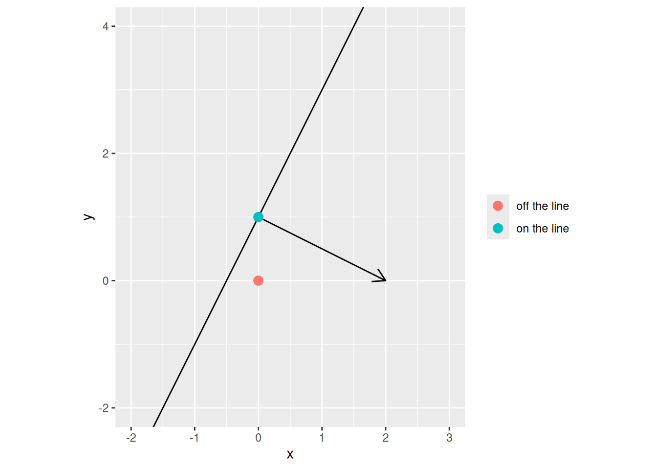

A straight line rising to the right through the point (0, 1). An arrow from (0, 1) points right and down, perpendicular to the line. A second point at the origin lies below the line. — Figure 1: The graph of $y = 2x + 1$, a line in the plane, with its normal vector $(2, -1)$ drawn from the point $(0, 1)$ on it and the point $(0, 0)$ off it

Exercise 26 (Finding the normal vector of the graph of a regression surface) Theorem 15 says that the graph of $\mathord{\smash[b]{\underset{\raise.3ex\hbox{$\scriptstyle\sim$}}{x}}\vphantom{x}}\mapsto \mathord{\smash[b]{\underset{\raise.3ex\hbox{$\scriptstyle\sim$}}{w}}\vphantom{w}} \cdot \mathord{\smash[b]{\underset{\raise.3ex\hbox{$\scriptstyle\sim$}}{x}}\vphantom{x}} + b$ is a hyperplane in $\mathbb{R}^{p+1}$. Let $f(x_1, x_2) = 3 x_1 - x_2 + 2$, a regression surface with two features.

Find a normal vector for the graph of $f$ in $\mathbb{R}^3$.

Hint

Read off $\mathord{\smash[b]{\underset{\raise.3ex\hbox{$\scriptstyle\sim$}}{w}}\vphantom{w}}$ and use the normal vector $\begin{bmatrix}\mathord{\smash[b]{\underset{\raise.3ex\hbox{$\scriptstyle\sim$}}{w}}\vphantom{w}}\\ -1\end{bmatrix}$ from Theorem 15.

Solution 26. Here $\mathord{\smash[b]{\underset{\raise.3ex\hbox{$\scriptstyle\sim$}}{w}}\vphantom{w}}= (3, -1)$ and $b = 2$. By Theorem 15, the graph of $f$ is a hyperplane in $\mathbb{R}^3$ with normal vector $(3, -1, -1)$: it holds the points $(x_1, x_2, y)$ with $3 x_1 - x_2 - y + 2 = 0$.

Definition 9 (Open half-space) Let $\mathcal{H} = \mathopen{}\left\{\mathord{\smash[b]{\underset{\raise.3ex\hbox{$\scriptstyle\sim$}}{x}}\vphantom{x}}\in \mathbb{R}^p : \mathord{\smash[b]{\underset{\raise.3ex\hbox{$\scriptstyle\sim$}}{w}}\vphantom{w}} \cdot \mathord{\smash[b]{\underset{\raise.3ex\hbox{$\scriptstyle\sim$}}{x}}\vphantom{x}} + b = 0\right\}\mathclose{}$ be a hyperplane (Definition 27 in Matrices). The two open half-spaces [7] of $\mathcal{H}$ are

\[ \mathcal{H}^+ \stackrel{\text{def}}{=}\mathopen{}\left\{\mathord{\smash[b]{\underset{\raise.3ex\hbox{$\scriptstyle\sim$}}{x}}\vphantom{x}}\in \mathbb{R}^p : \mathord{\smash[b]{\underset{\raise.3ex\hbox{$\scriptstyle\sim$}}{w}}\vphantom{w}} \cdot \mathord{\smash[b]{\underset{\raise.3ex\hbox{$\scriptstyle\sim$}}{x}}\vphantom{x}} + b > 0\right\}\mathclose{} \quad \text{and} \quad \mathcal{H}^- \stackrel{\text{def}}{=}\mathopen{}\left\{\mathord{\smash[b]{\underset{\raise.3ex\hbox{$\scriptstyle\sim$}}{x}}\vphantom{x}}\in \mathbb{R}^p : \mathord{\smash[b]{\underset{\raise.3ex\hbox{$\scriptstyle\sim$}}{w}}\vphantom{w}} \cdot \mathord{\smash[b]{\underset{\raise.3ex\hbox{$\scriptstyle\sim$}}{x}}\vphantom{x}} + b < 0\right\}\mathclose{}. \tag{1}\]

Definition 10 (Closed half-space) The closed half-spaces of the hyperplane $\mathcal{H}$ of Definition 9 also include $\mathcal{H}$ itself: $\mathcal{H}^+ \cup \mathcal{H}$ and $\mathcal{H}^- \cup \mathcal{H}$.

Example 25 (Half-spaces of a line in the plane) Let $\mathcal{H}$ be the line in $\mathbb{R}^2$ with $\mathord{\smash[b]{\underset{\raise.3ex\hbox{$\scriptstyle\sim$}}{w}}\vphantom{w}} = (1, 2)$ and $b = -2$ (Definition 27 in Matrices), so $\mathcal{H} = \mathopen{}\left\{\mathord{\smash[b]{\underset{\raise.3ex\hbox{$\scriptstyle\sim$}}{x}}\vphantom{x}}: x_1 + 2 x_2 - 2 = 0\right\}\mathclose{}$. Evaluate $\mathord{\smash[b]{\underset{\raise.3ex\hbox{$\scriptstyle\sim$}}{w}}\vphantom{w}} \cdot \mathord{\smash[b]{\underset{\raise.3ex\hbox{$\scriptstyle\sim$}}{x}}\vphantom{x}} + b$ at three points (Definition 9):

At $(0, 0)$ it equals $0 + 0 - 2 = -2 < 0$, so $(0, 0) \in \mathcal{H}^-$.
At $(2, 0)$ it equals $2 + 0 - 2 = 0$, so $(2, 0) \in \mathcal{H}$.
At $(2, 1)$ it equals $2 + 2 - 2 = 2 > 0$, so $(2, 1) \in \mathcal{H}^+$.

Moving from $(2, 0)$ in the direction $\mathord{\smash[b]{\underset{\raise.3ex\hbox{$\scriptstyle\sim$}}{w}}\vphantom{w}} = (1, 2)$ gives $(3, 2)$, where the value is $3 + 4 - 2 = 5 > 0$. So the direction $\mathord{\smash[b]{\underset{\raise.3ex\hbox{$\scriptstyle\sim$}}{w}}\vphantom{w}}$ leads into $\mathcal{H}^+$.

Exercise 27 (Finding which open half-space holds a point) The sign of $\mathord{\smash[b]{\underset{\raise.3ex\hbox{$\scriptstyle\sim$}}{w}}\vphantom{w}} \cdot \mathord{\smash[b]{\underset{\raise.3ex\hbox{$\scriptstyle\sim$}}{x}}\vphantom{x}} + b$ tells which open half-space of a hyperplane a point $\mathord{\smash[b]{\underset{\raise.3ex\hbox{$\scriptstyle\sim$}}{x}}\vphantom{x}}$ lies in. Let $\mathcal{H}$ be the line in $\mathbb{R}^2$ with $\mathord{\smash[b]{\underset{\raise.3ex\hbox{$\scriptstyle\sim$}}{w}}\vphantom{w}} = (2, -1)$ and $b = -1$.

Decide whether $(0, 0)$ is in $\mathcal{H}^+$ or in $\mathcal{H}^-$.

Hint

Evaluate $\mathord{\smash[b]{\underset{\raise.3ex\hbox{$\scriptstyle\sim$}}{w}}\vphantom{w}} \cdot \mathord{\smash[b]{\underset{\raise.3ex\hbox{$\scriptstyle\sim$}}{x}}\vphantom{x}} + b$ at $(0, 0)$.

Solution 27. At $(0, 0)$, $\mathord{\smash[b]{\underset{\raise.3ex\hbox{$\scriptstyle\sim$}}{w}}\vphantom{w}} \cdot \mathord{\smash[b]{\underset{\raise.3ex\hbox{$\scriptstyle\sim$}}{x}}\vphantom{x}} + b = 0 + 0 - 1 = -1 < 0$, so $(0, 0)$ is in the open half-space $\mathcal{H}^-$.

Exercise 28 (Testing whether a point is in a closed half-space) A closed half-space adds the hyperplane itself to an open half-space. Let $\mathcal{H}$ be the line in $\mathbb{R}^2$ with $\mathord{\smash[b]{\underset{\raise.3ex\hbox{$\scriptstyle\sim$}}{w}}\vphantom{w}} = (2, -1)$ and $b = -3$.

Decide whether the point $(2, 1)$ is in the closed half-space $\mathcal{H}^+ \cup \mathcal{H}$.

Hint

Solution 28. At $(2, 1)$, $\mathord{\smash[b]{\underset{\raise.3ex\hbox{$\scriptstyle\sim$}}{w}}\vphantom{w}} \cdot \mathord{\smash[b]{\underset{\raise.3ex\hbox{$\scriptstyle\sim$}}{x}}\vphantom{x}} + b = 4 - 1 - 3 = 0$, so $(2, 1) \in \mathcal{H}$. It is therefore in the closed half-space $\mathcal{H}^+ \cup \mathcal{H}$, though not in the open half-space $\mathcal{H}^+$.

Remark 2 (The two sides of a hyperplane). Every point of $\mathbb{R}^p$ is in exactly one of $\mathcal{H}^+$, $\mathcal{H}$ and $\mathcal{H}^-$, because the number $\mathord{\smash[b]{\underset{\raise.3ex\hbox{$\scriptstyle\sim$}}{w}}\vphantom{w}} \cdot \mathord{\smash[b]{\underset{\raise.3ex\hbox{$\scriptstyle\sim$}}{x}}\vphantom{x}} + b$ is positive, zero or negative. The vector $\mathord{\smash[b]{\underset{\raise.3ex\hbox{$\scriptstyle\sim$}}{w}}\vphantom{w}}$ points into $\mathcal{H}^+$: the number $\mathord{\smash[b]{\underset{\raise.3ex\hbox{$\scriptstyle\sim$}}{w}}\vphantom{w}} \cdot \mathord{\smash[b]{\underset{\raise.3ex\hbox{$\scriptstyle\sim$}}{x}}\vphantom{x}} + b$ goes up when $\mathord{\smash[b]{\underset{\raise.3ex\hbox{$\scriptstyle\sim$}}{x}}\vphantom{x}}$ moves in the direction $\mathord{\smash[b]{\underset{\raise.3ex\hbox{$\scriptstyle\sim$}}{w}}\vphantom{w}}$.

Theorem 16 (Differences of points in a hyperplane and in a half-space) Let $\mathord{\smash[b]{\underset{\raise.3ex\hbox{$\scriptstyle\sim$}}{w}}\vphantom{w}} \in \mathbb{R}^p$ be nonzero, let $b \in \mathbb{R}$, and let $\mathcal{H}$, $\mathcal{H}^+$ be the hyperplane and open half-space of Definition 9. For a set $S \subseteq \mathbb{R}^p$, let $D(S) \stackrel{\text{def}}{=}\mathopen{}\left\{\mathord{\smash[b]{\underset{\raise.3ex\hbox{$\scriptstyle\sim$}}{y}}\vphantom{y}}- \mathord{\smash[b]{\underset{\raise.3ex\hbox{$\scriptstyle\sim$}}{x}}\vphantom{x}}: \mathord{\smash[b]{\underset{\raise.3ex\hbox{$\scriptstyle\sim$}}{x}}\vphantom{x}}, \mathord{\smash[b]{\underset{\raise.3ex\hbox{$\scriptstyle\sim$}}{y}}\vphantom{y}}\in S\right\}\mathclose{}$ be the set of differences of its points.

$D(\mathcal{H}) = \mathopen{}\left\{\mathord{\smash[b]{\underset{\raise.3ex\hbox{$\scriptstyle\sim$}}{s}}\vphantom{s}} : \mathord{\smash[b]{\underset{\raise.3ex\hbox{$\scriptstyle\sim$}}{w}}\vphantom{w}} \cdot \mathord{\smash[b]{\underset{\raise.3ex\hbox{$\scriptstyle\sim$}}{s}}\vphantom{s}} = 0\right\}\mathclose{}$, a subspace of dimension $p - 1$.
$D(\mathcal{H}^+) = \mathbb{R}^p$, a subspace of dimension $p$.

The same holds for $\mathcal{H}^-$.

Proof. Part 1. Let $\mathord{\smash[b]{\underset{\raise.3ex\hbox{$\scriptstyle\sim$}}{x}}\vphantom{x}}, \mathord{\smash[b]{\underset{\raise.3ex\hbox{$\scriptstyle\sim$}}{y}}\vphantom{y}}\in \mathcal{H}$. By Theorem 13 part 3, $\mathord{\smash[b]{\underset{\raise.3ex\hbox{$\scriptstyle\sim$}}{w}}\vphantom{w}} \cdot (\mathord{\smash[b]{\underset{\raise.3ex\hbox{$\scriptstyle\sim$}}{y}}\vphantom{y}}- \mathord{\smash[b]{\underset{\raise.3ex\hbox{$\scriptstyle\sim$}}{x}}\vphantom{x}}) = 0$, so $\mathord{\smash[b]{\underset{\raise.3ex\hbox{$\scriptstyle\sim$}}{y}}\vphantom{y}}- \mathord{\smash[b]{\underset{\raise.3ex\hbox{$\scriptstyle\sim$}}{x}}\vphantom{x}}\in \mathcal{H}_0 = \mathopen{}\left\{\mathord{\smash[b]{\underset{\raise.3ex\hbox{$\scriptstyle\sim$}}{s}}\vphantom{s}} : \mathord{\smash[b]{\underset{\raise.3ex\hbox{$\scriptstyle\sim$}}{w}}\vphantom{w}} \cdot \mathord{\smash[b]{\underset{\raise.3ex\hbox{$\scriptstyle\sim$}}{s}}\vphantom{s}} = 0\right\}\mathclose{}$. Conversely, take any $\mathord{\smash[b]{\underset{\raise.3ex\hbox{$\scriptstyle\sim$}}{x}}\vphantom{x}}_0 \in \mathcal{H}$ (Theorem 13 part 2 gives such a point). For any $\mathord{\smash[b]{\underset{\raise.3ex\hbox{$\scriptstyle\sim$}}{s}}\vphantom{s}} \in \mathcal{H}_0$, the point $\mathord{\smash[b]{\underset{\raise.3ex\hbox{$\scriptstyle\sim$}}{x}}\vphantom{x}}_0 + \mathord{\smash[b]{\underset{\raise.3ex\hbox{$\scriptstyle\sim$}}{s}}\vphantom{s}}$ is in $\mathcal{H}$ by the same part, and $(\mathord{\smash[b]{\underset{\raise.3ex\hbox{$\scriptstyle\sim$}}{x}}\vphantom{x}}_0 + \mathord{\smash[b]{\underset{\raise.3ex\hbox{$\scriptstyle\sim$}}{s}}\vphantom{s}}) - \mathord{\smash[b]{\underset{\raise.3ex\hbox{$\scriptstyle\sim$}}{x}}\vphantom{x}}_0 = \mathord{\smash[b]{\underset{\raise.3ex\hbox{$\scriptstyle\sim$}}{s}}\vphantom{s}}$. So $D(\mathcal{H}) = \mathcal{H}_0$, which has dimension $p - 1$ by Theorem 13 part 1.

Part 2. Every difference is in $\mathbb{R}^p$, so $D(\mathcal{H}^+) \subseteq \mathbb{R}^p$. For the reverse inclusion, take any $\mathord{\smash[b]{\underset{\raise.3ex\hbox{$\scriptstyle\sim$}}{x}}\vphantom{x}}_0 \in \mathcal{H}$. Take any $\mathord{\smash[b]{\underset{\raise.3ex\hbox{$\scriptstyle\sim$}}{v}}\vphantom{v}} \in \mathbb{R}^p$. For a number $t > 0$ to be chosen, let $\mathord{\smash[b]{\underset{\raise.3ex\hbox{$\scriptstyle\sim$}}{x}}\vphantom{x}}_t \stackrel{\text{def}}{=}\mathord{\smash[b]{\underset{\raise.3ex\hbox{$\scriptstyle\sim$}}{x}}\vphantom{x}}_0 + t\,\mathord{\smash[b]{\underset{\raise.3ex\hbox{$\scriptstyle\sim$}}{w}}\vphantom{w}}$. Then

\[ \begin{aligned} \mathord{\smash[b]{\underset{\raise.3ex\hbox{$\scriptstyle\sim$}}{w}}\vphantom{w}} \cdot \mathord{\smash[b]{\underset{\raise.3ex\hbox{$\scriptstyle\sim$}}{x}}\vphantom{x}}_t + b &= \mathopen{}\left(\mathord{\smash[b]{\underset{\raise.3ex\hbox{$\scriptstyle\sim$}}{w}}\vphantom{w}} \cdot \mathord{\smash[b]{\underset{\raise.3ex\hbox{$\scriptstyle\sim$}}{x}}\vphantom{x}}_0 + b\right)\mathclose{} + t\,\mathord{\smash[b]{\underset{\raise.3ex\hbox{$\scriptstyle\sim$}}{w}}\vphantom{w}} \cdot \mathord{\smash[b]{\underset{\raise.3ex\hbox{$\scriptstyle\sim$}}{w}}\vphantom{w}} && \text{(linearity of } \mathord{\smash[b]{\underset{\raise.3ex\hbox{$\scriptstyle\sim$}}{x}}\vphantom{x}}\mapsto \mathord{\smash[b]{\underset{\raise.3ex\hbox{$\scriptstyle\sim$}}{w}}\vphantom{w}} \cdot \mathord{\smash[b]{\underset{\raise.3ex\hbox{$\scriptstyle\sim$}}{x}}\vphantom{x}} \text{)} \\ &= t\,\mathord{\smash[b]{\underset{\raise.3ex\hbox{$\scriptstyle\sim$}}{w}}\vphantom{w}} \cdot \mathord{\smash[b]{\underset{\raise.3ex\hbox{$\scriptstyle\sim$}}{w}}\vphantom{w}}, && \text{(} \mathord{\smash[b]{\underset{\raise.3ex\hbox{$\scriptstyle\sim$}}{x}}\vphantom{x}}_0 \in \mathcal{H} \text{)} \end{aligned} \]

which is positive, so $\mathord{\smash[b]{\underset{\raise.3ex\hbox{$\scriptstyle\sim$}}{x}}\vphantom{x}}_t \in \mathcal{H}^+$. Next,

\[ \begin{aligned} \mathord{\smash[b]{\underset{\raise.3ex\hbox{$\scriptstyle\sim$}}{w}}\vphantom{w}} \cdot (\mathord{\smash[b]{\underset{\raise.3ex\hbox{$\scriptstyle\sim$}}{x}}\vphantom{x}}_t + \mathord{\smash[b]{\underset{\raise.3ex\hbox{$\scriptstyle\sim$}}{v}}\vphantom{v}}) + b &= \mathopen{}\left(\mathord{\smash[b]{\underset{\raise.3ex\hbox{$\scriptstyle\sim$}}{w}}\vphantom{w}} \cdot \mathord{\smash[b]{\underset{\raise.3ex\hbox{$\scriptstyle\sim$}}{x}}\vphantom{x}}_t + b\right)\mathclose{} + \mathord{\smash[b]{\underset{\raise.3ex\hbox{$\scriptstyle\sim$}}{w}}\vphantom{w}} \cdot \mathord{\smash[b]{\underset{\raise.3ex\hbox{$\scriptstyle\sim$}}{v}}\vphantom{v}} && \text{(linearity of } \mathord{\smash[b]{\underset{\raise.3ex\hbox{$\scriptstyle\sim$}}{x}}\vphantom{x}}\mapsto \mathord{\smash[b]{\underset{\raise.3ex\hbox{$\scriptstyle\sim$}}{w}}\vphantom{w}} \cdot \mathord{\smash[b]{\underset{\raise.3ex\hbox{$\scriptstyle\sim$}}{x}}\vphantom{x}} \text{)} \\ &= t\,\mathord{\smash[b]{\underset{\raise.3ex\hbox{$\scriptstyle\sim$}}{w}}\vphantom{w}} \cdot \mathord{\smash[b]{\underset{\raise.3ex\hbox{$\scriptstyle\sim$}}{w}}\vphantom{w}} + \mathord{\smash[b]{\underset{\raise.3ex\hbox{$\scriptstyle\sim$}}{w}}\vphantom{w}} \cdot \mathord{\smash[b]{\underset{\raise.3ex\hbox{$\scriptstyle\sim$}}{v}}\vphantom{v}}. && \text{(the display above)} \end{aligned} \]

Because $\mathord{\smash[b]{\underset{\raise.3ex\hbox{$\scriptstyle\sim$}}{w}}\vphantom{w}} \cdot \mathord{\smash[b]{\underset{\raise.3ex\hbox{$\scriptstyle\sim$}}{w}}\vphantom{w}} > 0$, this is positive once $t > -\mathord{\smash[b]{\underset{\raise.3ex\hbox{$\scriptstyle\sim$}}{w}}\vphantom{w}} \cdot \mathord{\smash[b]{\underset{\raise.3ex\hbox{$\scriptstyle\sim$}}{v}}\vphantom{v}} / \mathord{\smash[b]{\underset{\raise.3ex\hbox{$\scriptstyle\sim$}}{w}}\vphantom{w}} \cdot \mathord{\smash[b]{\underset{\raise.3ex\hbox{$\scriptstyle\sim$}}{w}}\vphantom{w}}$. Choose such a $t > 0$. Then $\mathord{\smash[b]{\underset{\raise.3ex\hbox{$\scriptstyle\sim$}}{x}}\vphantom{x}}_t$ and $\mathord{\smash[b]{\underset{\raise.3ex\hbox{$\scriptstyle\sim$}}{x}}\vphantom{x}}_t + \mathord{\smash[b]{\underset{\raise.3ex\hbox{$\scriptstyle\sim$}}{v}}\vphantom{v}}$ are both in $\mathcal{H}^+$, and their difference is $\mathord{\smash[b]{\underset{\raise.3ex\hbox{$\scriptstyle\sim$}}{v}}\vphantom{v}}$. So $\mathord{\smash[b]{\underset{\raise.3ex\hbox{$\scriptstyle\sim$}}{v}}\vphantom{v}} \in D(\mathcal{H}^+)$. The whole space $\mathbb{R}^p$ is a subspace of dimension $p$ (Definition 9 in Subspaces and Rank).

The proof for $\mathcal{H}^-$ is the same with $-\mathord{\smash[b]{\underset{\raise.3ex\hbox{$\scriptstyle\sim$}}{w}}\vphantom{w}}$ and $-b$ in place of $\mathord{\smash[b]{\underset{\raise.3ex\hbox{$\scriptstyle\sim$}}{w}}\vphantom{w}}$ and $b$.

Example 26 (Two iris species on either side of a line) The iris data set in R has the petal length and petal width, in centimeters, of 150 irises. Take the 100 flowers of the species versicolor and virginica, and let $\mathord{\smash[b]{\underset{\raise.3ex\hbox{$\scriptstyle\sim$}}{x}}\vphantom{x}}= (x_1, x_2)$ be the petal length and petal width of one flower. A logistic regression of the species on $\mathord{\smash[b]{\underset{\raise.3ex\hbox{$\scriptstyle\sim$}}{x}}\vphantom{x}}$ gives a coefficient vector $\mathord{\smash[b]{\underset{\raise.3ex\hbox{$\scriptstyle\sim$}}{w}}\vphantom{w}}$ and an intercept $b$. The line $\mathord{\smash[b]{\underset{\raise.3ex\hbox{$\scriptstyle\sim$}}{w}}\vphantom{w}} \cdot \mathord{\smash[b]{\underset{\raise.3ex\hbox{$\scriptstyle\sim$}}{x}}\vphantom{x}} + b = 0$ is a hyperplane in $\mathbb{R}^2$ (Definition 27 in Matrices), and the two species mostly fall in its two open half-spaces (Definition 9). Figure 2 shows the line and the flowers.

[Code]

two_species <- dplyr::filter(iris, Species != "setosa") |> droplevels()
fit <- glm(
  Species ~ Petal.Length + Petal.Width,
  family = binomial,
  data = two_species
)
w <- coef(fit)[c("Petal.Length", "Petal.Width")]
b <- coef(fit)[["(Intercept)"]]
two_species$score <- as.vector(
  as.matrix(two_species[c("Petal.Length", "Petal.Width")]) %*% w + b
)
two_species$side <- ifelse(two_species$score > 0, "positive", "negative")
ggplot2::ggplot(two_species) +
  ggplot2::aes(x = Petal.Length, y = Petal.Width, colour = Species) +
  ggplot2::geom_point() +
  ggplot2::geom_abline(intercept = -b / w[[2]], slope = -w[[1]] / w[[2]]) +
  ggplot2::labs(x = "Petal length (cm)", y = "Petal width (cm)")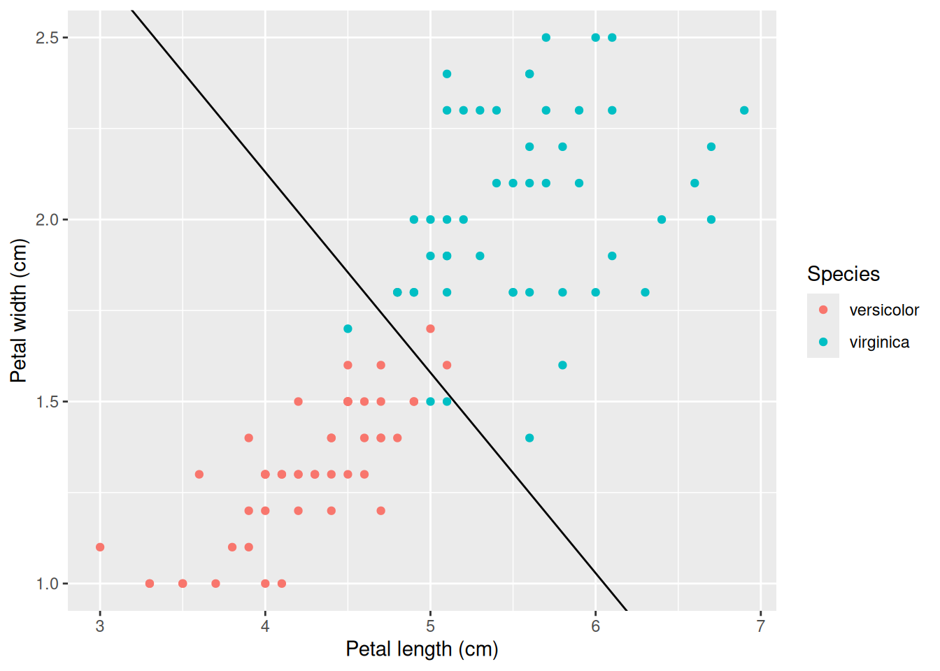

Scatter plot of petal width against petal length for 100 irises. Versicolor points, in one color, are mostly to the lower left. Virginica points, in another color, are mostly to the upper right. A straight line runs between the two groups and separates most of them. — Figure 2: Petal length and width of versicolor and virginica irises, with the line where a logistic regression is indifferent between the two species

table(two_species$Species, two_species$side)
#>             
#>              negative positive
#>   versicolor       47        3
#>   virginica         3       47

The vector $\mathord{\smash[b]{\underset{\raise.3ex\hbox{$\scriptstyle\sim$}}{w}}\vphantom{w}}$ points toward the virginica side, so the positive half-space $\mathcal{H}^+$ holds 50 of the 100 flowers, and 47 of them are virginica. The line is a set of dimension $p - 1 = 1$, and each side is a region of the plane of dimension $p = 2$ (Theorem 16).

Exercise 29 (Which side of the plane?) Let $\mathcal{H}$ be the plane in $\mathbb{R}^3$ with $\mathord{\smash[b]{\underset{\raise.3ex\hbox{$\scriptstyle\sim$}}{w}}\vphantom{w}} = (1, 1, 1)$ and $b = -1$ (Example 22).

For each point, say whether it is in $\mathcal{H}^+$, $\mathcal{H}$ or $\mathcal{H}^-$ (Definition 9): $(0, 0, 0)$, $(1, 0, 0)$ and $(1, 1, 1)$.
Write the plane and its half-spaces using $-\mathord{\smash[b]{\underset{\raise.3ex\hbox{$\scriptstyle\sim$}}{w}}\vphantom{w}}$ and $-b$. Which points from part 1 change sides?
State the dimension of $D(\mathcal{H})$ and of $D(\mathcal{H}^+)$ (Theorem 16).

Solution 29.

Compute $\mathord{\smash[b]{\underset{\raise.3ex\hbox{$\scriptstyle\sim$}}{w}}\vphantom{w}} \cdot \mathord{\smash[b]{\underset{\raise.3ex\hbox{$\scriptstyle\sim$}}{x}}\vphantom{x}} + b = x_1 + x_2 + x_3 - 1$ at each point.
- At $(0, 0, 0)$ it equals $0 + 0 + 0 - 1 = -1 < 0$, so the point is in $\mathcal{H}^-$.
- At $(1, 0, 0)$ it equals $1 + 0 + 0 - 1 = 0$, so the point is in $\mathcal{H}$.
- At $(1, 1, 1)$ it equals $1 + 1 + 1 - 1 = 2 > 0$, so the point is in $\mathcal{H}^+$.
With $-\mathord{\smash[b]{\underset{\raise.3ex\hbox{$\scriptstyle\sim$}}{w}}\vphantom{w}} = (-1, -1, -1)$ and $-b = 1$, the equation is $-x_1 - x_2 - x_3 + 1 = 0$. Multiplying both sides by $-1$ gives the original equation, so it is the same plane. The new expression is the negative of the old one at every point, so the new positive half-space is the old $\mathcal{H}^-$ and the new negative half-space is the old $\mathcal{H}^+$. The origin $(0, 0, 0)$ is now in the positive half-space, and $(1, 1, 1)$ is now in the negative half-space. The point $(1, 0, 0)$ stays on the plane. So the origin and $(1, 1, 1)$ both change names, and the point on the plane does not.
Here $p = 3$. $D(\mathcal{H})$ is the subspace $\mathopen{}\left\{\mathord{\smash[b]{\underset{\raise.3ex\hbox{$\scriptstyle\sim$}}{s}}\vphantom{s}} : s_1 + s_2 + s_3 = 0\right\}\mathclose{}$, which has dimension $p - 1 = 2$. $D(\mathcal{H}^+) = \mathbb{R}^3$ has dimension $p = 3$.

Definition 11 (Rank factorization) Let $\mathbf{A}$ be an $m \times n$ matrix with $\operatorname{rank}(\mathbf{A}) = r \ge 1$. A rank factorization [8] of $\mathbf{A}$ is a product

\[ \underbrace{\mathbf{A}}_{m \times n} = \underbrace{\mathbf{C}}_{m \times r}\,\underbrace{\mathbf{R}}_{r \times n}. \]

Example 27 (A rank factorization of a rank-one matrix) The matrix $\mathbf{A}$ in Example 1 has rank $1$ (Example 11), and

\[ \begin{aligned} \begin{bmatrix} 1 \\ 3 \end{bmatrix} \begin{bmatrix} 1 & -2 & -2 \end{bmatrix} &= \begin{bmatrix} 1 \cdot 1 & 1 \cdot(-2) & 1 \cdot(-2) \\ 3 \cdot 1 & 3 \cdot(-2) & 3 \cdot(-2) \end{bmatrix} \\ &= \begin{bmatrix} 1 & -2 & -2 \\ 3 & -6 & -6 \end{bmatrix}, \end{aligned} \]

so $\mathbf{C} = \begin{bmatrix} 1 \\ 3 \end{bmatrix}$ ($2 \times 1$) and $\mathbf{R} = \begin{bmatrix} 1 & -2 & -2 \end{bmatrix}$ ($1 \times 3$) are a rank factorization. It is not unique: $\mathbf{C} = \begin{bmatrix} 2 \\ 6 \end{bmatrix}$ and $\mathbf{R} = \begin{bmatrix} \frac{1}{2} & -1 & -1 \end{bmatrix}$ give the same product. A product $\mathbf{C} \mathbf{R}$ with $\mathbf{C}$ of size $2 \times 2$ is not a rank factorization of this $\mathbf{A}$, because the inner dimension must equal $\operatorname{rank}(\mathbf{A}) = 1$.

Theorem 17 (Every nonzero matrix has a rank factorization) Every $m \times n$ matrix $\mathbf{A}$ with $\operatorname{rank}(\mathbf{A}) = r \ge 1$ has a rank factorization (Definition 11). One is given by taking the columns of $\mathbf{C}$ to be any basis of $\mathcal{C}(\mathbf{A})$.

Proof. $\mathcal{C}(\mathbf{A})$ has dimension $r$ (Theorem 7), so it has a basis $\mathord{\smash[b]{\underset{\raise.3ex\hbox{$\scriptstyle\sim$}}{c}}\vphantom{c}}_1, \ldots, \mathord{\smash[b]{\underset{\raise.3ex\hbox{$\scriptstyle\sim$}}{c}}\vphantom{c}}_r$ (Theorem 9 in Subspaces and Rank); let $\mathbf{C}$ be the $m \times r$ matrix with these columns. Each column $\mathord{\smash[b]{\underset{\raise.3ex\hbox{$\scriptstyle\sim$}}{a}}\vphantom{a}}_j$ of $\mathbf{A}$ is in $\mathcal{C}(\mathbf{A})$, so $\mathord{\smash[b]{\underset{\raise.3ex\hbox{$\scriptstyle\sim$}}{a}}\vphantom{a}}_j = r_{1j} \mathord{\smash[b]{\underset{\raise.3ex\hbox{$\scriptstyle\sim$}}{c}}\vphantom{c}}_1 + \cdots + r_{rj} \mathord{\smash[b]{\underset{\raise.3ex\hbox{$\scriptstyle\sim$}}{c}}\vphantom{c}}_r$ for some numbers $r_{ij}$, because the basis spans $\mathcal{C}(\mathbf{A})$. Let $\mathbf{R}$ be the $r \times n$ matrix with entries $r_{ij}$, whose column $j$ is $\mathord{\smash[b]{\underset{\raise.3ex\hbox{$\scriptstyle\sim$}}{r}}\vphantom{r}}_j = (r_{1j}, \ldots, r_{rj})$. Then column $j$ of $\mathbf{C} \mathbf{R}$ is

\[ \begin{aligned} \mathbf{C} \mathord{\smash[b]{\underset{\raise.3ex\hbox{$\scriptstyle\sim$}}{r}}\vphantom{r}}_j &= r_{1j} \mathord{\smash[b]{\underset{\raise.3ex\hbox{$\scriptstyle\sim$}}{c}}\vphantom{c}}_1 + \cdots + r_{rj} \mathord{\smash[b]{\underset{\raise.3ex\hbox{$\scriptstyle\sim$}}{c}}\vphantom{c}}_r && \text{(}\href{linear-algebra-subspaces.qmd#thm-matvec-columns}{\text{Theorem~3 in Subspaces and Rank}}\text{)} \\ &= \mathord{\smash[b]{\underset{\raise.3ex\hbox{$\scriptstyle\sim$}}{a}}\vphantom{a}}_j, && \text{(choice of the } r_{ij} \text{)} \end{aligned} \]

so $\mathbf{C} \mathbf{R} = \mathbf{A}$.

Example 28 (Building a rank factorization from a basis) For $\mathbf{A}$ in Example 1, $(1, 3)$ spans $\mathcal{C}(\mathbf{A})$ (Example 2), and it is linearly independent because it is nonzero ($c\,(1, 3) = \mathord{\smash[b]{\underset{\raise.3ex\hbox{$\scriptstyle\sim$}}{0}}\vphantom{0}}_2$ forces $c = 0$), so it is a basis of $\mathcal{C}(\mathbf{A})$. The columns of $\mathbf{A}$ are $(1, 3) = 1 \cdot(1, 3)$, $(-2, -6) = -2 \cdot(1, 3)$ and $(-2, -6) = -2 \cdot(1, 3)$, so the construction in Theorem 17 gives $\mathbf{C} = \begin{bmatrix} 1 \\ 3 \end{bmatrix}$ and $\mathbf{R} = \begin{bmatrix} 1 & -2 & -2 \end{bmatrix}$, the factorization in Example 27.

Exercise 30 (Finding a rank factorization of a rank-one matrix) A rank factorization writes an $m \times n$ matrix with rank $r$ as a matrix product of an $m \times r$ and an $r \times n$ matrix. Let

\[ \mathbf{A} = \begin{bmatrix}2 & 4 \\ 1 & 2\end{bmatrix}. \]

Find a rank factorization of $\mathbf{A}$.

Hint

In $\mathbf{A}$, the second column is twice the first, so ${\operatorname{rank}\mathopen{}\left(\mathbf{A}\right)\mathclose{}} = 1$.

Solution 30. Columns of $\mathbf{A}$ are $(2, 1)$ and $(4, 2) = 2\,(2, 1)$, so ${\operatorname{rank}\mathopen{}\left(\mathbf{A}\right)\mathclose{}} = 1$, and

\[ \begin{bmatrix}2 \\ 1\end{bmatrix} \begin{bmatrix}1 & 2\end{bmatrix} = \begin{bmatrix}2 \cdot 1 & 2 \cdot 2 \\ 1 \cdot 1 & 1 \cdot 2\end{bmatrix} = \begin{bmatrix}2 & 4 \\ 1 & 2\end{bmatrix} = \mathbf{A}. \]

So $\mathbf{C} = \begin{bmatrix}2 \\ 1\end{bmatrix}$ ($2 \times 1$) and $\mathbf{R} = \begin{bmatrix}1 & 2\end{bmatrix}$ ($1 \times 2$) are a rank factorization.

Exercise 31 (Building a rank factorization from a basis of the column space) Theorem 17 builds a rank factorization from a basis of the column space. Let

\[ \mathbf{A} = \begin{bmatrix}1 & 2 & 3 \\ 2 & 4 & 6 \\ 1 & 0 & 1\end{bmatrix}, \]

in which column $3$ is column $1$ plus column $2$.

Find a rank factorization $\mathbf{A} = \mathbf{C}\mathbf{R}$ in which $\mathbf{C}$ holds columns 1 and 2 of $\mathbf{A}$.

Hint

Column $j$ of $\mathbf{R}$ says how much of column $1$ and of column $2$ of $\mathbf{C}$ add up to column $j$ of $\mathbf{A}$.

Solution 31. Columns 1 and 2 of $\mathbf{A}$, $(1, 2, 1)$ and $(2, 4, 0)$, are linearly independent: the third entry of $c_1\,(1, 2, 1) + c_2\,(2, 4, 0)$ is $c_1$, and then the first is $2 c_2$. They span $\mathcal{C}(\mathbf{A})$, since the third column is the first plus the second, so ${\operatorname{rank}\mathopen{}\left(\mathbf{A}\right)\mathclose{}} = 2$. Each column of $\mathbf{A}$ in terms of them:

\[ \begin{aligned} (1, 2, 1) &= 1 \cdot(1, 2, 1) + 0 \cdot(2, 4, 0), \\ (2, 4, 0) &= 0 \cdot(1, 2, 1) + 1 \cdot(2, 4, 0), \\ (3, 6, 1) &= 1 \cdot(1, 2, 1) + 1 \cdot(2, 4, 0). \end{aligned} \]

\[ \mathbf{C} = \begin{bmatrix}1 & 2 \\ 2 & 4 \\ 1 & 0\end{bmatrix}, \qquad \mathbf{R} = \begin{bmatrix}1 & 0 & 1 \\ 0 & 1 & 1\end{bmatrix}, \]

and multiplying gives back $\mathbf{A}$.

[1]

Wikipedia contributors, “Row and column spaces — Wikipedia, the free encyclopedia.” 2026. Available: https://en.wikipedia.org/wiki/Row_and_column_spaces

[2]

“Chapter I: Linear algebra, basic notions.” Lecture notes, Department of Mathematics, Northwestern University. Available: https://sites.math.northwestern.edu/len/LinAlg/chap1.pdf

[3]

Wikipedia contributors, “Gram matrix — Wikipedia, the free encyclopedia.” 2026. Available: https://en.wikipedia.org/wiki/Gram_matrix

[4]

H. Zhou, “Rank and nullity.” Lecture notes for Biostat 216, Mathematical Methods for Biostatistics, University of California, Los Angeles, 2024. Accessed: Oct. 05, 2026. [Online]. Available: https://ucla-biostat-216.github.io/2024fall/slides/05-rank/05-rank.html

[5]

Wikipedia contributors, “Rank–nullity theorem — Wikipedia, the free encyclopedia.” 2026. Available: https://en.wikipedia.org/wiki/Rank%E2%80%93nullity_theorem

[6]

Wikipedia contributors, “Affine space — Wikipedia, the free encyclopedia.” 2026. Available: https://en.wikipedia.org/wiki/Affine_space

[7]

Wikipedia contributors, “Half-space (geometry) — Wikipedia, the free encyclopedia.” 2026. Available: https://en.wikipedia.org/wiki/Half-space_(geometry)

[8]

Wikipedia contributors, “Rank factorization — Wikipedia, the free encyclopedia.” 2026. Available: https://en.wikipedia.org/wiki/Rank_factorization