Quadratic Minimization under Linear Constraints

Last modified: 2026-11-03 15:17:03 (PST)

Source

This section is adapted from the Lagrange-multiplier part of Zhou [1], used under the MIT License (see the license text in Linear Algebra). The source solves the stationarity equations of the Lagrangian and reports the solution; here the solution is also proved to be the unique minimizer, directly from the positive definiteness of the matrices involved. The source assumes only that \(\mathbf{S}\) is positive definite; the added hypothesis that the columns of \(\mathbf{A}\) are linearly independent makes \({\mathbf{A}}^{\top} \mathbf{S}^{-1} \mathbf{A}\) invertible. The source’s example with general coefficients \(a_1, a_2, b\) is specialized here to \(3, 4, 5\). These parts of the source are not part of this section:

• the Lagrange multiplier method for constraints that are not linear, or objectives that are not quadratic, including its multinomial maximum likelihood example
• the eigenvalues of the block matrix of the stationarity equations, and the convexity of the Lagrangian in \(\mathord{\smash[b]{\underset{\raise.3ex\hbox{$\scriptstyle\sim$}}{x}}\vphantom{x}}\) and its concavity in the multipliers
• its homework examples

Definition 1 (Feasible set) In a problem that looks for a best point among some allowed points of \(\mathbb{R}^p\), the set \(F \subseteq \mathbb{R}^p\) of allowed points is the feasible set, [2] and its points are feasible.

Definition 2 (Constraints) When the feasible set \(F\) (Definition 1) is the set of points that satisfy some equations or inequalities, those equations or inequalities are the constraints.

Example 1 (A line as a feasible set) With the single constraint \(3 x_1 + 4 x_2 = 5\), the feasible set is the line \(\mathopen{}\left\{\mathord{\smash[b]{\underset{\raise.3ex\hbox{$\scriptstyle\sim$}}{x}}\vphantom{x}}\in \mathbb{R}^2 : 3 x_1 + 4 x_2 = 5\right\}\mathclose{}\). \({(1, 0.5)}^{\top}\) is feasible, since

\[ \begin{aligned} 3 \cdot 1 + 4 \cdot 0.5 &= 3 + 2 \\ &= 5; \end{aligned} \]

\(\mathord{\smash[b]{\underset{\raise.3ex\hbox{$\scriptstyle\sim$}}{0}}\vphantom{0}}\) is not feasible, since \(3 \cdot 0 + 4 \cdot 0 = 0 \ne 5\).

Definition 3 (Objective function, objective) Let \(f : \mathbb{R}^p \to \mathbb{R}\) and let \(F \subseteq \mathbb{R}^p\) be a feasible set (Definition 1). In the problem of minimizing \(f\) over \(F\), \(f\) is the objective function (or objective).

Definition 4 (Minimizer over a feasible set) With \(f\) and \(F\) as in Definition 3, a minimizer of \(f\) over \(F\) is a feasible \(\mathord{\smash[b]{\underset{\raise.3ex\hbox{$\scriptstyle\sim$}}{x}}\vphantom{x}}^*\) with \(f(\mathord{\smash[b]{\underset{\raise.3ex\hbox{$\scriptstyle\sim$}}{x}}\vphantom{x}}^*) \le f(\mathord{\smash[b]{\underset{\raise.3ex\hbox{$\scriptstyle\sim$}}{x}}\vphantom{x}})\) for every feasible \(\mathord{\smash[b]{\underset{\raise.3ex\hbox{$\scriptstyle\sim$}}{x}}\vphantom{x}}\): a global minimizer of \(f\) with its domain restricted to \(F\).

Definition 5 (Minimization problem) With \(f\) and \(F\) as in Definition 3, the minimization problem [3] is to find a minimizer of \(f\) over \(F\) (Definition 4). When \(F\) is given by constraints (Definition 2), the problem is to minimize \(f\) subject to them.

Example 2 (Minimizing over a line) In the problem of minimizing \(x_1^2 + x_2^2\) subject to \(3 x_1 + 4 x_2 = 5\), the objective function is \(f(\mathord{\smash[b]{\underset{\raise.3ex\hbox{$\scriptstyle\sim$}}{x}}\vphantom{x}}) = x_1^2 + x_2^2\), and the feasible set is the line of Example 1. The feasible point \({(1, 0.5)}^{\top}\) has

\[ \begin{aligned} f(1, 0.5) &= 1 + 0.25 \\ &= 1.25. \end{aligned} \]

\(\mathord{\smash[b]{\underset{\raise.3ex\hbox{$\scriptstyle\sim$}}{0}}\vphantom{0}}\) minimizes \(f\) over all of \(\mathbb{R}^2\), with \(f(\mathord{\smash[b]{\underset{\raise.3ex\hbox{$\scriptstyle\sim$}}{0}}\vphantom{0}}) = 0\), but it is not a minimizer over the feasible set, because it is not feasible.

Definition 6 (Optimization algorithm) Let:

• \(f : \mathbb{R}^p \to \mathbb{R}\): an objective function;
• \(F \subseteq \mathbb{R}^p\): a feasible set.

An optimization algorithm [3] is a step-by-step procedure that maps the pair \((f, F)\) to a feasible point \(\mathord{\smash[b]{\underset{\raise.3ex\hbox{$\scriptstyle\sim$}}{x}}\vphantom{x}}^\dagger\):

\[ (f, F) \mapsto \mathord{\smash[b]{\underset{\raise.3ex\hbox{$\scriptstyle\sim$}}{x}}\vphantom{x}}^\dagger \in F. \tag{1}\]

In words: given \((f, F)\), the procedure returns a feasible point \(\mathord{\smash[b]{\underset{\raise.3ex\hbox{$\scriptstyle\sim$}}{x}}\vphantom{x}}^\dagger\) intended to make \(f(\mathord{\smash[b]{\underset{\raise.3ex\hbox{$\scriptstyle\sim$}}{x}}\vphantom{x}}^\dagger)\) small.

Example 3 (Exhaustive search over a finite feasible set) Let \(f(\mathord{\smash[b]{\underset{\raise.3ex\hbox{$\scriptstyle\sim$}}{x}}\vphantom{x}}) = x_1^2 + x_2^2\), with the feasible set the three points \(\mathopen{}\left\{{(1, 0.5)}^{\top}, {(3, -1)}^{\top}, {(-1, 2)}^{\top}\right\}\mathclose{}\) of the line of Example 1. The procedure “evaluate \(f\) at every feasible point; return the point with the smallest value” is an optimization algorithm. Computing \(f\) at each point gives

\[ \begin{aligned} f(1, 0.5) &= 1 + 0.25 = 1.25, \\ f(3, -1) &= 9 + 1 = 10, \\ f(-1, 2) &= 1 + 4 = 5, \end{aligned} \]

so it returns \({(1, 0.5)}^{\top}\), a minimizer of \(f\) over this feasible set.

Here the objective (Definition 3) is a quadratic \(\tfrac{1}{2}\,{\mathord{\smash[b]{\underset{\raise.3ex\hbox{$\scriptstyle\sim$}}{x}}\vphantom{x}}}^{\top} \mathbf{S} \mathord{\smash[b]{\underset{\raise.3ex\hbox{$\scriptstyle\sim$}}{x}}\vphantom{x}}\) with \(\mathbf{S}\) positive definite, and the constraints (Definition 2) are \(m\) linear equations \({\mathbf{A}}^{\top} \mathord{\smash[b]{\underset{\raise.3ex\hbox{$\scriptstyle\sim$}}{x}}\vphantom{x}}= \mathord{\smash[b]{\underset{\raise.3ex\hbox{$\scriptstyle\sim$}}{b}}\vphantom{b}}\), where \(\mathbf{A}\) is a \(p \times m\) matrix and \(\mathord{\smash[b]{\underset{\raise.3ex\hbox{$\scriptstyle\sim$}}{b}}\vphantom{b}} \in \mathbb{R}^m\). The only stationary point of the objective alone (Definition 4 in Critical Points and Optimality Conditions) is \(\mathord{\smash[b]{\underset{\raise.3ex\hbox{$\scriptstyle\sim$}}{0}}\vphantom{0}}_{p \times 1}\) (its gradient is \(\mathbf{S} \mathord{\smash[b]{\underset{\raise.3ex\hbox{$\scriptstyle\sim$}}{x}}\vphantom{x}}\), and \(\mathbf{S}\) is invertible), which may not satisfy the constraints. A Lagrange multiplier adds one unknown per constraint, and the minimizer over the feasible set (Definition 1) is then found among the stationary points of a new function of the extended set of unknowns.

Definition 7 (Lagrangian) For the problem of minimizing \(f(\mathord{\smash[b]{\underset{\raise.3ex\hbox{$\scriptstyle\sim$}}{x}}\vphantom{x}})\) over \(\mathord{\smash[b]{\underset{\raise.3ex\hbox{$\scriptstyle\sim$}}{x}}\vphantom{x}}\in \mathbb{R}^p\) subject to \({\mathbf{A}}^{\top} \mathord{\smash[b]{\underset{\raise.3ex\hbox{$\scriptstyle\sim$}}{x}}\vphantom{x}}= \mathord{\smash[b]{\underset{\raise.3ex\hbox{$\scriptstyle\sim$}}{b}}\vphantom{b}}\), with \(\mathbf{A}\) a \(p \times m\) matrix and \(\mathord{\smash[b]{\underset{\raise.3ex\hbox{$\scriptstyle\sim$}}{b}}\vphantom{b}} \in \mathbb{R}^m\), the Lagrangian [4] is the function of \(\mathord{\smash[b]{\underset{\raise.3ex\hbox{$\scriptstyle\sim$}}{x}}\vphantom{x}}\in \mathbb{R}^p\) and \(\mathord{\smash[b]{\underset{\raise.3ex\hbox{$\scriptstyle\sim$}}{\lambda}}\vphantom{\lambda}}\in \mathbb{R}^m\)

\[ L(\mathord{\smash[b]{\underset{\raise.3ex\hbox{$\scriptstyle\sim$}}{x}}\vphantom{x}}, \mathord{\smash[b]{\underset{\raise.3ex\hbox{$\scriptstyle\sim$}}{\lambda}}\vphantom{\lambda}}) \stackrel{\text{def}}{=}f(\mathord{\smash[b]{\underset{\raise.3ex\hbox{$\scriptstyle\sim$}}{x}}\vphantom{x}}) + {\mathord{\smash[b]{\underset{\raise.3ex\hbox{$\scriptstyle\sim$}}{\lambda}}\vphantom{\lambda}}}^{\top} \mathopen{}\left({\mathbf{A}}^{\top} \mathord{\smash[b]{\underset{\raise.3ex\hbox{$\scriptstyle\sim$}}{x}}\vphantom{x}}- \mathord{\smash[b]{\underset{\raise.3ex\hbox{$\scriptstyle\sim$}}{b}}\vphantom{b}}\right)\mathclose{}. \]

Definition 8 (Lagrange multipliers) In the Lagrangian \(L(\mathord{\smash[b]{\underset{\raise.3ex\hbox{$\scriptstyle\sim$}}{x}}\vphantom{x}}, \mathord{\smash[b]{\underset{\raise.3ex\hbox{$\scriptstyle\sim$}}{\lambda}}\vphantom{\lambda}})\) (Definition 7), the entries of \(\mathord{\smash[b]{\underset{\raise.3ex\hbox{$\scriptstyle\sim$}}{\lambda}}\vphantom{\lambda}}\) are the Lagrange multipliers [4], one per constraint.

Example 4 (The gradients of the Lagrangian of a quadratic) Let \(f(\mathord{\smash[b]{\underset{\raise.3ex\hbox{$\scriptstyle\sim$}}{x}}\vphantom{x}}) = \tfrac{1}{2}\,{\mathord{\smash[b]{\underset{\raise.3ex\hbox{$\scriptstyle\sim$}}{x}}\vphantom{x}}}^{\top} \mathbf{S} \mathord{\smash[b]{\underset{\raise.3ex\hbox{$\scriptstyle\sim$}}{x}}\vphantom{x}}\) with \(\mathbf{S}\) symmetric and constant. By the transpose of a product, \({\mathord{\smash[b]{\underset{\raise.3ex\hbox{$\scriptstyle\sim$}}{\lambda}}\vphantom{\lambda}}}^{\top} {\mathbf{A}}^{\top} = {(\mathbf{A} \mathord{\smash[b]{\underset{\raise.3ex\hbox{$\scriptstyle\sim$}}{\lambda}}\vphantom{\lambda}})}^{\top}\), so

\[ \begin{aligned} L(\mathord{\smash[b]{\underset{\raise.3ex\hbox{$\scriptstyle\sim$}}{x}}\vphantom{x}}, \mathord{\smash[b]{\underset{\raise.3ex\hbox{$\scriptstyle\sim$}}{\lambda}}\vphantom{\lambda}}) &= \tfrac{1}{2}\,{\mathord{\smash[b]{\underset{\raise.3ex\hbox{$\scriptstyle\sim$}}{x}}\vphantom{x}}}^{\top} \mathbf{S} \mathord{\smash[b]{\underset{\raise.3ex\hbox{$\scriptstyle\sim$}}{x}}\vphantom{x}} + {\mathord{\smash[b]{\underset{\raise.3ex\hbox{$\scriptstyle\sim$}}{\lambda}}\vphantom{\lambda}}}^{\top} {\mathbf{A}}^{\top} \mathord{\smash[b]{\underset{\raise.3ex\hbox{$\scriptstyle\sim$}}{x}}\vphantom{x}}- {\mathord{\smash[b]{\underset{\raise.3ex\hbox{$\scriptstyle\sim$}}{\lambda}}\vphantom{\lambda}}}^{\top} \mathord{\smash[b]{\underset{\raise.3ex\hbox{$\scriptstyle\sim$}}{b}}\vphantom{b}} && \text{(distribute)} \\ &= \tfrac{1}{2}\,{\mathord{\smash[b]{\underset{\raise.3ex\hbox{$\scriptstyle\sim$}}{x}}\vphantom{x}}}^{\top} \mathbf{S} \mathord{\smash[b]{\underset{\raise.3ex\hbox{$\scriptstyle\sim$}}{x}}\vphantom{x}} + {(\mathbf{A} \mathord{\smash[b]{\underset{\raise.3ex\hbox{$\scriptstyle\sim$}}{\lambda}}\vphantom{\lambda}})}^{\top} \mathord{\smash[b]{\underset{\raise.3ex\hbox{$\scriptstyle\sim$}}{x}}\vphantom{x}}- {\mathord{\smash[b]{\underset{\raise.3ex\hbox{$\scriptstyle\sim$}}{\lambda}}\vphantom{\lambda}}}^{\top} \mathord{\smash[b]{\underset{\raise.3ex\hbox{$\scriptstyle\sim$}}{b}}\vphantom{b}}, && \text{(transpose of a product)} \end{aligned} \]

and, since \({\mathord{\smash[b]{\underset{\raise.3ex\hbox{$\scriptstyle\sim$}}{\lambda}}\vphantom{\lambda}}}^{\top} \mathopen{}\left({\mathbf{A}}^{\top} \mathord{\smash[b]{\underset{\raise.3ex\hbox{$\scriptstyle\sim$}}{x}}\vphantom{x}}- \mathord{\smash[b]{\underset{\raise.3ex\hbox{$\scriptstyle\sim$}}{b}}\vphantom{b}}\right)\mathclose{}\) is \(1 \times 1\) and so equals its transpose,

\[ L(\mathord{\smash[b]{\underset{\raise.3ex\hbox{$\scriptstyle\sim$}}{x}}\vphantom{x}}, \mathord{\smash[b]{\underset{\raise.3ex\hbox{$\scriptstyle\sim$}}{\lambda}}\vphantom{\lambda}}) = \tfrac{1}{2}\,{\mathord{\smash[b]{\underset{\raise.3ex\hbox{$\scriptstyle\sim$}}{x}}\vphantom{x}}}^{\top} \mathbf{S} \mathord{\smash[b]{\underset{\raise.3ex\hbox{$\scriptstyle\sim$}}{x}}\vphantom{x}} + {\mathopen{}\left({\mathbf{A}}^{\top} \mathord{\smash[b]{\underset{\raise.3ex\hbox{$\scriptstyle\sim$}}{x}}\vphantom{x}}- \mathord{\smash[b]{\underset{\raise.3ex\hbox{$\scriptstyle\sim$}}{b}}\vphantom{b}}\right)\mathclose{}}^{\top} \mathord{\smash[b]{\underset{\raise.3ex\hbox{$\scriptstyle\sim$}}{\lambda}}\vphantom{\lambda}}. \]

The partial derivatives of a sum are the sums of the partial derivatives, entry by entry. Using the first of these forms, the derivative of a quadratic form applies to the first term, the derivative of a linear combination to the second (\(\mathbf{A} \mathord{\smash[b]{\underset{\raise.3ex\hbox{$\scriptstyle\sim$}}{\lambda}}\vphantom{\lambda}}\) is constant in \(\mathord{\smash[b]{\underset{\raise.3ex\hbox{$\scriptstyle\sim$}}{x}}\vphantom{x}}\)), and the third is constant with respect to a vector,

\[ \begin{aligned} \frac{\partial}{\partial \mathord{\smash[b]{\underset{\raise.3ex\hbox{$\scriptstyle\sim$}}{x}}\vphantom{x}}} L(\mathord{\smash[b]{\underset{\raise.3ex\hbox{$\scriptstyle\sim$}}{x}}\vphantom{x}}, \mathord{\smash[b]{\underset{\raise.3ex\hbox{$\scriptstyle\sim$}}{\lambda}}\vphantom{\lambda}}) &= \tfrac{1}{2}\,\frac{\partial}{\partial \mathord{\smash[b]{\underset{\raise.3ex\hbox{$\scriptstyle\sim$}}{x}}\vphantom{x}}} \mathopen{}\left({\mathord{\smash[b]{\underset{\raise.3ex\hbox{$\scriptstyle\sim$}}{x}}\vphantom{x}}}^{\top} \mathbf{S} \mathord{\smash[b]{\underset{\raise.3ex\hbox{$\scriptstyle\sim$}}{x}}\vphantom{x}}\right)\mathclose{} + \frac{\partial}{\partial \mathord{\smash[b]{\underset{\raise.3ex\hbox{$\scriptstyle\sim$}}{x}}\vphantom{x}}} \mathopen{}\left({(\mathbf{A} \mathord{\smash[b]{\underset{\raise.3ex\hbox{$\scriptstyle\sim$}}{\lambda}}\vphantom{\lambda}})}^{\top} \mathord{\smash[b]{\underset{\raise.3ex\hbox{$\scriptstyle\sim$}}{x}}\vphantom{x}}\right)\mathclose{} - \frac{\partial}{\partial \mathord{\smash[b]{\underset{\raise.3ex\hbox{$\scriptstyle\sim$}}{x}}\vphantom{x}}} \mathopen{}\left({\mathord{\smash[b]{\underset{\raise.3ex\hbox{$\scriptstyle\sim$}}{\lambda}}\vphantom{\lambda}}}^{\top} \mathord{\smash[b]{\underset{\raise.3ex\hbox{$\scriptstyle\sim$}}{b}}\vphantom{b}}\right)\mathclose{} && \text{(sum and constant multiple)} \\ &= \tfrac{1}{2} \mathopen{}\left(2 \mathbf{S} \mathord{\smash[b]{\underset{\raise.3ex\hbox{$\scriptstyle\sim$}}{x}}\vphantom{x}}\right)\mathclose{} + \mathbf{A} \mathord{\smash[b]{\underset{\raise.3ex\hbox{$\scriptstyle\sim$}}{\lambda}}\vphantom{\lambda}}- \mathord{\smash[b]{\underset{\raise.3ex\hbox{$\scriptstyle\sim$}}{0}}\vphantom{0}}_{p \times 1} && \text{(the three derivatives)} \\ &= \mathbf{S} \mathord{\smash[b]{\underset{\raise.3ex\hbox{$\scriptstyle\sim$}}{x}}\vphantom{x}}+ \mathbf{A} \mathord{\smash[b]{\underset{\raise.3ex\hbox{$\scriptstyle\sim$}}{\lambda}}\vphantom{\lambda}}. && \text{(simplify)} \end{aligned} \]

Using the second form, in which \(f(\mathord{\smash[b]{\underset{\raise.3ex\hbox{$\scriptstyle\sim$}}{x}}\vphantom{x}})\) and \({\mathbf{A}}^{\top} \mathord{\smash[b]{\underset{\raise.3ex\hbox{$\scriptstyle\sim$}}{x}}\vphantom{x}}- \mathord{\smash[b]{\underset{\raise.3ex\hbox{$\scriptstyle\sim$}}{b}}\vphantom{b}}\) are constant in \(\mathord{\smash[b]{\underset{\raise.3ex\hbox{$\scriptstyle\sim$}}{\lambda}}\vphantom{\lambda}}\), and the derivative of a linear combination again,

\[ \begin{aligned} \frac{\partial}{\partial \mathord{\smash[b]{\underset{\raise.3ex\hbox{$\scriptstyle\sim$}}{\lambda}}\vphantom{\lambda}}} L(\mathord{\smash[b]{\underset{\raise.3ex\hbox{$\scriptstyle\sim$}}{x}}\vphantom{x}}, \mathord{\smash[b]{\underset{\raise.3ex\hbox{$\scriptstyle\sim$}}{\lambda}}\vphantom{\lambda}}) &= \frac{\partial}{\partial \mathord{\smash[b]{\underset{\raise.3ex\hbox{$\scriptstyle\sim$}}{\lambda}}\vphantom{\lambda}}} f(\mathord{\smash[b]{\underset{\raise.3ex\hbox{$\scriptstyle\sim$}}{x}}\vphantom{x}}) + \frac{\partial}{\partial \mathord{\smash[b]{\underset{\raise.3ex\hbox{$\scriptstyle\sim$}}{\lambda}}\vphantom{\lambda}}} \mathopen{}\left({\mathopen{}\left({\mathbf{A}}^{\top} \mathord{\smash[b]{\underset{\raise.3ex\hbox{$\scriptstyle\sim$}}{x}}\vphantom{x}}- \mathord{\smash[b]{\underset{\raise.3ex\hbox{$\scriptstyle\sim$}}{b}}\vphantom{b}}\right)\mathclose{}}^{\top} \mathord{\smash[b]{\underset{\raise.3ex\hbox{$\scriptstyle\sim$}}{\lambda}}\vphantom{\lambda}}\right)\mathclose{} && \text{(sum)} \\ &= \mathord{\smash[b]{\underset{\raise.3ex\hbox{$\scriptstyle\sim$}}{0}}\vphantom{0}}_{m \times 1} + \mathopen{}\left({\mathbf{A}}^{\top} \mathord{\smash[b]{\underset{\raise.3ex\hbox{$\scriptstyle\sim$}}{x}}\vphantom{x}}- \mathord{\smash[b]{\underset{\raise.3ex\hbox{$\scriptstyle\sim$}}{b}}\vphantom{b}}\right)\mathclose{} && \text{(the two derivatives)} \\ &= {\mathbf{A}}^{\top} \mathord{\smash[b]{\underset{\raise.3ex\hbox{$\scriptstyle\sim$}}{x}}\vphantom{x}}- \mathord{\smash[b]{\underset{\raise.3ex\hbox{$\scriptstyle\sim$}}{b}}\vphantom{b}}. && \text{(simplify)} \end{aligned} \]

So \((\mathord{\smash[b]{\underset{\raise.3ex\hbox{$\scriptstyle\sim$}}{x}}\vphantom{x}}, \mathord{\smash[b]{\underset{\raise.3ex\hbox{$\scriptstyle\sim$}}{\lambda}}\vphantom{\lambda}})\) makes the gradients equal \(\mathord{\smash[b]{\underset{\raise.3ex\hbox{$\scriptstyle\sim$}}{0}}\vphantom{0}}_{p \times 1}\) and \(\mathord{\smash[b]{\underset{\raise.3ex\hbox{$\scriptstyle\sim$}}{0}}\vphantom{0}}_{m \times 1}\) exactly when

\[ \mathbf{S} \mathord{\smash[b]{\underset{\raise.3ex\hbox{$\scriptstyle\sim$}}{x}}\vphantom{x}}+ \mathbf{A} \mathord{\smash[b]{\underset{\raise.3ex\hbox{$\scriptstyle\sim$}}{\lambda}}\vphantom{\lambda}}= \mathord{\smash[b]{\underset{\raise.3ex\hbox{$\scriptstyle\sim$}}{0}}\vphantom{0}}_{p \times 1} \quad \text{and} \quad {\mathbf{A}}^{\top} \mathord{\smash[b]{\underset{\raise.3ex\hbox{$\scriptstyle\sim$}}{x}}\vphantom{x}}= \mathord{\smash[b]{\underset{\raise.3ex\hbox{$\scriptstyle\sim$}}{b}}\vphantom{b}}, \qquad\text{that is,}\qquad \underbrace{\begin{bmatrix} \mathbf{S} & \mathbf{A} \\ {\mathbf{A}}^{\top} & \mathord{\smash[b]{\underset{\raise.3ex\hbox{$\scriptstyle\sim$}}{0}}\vphantom{0}}_{m \times m} \end{bmatrix}}_{(p + m) \times (p + m)} \underbrace{\begin{bmatrix} \mathord{\smash[b]{\underset{\raise.3ex\hbox{$\scriptstyle\sim$}}{x}}\vphantom{x}}\\ \mathord{\smash[b]{\underset{\raise.3ex\hbox{$\scriptstyle\sim$}}{\lambda}}\vphantom{\lambda}}\end{bmatrix}}_{(p + m) \times 1} = \underbrace{\begin{bmatrix} \mathord{\smash[b]{\underset{\raise.3ex\hbox{$\scriptstyle\sim$}}{0}}\vphantom{0}}_{p \times 1} \\ \mathord{\smash[b]{\underset{\raise.3ex\hbox{$\scriptstyle\sim$}}{b}}\vphantom{b}} \end{bmatrix}}_{(p + m) \times 1}, \tag{2}\]

the second equation being the constraint itself.

Theorem 1 (Minimizing a positive definite quadratic under linear constraints) Let \(\mathbf{S}\) be a \(p \times p\) positive definite matrix, \(\mathbf{A}\) a \(p \times m\) matrix with linearly independent columns, and \(\mathord{\smash[b]{\underset{\raise.3ex\hbox{$\scriptstyle\sim$}}{b}}\vphantom{b}} \in \mathbb{R}^m\). Then the \(m \times m\) matrix \(\mathbf{M} \stackrel{\text{def}}{=}{\mathbf{A}}^{\top} \mathbf{S}^{-1} \mathbf{A}\) is invertible, and \(f(\mathord{\smash[b]{\underset{\raise.3ex\hbox{$\scriptstyle\sim$}}{x}}\vphantom{x}}) = \tfrac{1}{2}\,{\mathord{\smash[b]{\underset{\raise.3ex\hbox{$\scriptstyle\sim$}}{x}}\vphantom{x}}}^{\top} \mathbf{S} \mathord{\smash[b]{\underset{\raise.3ex\hbox{$\scriptstyle\sim$}}{x}}\vphantom{x}}\) has exactly one minimizer over the \(\mathord{\smash[b]{\underset{\raise.3ex\hbox{$\scriptstyle\sim$}}{x}}\vphantom{x}}\in \mathbb{R}^p\) with \({\mathbf{A}}^{\top} \mathord{\smash[b]{\underset{\raise.3ex\hbox{$\scriptstyle\sim$}}{x}}\vphantom{x}}= \mathord{\smash[b]{\underset{\raise.3ex\hbox{$\scriptstyle\sim$}}{b}}\vphantom{b}}\), namely

\[ \mathord{\smash[b]{\underset{\raise.3ex\hbox{$\scriptstyle\sim$}}{x}}\vphantom{x}}^* = \mathbf{S}^{-1} \mathbf{A} \mathbf{M}^{-1} \mathord{\smash[b]{\underset{\raise.3ex\hbox{$\scriptstyle\sim$}}{b}}\vphantom{b}}. \]

With \(\mathord{\smash[b]{\underset{\raise.3ex\hbox{$\scriptstyle\sim$}}{\lambda}}\vphantom{\lambda}}^* \stackrel{\text{def}}{=}-\mathbf{M}^{-1} \mathord{\smash[b]{\underset{\raise.3ex\hbox{$\scriptstyle\sim$}}{b}}\vphantom{b}}\), the pair \((\mathord{\smash[b]{\underset{\raise.3ex\hbox{$\scriptstyle\sim$}}{x}}\vphantom{x}}^*, \mathord{\smash[b]{\underset{\raise.3ex\hbox{$\scriptstyle\sim$}}{\lambda}}\vphantom{\lambda}}^*)\) solves Equation 2, and the minimum value is \(f(\mathord{\smash[b]{\underset{\raise.3ex\hbox{$\scriptstyle\sim$}}{x}}\vphantom{x}}^*) = \tfrac{1}{2}\,{\mathord{\smash[b]{\underset{\raise.3ex\hbox{$\scriptstyle\sim$}}{b}}\vphantom{b}}}^{\top} \mathbf{M}^{-1} \mathord{\smash[b]{\underset{\raise.3ex\hbox{$\scriptstyle\sim$}}{b}}\vphantom{b}}\).

Proof. The steps marked “transpose of a product” use the transpose of a product, and \(\mathbf{S}\) is symmetric because it is positive definite.

\(\mathbf{M}\) is invertible. \(\mathbf{S}^{-1}\) is positive definite, by the positive definite inverse theorem, so \(\mathbf{M} = {\mathbf{A}}^{\top} \mathbf{S}^{-1} \mathbf{A}\) is positive definite, by operations that preserve definiteness (part 1), and so invertible, again by the positive definite inverse. \(\mathbf{S}^{-1}\) and \(\mathbf{M}^{-1}\) are symmetric, by the inverse of a symmetric matrix, because \(\mathbf{S}\) and \(\mathbf{M}\) are.

\(\mathord{\smash[b]{\underset{\raise.3ex\hbox{$\scriptstyle\sim$}}{x}}\vphantom{x}}^*\) satisfies the constraint, and the pair solves Equation 2.

\[ \begin{aligned} {\mathbf{A}}^{\top} \mathord{\smash[b]{\underset{\raise.3ex\hbox{$\scriptstyle\sim$}}{x}}\vphantom{x}}^* &= {\mathbf{A}}^{\top} \mathbf{S}^{-1} \mathbf{A} \mathbf{M}^{-1} \mathord{\smash[b]{\underset{\raise.3ex\hbox{$\scriptstyle\sim$}}{b}}\vphantom{b}} && \text{(substitute } \mathord{\smash[b]{\underset{\raise.3ex\hbox{$\scriptstyle\sim$}}{x}}\vphantom{x}}^* \text{)} \\ &= \mathbf{M} \mathbf{M}^{-1} \mathord{\smash[b]{\underset{\raise.3ex\hbox{$\scriptstyle\sim$}}{b}}\vphantom{b}} && \text{(definition of } \mathbf{M} \text{)} \\ &= \mathord{\smash[b]{\underset{\raise.3ex\hbox{$\scriptstyle\sim$}}{b}}\vphantom{b}}, && \text{(} \mathbf{M} \mathbf{M}^{-1} = \mathbf{I}_m \text{)} \\ \mathbf{S} \mathord{\smash[b]{\underset{\raise.3ex\hbox{$\scriptstyle\sim$}}{x}}\vphantom{x}}^* + \mathbf{A} \mathord{\smash[b]{\underset{\raise.3ex\hbox{$\scriptstyle\sim$}}{\lambda}}\vphantom{\lambda}}^* &= \mathbf{S} \mathbf{S}^{-1} \mathbf{A} \mathbf{M}^{-1} \mathord{\smash[b]{\underset{\raise.3ex\hbox{$\scriptstyle\sim$}}{b}}\vphantom{b}} - \mathbf{A} \mathbf{M}^{-1} \mathord{\smash[b]{\underset{\raise.3ex\hbox{$\scriptstyle\sim$}}{b}}\vphantom{b}} && \text{(substitute } \mathord{\smash[b]{\underset{\raise.3ex\hbox{$\scriptstyle\sim$}}{x}}\vphantom{x}}^* \text{ and } \mathord{\smash[b]{\underset{\raise.3ex\hbox{$\scriptstyle\sim$}}{\lambda}}\vphantom{\lambda}}^* \text{)} \\ &= \mathbf{A} \mathbf{M}^{-1} \mathord{\smash[b]{\underset{\raise.3ex\hbox{$\scriptstyle\sim$}}{b}}\vphantom{b}} - \mathbf{A} \mathbf{M}^{-1} \mathord{\smash[b]{\underset{\raise.3ex\hbox{$\scriptstyle\sim$}}{b}}\vphantom{b}} && \text{(} \mathbf{S} \mathbf{S}^{-1} = \mathbf{I}_p \text{)} \\ &= \mathord{\smash[b]{\underset{\raise.3ex\hbox{$\scriptstyle\sim$}}{0}}\vphantom{0}}_{p \times 1}. && \text{(subtract)} \end{aligned} \]

\(\mathord{\smash[b]{\underset{\raise.3ex\hbox{$\scriptstyle\sim$}}{x}}\vphantom{x}}^*\) is the unique minimizer. Let \(\mathord{\smash[b]{\underset{\raise.3ex\hbox{$\scriptstyle\sim$}}{x}}\vphantom{x}}\) satisfy \({\mathbf{A}}^{\top} \mathord{\smash[b]{\underset{\raise.3ex\hbox{$\scriptstyle\sim$}}{x}}\vphantom{x}}= \mathord{\smash[b]{\underset{\raise.3ex\hbox{$\scriptstyle\sim$}}{b}}\vphantom{b}}\), and let \(\mathord{\smash[b]{\underset{\raise.3ex\hbox{$\scriptstyle\sim$}}{d}}\vphantom{d}} \stackrel{\text{def}}{=}\mathord{\smash[b]{\underset{\raise.3ex\hbox{$\scriptstyle\sim$}}{x}}\vphantom{x}}- \mathord{\smash[b]{\underset{\raise.3ex\hbox{$\scriptstyle\sim$}}{x}}\vphantom{x}}^*\), so

\[ \begin{aligned} {\mathbf{A}}^{\top} \mathord{\smash[b]{\underset{\raise.3ex\hbox{$\scriptstyle\sim$}}{d}}\vphantom{d}} &= {\mathbf{A}}^{\top} \mathord{\smash[b]{\underset{\raise.3ex\hbox{$\scriptstyle\sim$}}{x}}\vphantom{x}}- {\mathbf{A}}^{\top} \mathord{\smash[b]{\underset{\raise.3ex\hbox{$\scriptstyle\sim$}}{x}}\vphantom{x}}^* \\ &= \mathord{\smash[b]{\underset{\raise.3ex\hbox{$\scriptstyle\sim$}}{b}}\vphantom{b}} - \mathord{\smash[b]{\underset{\raise.3ex\hbox{$\scriptstyle\sim$}}{b}}\vphantom{b}} \\ &= \mathord{\smash[b]{\underset{\raise.3ex\hbox{$\scriptstyle\sim$}}{0}}\vphantom{0}}_{m \times 1} \end{aligned} \]

(matrix products distribute; both points satisfy the constraint). First, the cross term vanishes:

\[ \begin{aligned} {\mathord{\smash[b]{\underset{\raise.3ex\hbox{$\scriptstyle\sim$}}{d}}\vphantom{d}}}^{\top} \mathbf{S} \mathord{\smash[b]{\underset{\raise.3ex\hbox{$\scriptstyle\sim$}}{x}}\vphantom{x}}^* &= {\mathord{\smash[b]{\underset{\raise.3ex\hbox{$\scriptstyle\sim$}}{d}}\vphantom{d}}}^{\top} \mathbf{S} \mathbf{S}^{-1} \mathbf{A} \mathbf{M}^{-1} \mathord{\smash[b]{\underset{\raise.3ex\hbox{$\scriptstyle\sim$}}{b}}\vphantom{b}} && \text{(substitute } \mathord{\smash[b]{\underset{\raise.3ex\hbox{$\scriptstyle\sim$}}{x}}\vphantom{x}}^* \text{)} \\ &= {\mathord{\smash[b]{\underset{\raise.3ex\hbox{$\scriptstyle\sim$}}{d}}\vphantom{d}}}^{\top} \mathbf{A} \mathbf{M}^{-1} \mathord{\smash[b]{\underset{\raise.3ex\hbox{$\scriptstyle\sim$}}{b}}\vphantom{b}} && \text{(} \mathbf{S} \mathbf{S}^{-1} = \mathbf{I}_p \text{)} \\ &= {({\mathbf{A}}^{\top} \mathord{\smash[b]{\underset{\raise.3ex\hbox{$\scriptstyle\sim$}}{d}}\vphantom{d}})}^{\top} \mathbf{M}^{-1} \mathord{\smash[b]{\underset{\raise.3ex\hbox{$\scriptstyle\sim$}}{b}}\vphantom{b}} && \text{(transpose of a product; } {({\mathbf{A}}^{\top})}^{\top} = \mathbf{A} \text{)} \\ &= {\mathord{\smash[b]{\underset{\raise.3ex\hbox{$\scriptstyle\sim$}}{0}}\vphantom{0}}_{m \times 1}}^{\top} \mathbf{M}^{-1} \mathord{\smash[b]{\underset{\raise.3ex\hbox{$\scriptstyle\sim$}}{b}}\vphantom{b}} && \text{(} {\mathbf{A}}^{\top} \mathord{\smash[b]{\underset{\raise.3ex\hbox{$\scriptstyle\sim$}}{d}}\vphantom{d}} = \mathord{\smash[b]{\underset{\raise.3ex\hbox{$\scriptstyle\sim$}}{0}}\vphantom{0}}_{m \times 1} \text{)} \\ &= 0. && \text{(a product with a zero factor is zero)} \end{aligned} \]

Then

\[ \begin{aligned} f(\mathord{\smash[b]{\underset{\raise.3ex\hbox{$\scriptstyle\sim$}}{x}}\vphantom{x}}) &= \tfrac{1}{2}\,{(\mathord{\smash[b]{\underset{\raise.3ex\hbox{$\scriptstyle\sim$}}{x}}\vphantom{x}}^* + \mathord{\smash[b]{\underset{\raise.3ex\hbox{$\scriptstyle\sim$}}{d}}\vphantom{d}})}^{\top} \mathbf{S} (\mathord{\smash[b]{\underset{\raise.3ex\hbox{$\scriptstyle\sim$}}{x}}\vphantom{x}}^* + \mathord{\smash[b]{\underset{\raise.3ex\hbox{$\scriptstyle\sim$}}{d}}\vphantom{d}}) && \text{(} \mathord{\smash[b]{\underset{\raise.3ex\hbox{$\scriptstyle\sim$}}{x}}\vphantom{x}}= \mathord{\smash[b]{\underset{\raise.3ex\hbox{$\scriptstyle\sim$}}{x}}\vphantom{x}}^* + \mathord{\smash[b]{\underset{\raise.3ex\hbox{$\scriptstyle\sim$}}{d}}\vphantom{d}} \text{)} \\ &= \tfrac{1}{2} \mathopen{}\left({\mathord{\smash[b]{\underset{\raise.3ex\hbox{$\scriptstyle\sim$}}{x}}\vphantom{x}}^*{}}^{\top} + {\mathord{\smash[b]{\underset{\raise.3ex\hbox{$\scriptstyle\sim$}}{d}}\vphantom{d}}}^{\top}\right)\mathclose{} \mathbf{S} (\mathord{\smash[b]{\underset{\raise.3ex\hbox{$\scriptstyle\sim$}}{x}}\vphantom{x}}^* + \mathord{\smash[b]{\underset{\raise.3ex\hbox{$\scriptstyle\sim$}}{d}}\vphantom{d}}) && \text{(the transpose of a sum is the sum of the transposes)} \\ &= \tfrac{1}{2} \mathopen{}\left({\mathord{\smash[b]{\underset{\raise.3ex\hbox{$\scriptstyle\sim$}}{x}}\vphantom{x}}^*{}}^{\top} \mathbf{S} \mathord{\smash[b]{\underset{\raise.3ex\hbox{$\scriptstyle\sim$}}{x}}\vphantom{x}}^* + {\mathord{\smash[b]{\underset{\raise.3ex\hbox{$\scriptstyle\sim$}}{x}}\vphantom{x}}^*{}}^{\top} \mathbf{S} \mathord{\smash[b]{\underset{\raise.3ex\hbox{$\scriptstyle\sim$}}{d}}\vphantom{d}} + {\mathord{\smash[b]{\underset{\raise.3ex\hbox{$\scriptstyle\sim$}}{d}}\vphantom{d}}}^{\top} \mathbf{S} \mathord{\smash[b]{\underset{\raise.3ex\hbox{$\scriptstyle\sim$}}{x}}\vphantom{x}}^* + {\mathord{\smash[b]{\underset{\raise.3ex\hbox{$\scriptstyle\sim$}}{d}}\vphantom{d}}}^{\top} \mathbf{S} \mathord{\smash[b]{\underset{\raise.3ex\hbox{$\scriptstyle\sim$}}{d}}\vphantom{d}}\right)\mathclose{} && \text{(distribute)} \\ &= \tfrac{1}{2} \mathopen{}\left({\mathord{\smash[b]{\underset{\raise.3ex\hbox{$\scriptstyle\sim$}}{x}}\vphantom{x}}^*{}}^{\top} \mathbf{S} \mathord{\smash[b]{\underset{\raise.3ex\hbox{$\scriptstyle\sim$}}{x}}\vphantom{x}}^* + {\mathord{\smash[b]{\underset{\raise.3ex\hbox{$\scriptstyle\sim$}}{d}}\vphantom{d}}}^{\top} {\mathbf{S}}^{\top} \mathord{\smash[b]{\underset{\raise.3ex\hbox{$\scriptstyle\sim$}}{x}}\vphantom{x}}^* + {\mathord{\smash[b]{\underset{\raise.3ex\hbox{$\scriptstyle\sim$}}{d}}\vphantom{d}}}^{\top} \mathbf{S} \mathord{\smash[b]{\underset{\raise.3ex\hbox{$\scriptstyle\sim$}}{x}}\vphantom{x}}^* + {\mathord{\smash[b]{\underset{\raise.3ex\hbox{$\scriptstyle\sim$}}{d}}\vphantom{d}}}^{\top} \mathbf{S} \mathord{\smash[b]{\underset{\raise.3ex\hbox{$\scriptstyle\sim$}}{d}}\vphantom{d}}\right)\mathclose{} && \text{(} 1 \times 1 \text{: } {\mathord{\smash[b]{\underset{\raise.3ex\hbox{$\scriptstyle\sim$}}{x}}\vphantom{x}}^*{}}^{\top} \mathbf{S} \mathord{\smash[b]{\underset{\raise.3ex\hbox{$\scriptstyle\sim$}}{d}}\vphantom{d}} = {({\mathord{\smash[b]{\underset{\raise.3ex\hbox{$\scriptstyle\sim$}}{x}}\vphantom{x}}^*{}}^{\top} \mathbf{S} \mathord{\smash[b]{\underset{\raise.3ex\hbox{$\scriptstyle\sim$}}{d}}\vphantom{d}})}^{\top} \text{; transpose of a product)} \\ &= \tfrac{1}{2} \mathopen{}\left({\mathord{\smash[b]{\underset{\raise.3ex\hbox{$\scriptstyle\sim$}}{x}}\vphantom{x}}^*{}}^{\top} \mathbf{S} \mathord{\smash[b]{\underset{\raise.3ex\hbox{$\scriptstyle\sim$}}{x}}\vphantom{x}}^* + 2\,{\mathord{\smash[b]{\underset{\raise.3ex\hbox{$\scriptstyle\sim$}}{d}}\vphantom{d}}}^{\top} \mathbf{S} \mathord{\smash[b]{\underset{\raise.3ex\hbox{$\scriptstyle\sim$}}{x}}\vphantom{x}}^* + {\mathord{\smash[b]{\underset{\raise.3ex\hbox{$\scriptstyle\sim$}}{d}}\vphantom{d}}}^{\top} \mathbf{S} \mathord{\smash[b]{\underset{\raise.3ex\hbox{$\scriptstyle\sim$}}{d}}\vphantom{d}}\right)\mathclose{} && \text{(} {\mathbf{S}}^{\top} = \mathbf{S} \text{; combine)} \\ &= \tfrac{1}{2}\,{\mathord{\smash[b]{\underset{\raise.3ex\hbox{$\scriptstyle\sim$}}{x}}\vphantom{x}}^*{}}^{\top} \mathbf{S} \mathord{\smash[b]{\underset{\raise.3ex\hbox{$\scriptstyle\sim$}}{x}}\vphantom{x}}^* + {\mathord{\smash[b]{\underset{\raise.3ex\hbox{$\scriptstyle\sim$}}{d}}\vphantom{d}}}^{\top} \mathbf{S} \mathord{\smash[b]{\underset{\raise.3ex\hbox{$\scriptstyle\sim$}}{x}}\vphantom{x}}^* + \tfrac{1}{2}\,{\mathord{\smash[b]{\underset{\raise.3ex\hbox{$\scriptstyle\sim$}}{d}}\vphantom{d}}}^{\top} \mathbf{S} \mathord{\smash[b]{\underset{\raise.3ex\hbox{$\scriptstyle\sim$}}{d}}\vphantom{d}} && \text{(distribute } \tfrac{1}{2} \text{)} \\ &= f(\mathord{\smash[b]{\underset{\raise.3ex\hbox{$\scriptstyle\sim$}}{x}}\vphantom{x}}^*) + \tfrac{1}{2}\,{\mathord{\smash[b]{\underset{\raise.3ex\hbox{$\scriptstyle\sim$}}{d}}\vphantom{d}}}^{\top} \mathbf{S} \mathord{\smash[b]{\underset{\raise.3ex\hbox{$\scriptstyle\sim$}}{d}}\vphantom{d}} && \text{(the cross term is } 0 \text{)} \\ &\ge f(\mathord{\smash[b]{\underset{\raise.3ex\hbox{$\scriptstyle\sim$}}{x}}\vphantom{x}}^*), && \text{(} \mathbf{S} \text{ is positive definite)} \end{aligned} \]

with equality only when \(\mathord{\smash[b]{\underset{\raise.3ex\hbox{$\scriptstyle\sim$}}{d}}\vphantom{d}} = \mathord{\smash[b]{\underset{\raise.3ex\hbox{$\scriptstyle\sim$}}{0}}\vphantom{0}}_{p \times 1}\), that is, \(\mathord{\smash[b]{\underset{\raise.3ex\hbox{$\scriptstyle\sim$}}{x}}\vphantom{x}}= \mathord{\smash[b]{\underset{\raise.3ex\hbox{$\scriptstyle\sim$}}{x}}\vphantom{x}}^*\).

The minimum value.

\[ \begin{aligned} f(\mathord{\smash[b]{\underset{\raise.3ex\hbox{$\scriptstyle\sim$}}{x}}\vphantom{x}}^*) &= \tfrac{1}{2}\,{(\mathbf{S}^{-1} \mathbf{A} \mathbf{M}^{-1} \mathord{\smash[b]{\underset{\raise.3ex\hbox{$\scriptstyle\sim$}}{b}}\vphantom{b}})}^{\top} \mathbf{S} \mathbf{S}^{-1} \mathbf{A} \mathbf{M}^{-1} \mathord{\smash[b]{\underset{\raise.3ex\hbox{$\scriptstyle\sim$}}{b}}\vphantom{b}} && \text{(substitute } \mathord{\smash[b]{\underset{\raise.3ex\hbox{$\scriptstyle\sim$}}{x}}\vphantom{x}}^* \text{)} \\ &= \tfrac{1}{2}\,{\mathord{\smash[b]{\underset{\raise.3ex\hbox{$\scriptstyle\sim$}}{b}}\vphantom{b}}}^{\top}\,{(\mathbf{M}^{-1})}^{\top}\,{\mathbf{A}}^{\top}\,{(\mathbf{S}^{-1})}^{\top}\,\mathbf{S} \mathbf{S}^{-1} \mathbf{A} \mathbf{M}^{-1} \mathord{\smash[b]{\underset{\raise.3ex\hbox{$\scriptstyle\sim$}}{b}}\vphantom{b}} && \text{(transpose of a product, applied repeatedly)} \\ &= \tfrac{1}{2}\,{\mathord{\smash[b]{\underset{\raise.3ex\hbox{$\scriptstyle\sim$}}{b}}\vphantom{b}}}^{\top} \mathbf{M}^{-1} {\mathbf{A}}^{\top} \mathbf{S}^{-1} \mathbf{S} \mathbf{S}^{-1} \mathbf{A} \mathbf{M}^{-1} \mathord{\smash[b]{\underset{\raise.3ex\hbox{$\scriptstyle\sim$}}{b}}\vphantom{b}} && \text{(} \mathbf{S}^{-1} \text{ and } \mathbf{M}^{-1} \text{ are symmetric)} \\ &= \tfrac{1}{2}\,{\mathord{\smash[b]{\underset{\raise.3ex\hbox{$\scriptstyle\sim$}}{b}}\vphantom{b}}}^{\top} \mathbf{M}^{-1} {\mathbf{A}}^{\top} \mathbf{S}^{-1} \mathbf{A} \mathbf{M}^{-1} \mathord{\smash[b]{\underset{\raise.3ex\hbox{$\scriptstyle\sim$}}{b}}\vphantom{b}} && \text{(} \mathbf{S}^{-1} \mathbf{S} = \mathbf{I}_p \text{)} \\ &= \tfrac{1}{2}\,{\mathord{\smash[b]{\underset{\raise.3ex\hbox{$\scriptstyle\sim$}}{b}}\vphantom{b}}}^{\top} \mathbf{M}^{-1} \mathbf{M} \mathbf{M}^{-1} \mathord{\smash[b]{\underset{\raise.3ex\hbox{$\scriptstyle\sim$}}{b}}\vphantom{b}} && \text{(definition of } \mathbf{M} \text{)} \\ &= \tfrac{1}{2}\,{\mathord{\smash[b]{\underset{\raise.3ex\hbox{$\scriptstyle\sim$}}{b}}\vphantom{b}}}^{\top} \mathbf{M}^{-1} \mathord{\smash[b]{\underset{\raise.3ex\hbox{$\scriptstyle\sim$}}{b}}\vphantom{b}}. && \text{(} \mathbf{M}^{-1} \mathbf{M} = \mathbf{I}_m \text{)} \end{aligned} \]

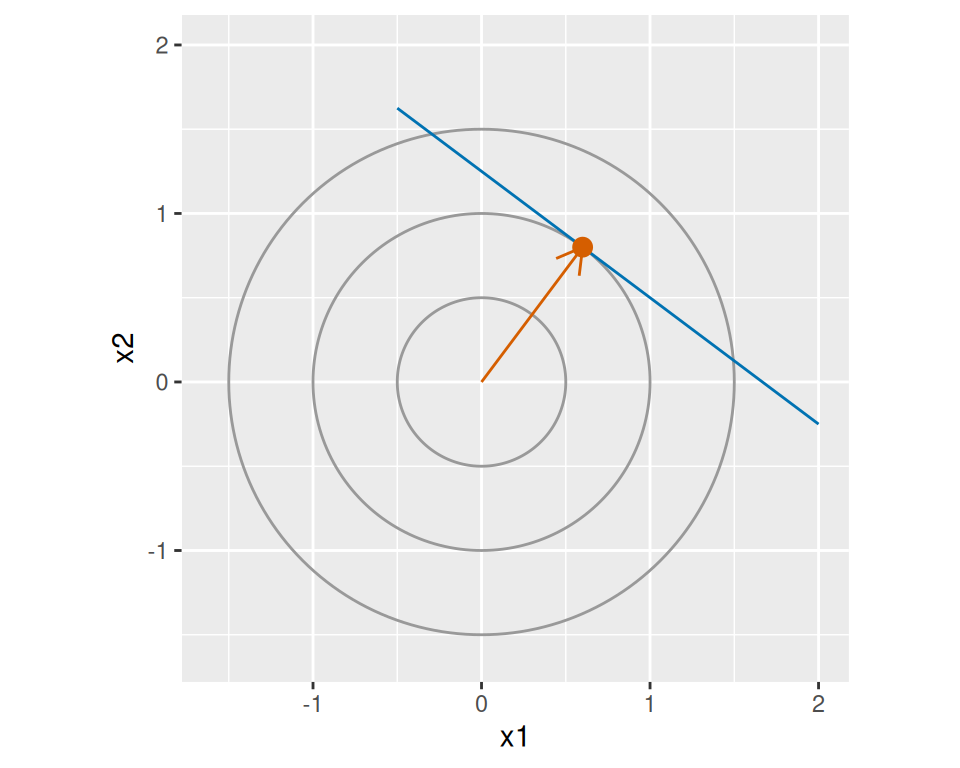
Example 5 (The closest point on a line to the origin) Minimize \(x_1^2 + x_2^2\) subject to \(3 x_1 + 4 x_2 = 5\). In the form of Theorem 1, \(x_1^2 + x_2^2 = \tfrac{1}{2}\,{\mathord{\smash[b]{\underset{\raise.3ex\hbox{$\scriptstyle\sim$}}{x}}\vphantom{x}}}^{\top} (2 \mathbf{I}_2) \mathord{\smash[b]{\underset{\raise.3ex\hbox{$\scriptstyle\sim$}}{x}}\vphantom{x}}\), so \(\mathbf{S} = 2 \mathbf{I}_2\), \(\mathbf{A} = {(3, 4)}^{\top}\) (\(p = 2\), \(m = 1\)) and \(\mathord{\smash[b]{\underset{\raise.3ex\hbox{$\scriptstyle\sim$}}{b}}\vphantom{b}} = [5]\). The hypotheses hold: \(2 \mathbf{I}_2\) is positive definite, and the single column \({(3, 4)}^{\top}\) is nonzero, so it is linearly independent. Also \(\mathbf{S}^{-1} = \tfrac{1}{2} \mathbf{I}_2\). Then, from the formulas of Theorem 1,

\[ \begin{aligned} \mathbf{M} &= {\mathbf{A}}^{\top}\,\tfrac{1}{2} \mathbf{I}_2\,\mathbf{A} \\ &= \tfrac{1}{2}\,(3^2 + 4^2) \\ &= \tfrac{25}{2}, \\ \mathord{\smash[b]{\underset{\raise.3ex\hbox{$\scriptstyle\sim$}}{x}}\vphantom{x}}^* &= \tfrac{1}{2} \mathbf{I}_2 \begin{bmatrix} 3 \\ 4 \end{bmatrix} \mathopen{}\left(\tfrac{2}{25}\right)\mathclose{} (5) \\ &= \tfrac{5}{25} \begin{bmatrix} 3 \\ 4 \end{bmatrix} \\ &= \begin{bmatrix} 0.6 \\ 0.8 \end{bmatrix}, \\ \mathord{\smash[b]{\underset{\raise.3ex\hbox{$\scriptstyle\sim$}}{\lambda}}\vphantom{\lambda}}^* &= -\mathopen{}\left(\tfrac{2}{25}\right)\mathclose{} (5) \\ &= -0.4, \\ f(\mathord{\smash[b]{\underset{\raise.3ex\hbox{$\scriptstyle\sim$}}{x}}\vphantom{x}}^*) &= \tfrac{1}{2} (5) \mathopen{}\left(\tfrac{2}{25}\right)\mathclose{} (5) \\ &= 1. \end{aligned} \]

Checks:

• the constraint:

  \[ \begin{aligned} 3 (0.6) + 4 (0.8) &= 1.8 + 3.2 \\ &= 5; \end{aligned} \]

• the first block of Equation 2:

  \[ \begin{aligned} \mathbf{S} \mathord{\smash[b]{\underset{\raise.3ex\hbox{$\scriptstyle\sim$}}{x}}\vphantom{x}}^* + \mathbf{A} \mathord{\smash[b]{\underset{\raise.3ex\hbox{$\scriptstyle\sim$}}{\lambda}}\vphantom{\lambda}}^* &= {(1.2, 1.6)}^{\top} + {(3, 4)}^{\top} (-0.4) \\ &= {(1.2, 1.6)}^{\top} - {(1.2, 1.6)}^{\top} \\ &= \mathord{\smash[b]{\underset{\raise.3ex\hbox{$\scriptstyle\sim$}}{0}}\vphantom{0}}_{2 \times 1}; \end{aligned} \]

• the value:

  \[ \begin{aligned} 0.6^2 + 0.8^2 &= 0.36 + 0.64 \\ &= 1. \end{aligned} \]

Geometrically, \(\mathord{\smash[b]{\underset{\raise.3ex\hbox{$\scriptstyle\sim$}}{x}}\vphantom{x}}^*\) is the point of the line nearest the origin, at distance \(1\).

ll_theta_ll <- seq(0, 2 * pi, length.out = 201)
ll_radii_ll <- c(0.5, 1, 1.5)
ll_circles_ll <- expand.grid(theta = ll_theta_ll, radius = ll_radii_ll)
ll_circles_ll$x1 <- ll_circles_ll$radius * cos(ll_circles_ll$theta)
ll_circles_ll$x2 <- ll_circles_ll$radius * sin(ll_circles_ll$theta)
ll_line_x1_ll <- c(-0.5, 2)
ll_line_x2_ll <- (5 - 3 * ll_line_x1_ll) / 4
ll_line_ll <- tibble::tibble(x1 = ll_line_x1_ll, x2 = ll_line_x2_ll)
ll_point_ll <- tibble::tibble(x1 = 0.6, x2 = 0.8)
ll_arrow_ll <- tibble::tibble(x = 0, y = 0, xend = 0.6, yend = 0.8)
ll_aes_ll <- ggplot2::aes(x1, x2)
ll_aes_circle_ll <- ggplot2::aes(x1, x2, group = radius)
ll_aes_arrow_ll <- ggplot2::aes(x = x, y = y, xend = xend, yend = yend)
ll_head_length_ll <- grid::unit(0.15, "inches")
ll_head_ll <- grid::arrow(length = ll_head_length_ll)
ll_lim_ll <- c(-1.6, 2)
ggplot2::ggplot() +
  ggplot2::geom_path(
    data = ll_circles_ll, mapping = ll_aes_circle_ll, colour = "grey60"
  ) +
  ggplot2::geom_line(
    data = ll_line_ll, mapping = ll_aes_ll, colour = "#0072B2"
  ) +
  ggplot2::geom_segment(
    data = ll_arrow_ll, mapping = ll_aes_arrow_ll,
    colour = "#D55E00", arrow = ll_head_ll
  ) +
  ggplot2::geom_point(
    data = ll_point_ll, mapping = ll_aes_ll, colour = "#D55E00", size = 3
  ) +
  ggplot2::coord_fixed(xlim = ll_lim_ll, ylim = ll_lim_ll) +
  ggplot2::labs(x = "x1", y = "x2")

import matplotlib.pyplot as plt
import numpy as np

ll_theta_ll = np.linspace(0, 2 * np.pi, 201)
fig, ax = plt.subplots(figsize=(5, 4), layout="constrained")
for ll_radius_ll in (0.5, 1, 1.5):
    ax.plot(ll_radius_ll * np.cos(ll_theta_ll),
            ll_radius_ll * np.sin(ll_theta_ll), color="grey")
ll_x1_ll = np.array([-0.5, 2])
ax.plot(ll_x1_ll, (5 - 3 * ll_x1_ll) / 4, color="#0072B2")
ax.annotate("", xy=(0.6, 0.8), xytext=(0, 0),
            arrowprops={"arrowstyle": "->", "color": "#D55E00"})
ax.plot(0.6, 0.8, "o", color="#D55E00", markersize=8)
ax.set_xlim(-1.6, 2)
#> (-1.6, 2.0)
ax.set_ylim(-1.6, 2)
#> (-1.6, 2.0)
ax.set_aspect("equal")
ax.set_xlabel("x1")
ax.set_ylabel("x2")
plt.show();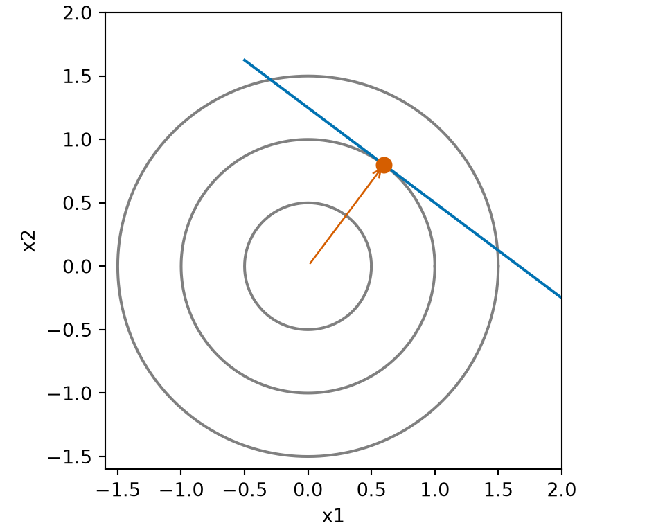

Figure 1: The level curves \(x_1^2 + x_2^2 = c\) of the objective (circles) and the constraint line \(3 x_1 + 4 x_2 = 5\). The line touches the circle \(c = 1\) at the minimizer \({(0.6, 0.8)}^{\top}\) (Example 5), and the arrow from the origin to that point points along the gradient there, which is perpendicular to the line.

• R
• Python

Example 6 (The hypotheses are needed)  

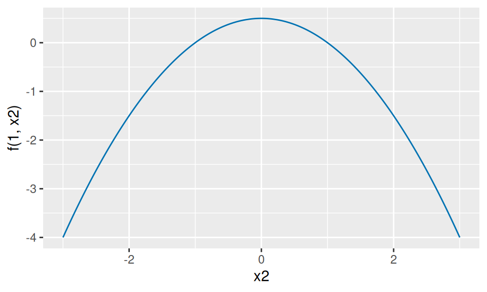
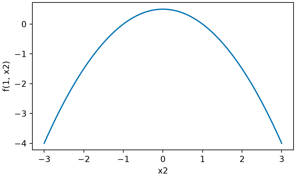
• If \(\mathbf{S}\) is not positive definite there may be no minimizer: with \(\mathbf{S} = \begin{bmatrix} 1 & 0 \\ 0 & -1 \end{bmatrix}\) and the constraint \(x_1 = 1\) (\(\mathbf{A} = {(1, 0)}^{\top}\), \(\mathord{\smash[b]{\underset{\raise.3ex\hbox{$\scriptstyle\sim$}}{b}}\vphantom{b}} = [1]\)), \(f(1, x_2) = \tfrac{1}{2} (1 - x_2^2)\) decreases without bound as \(x_2\) grows.

• If the columns of \(\mathbf{A}\) are dependent, \(\mathbf{M}\) is not invertible: with \(\mathbf{S} = \mathbf{I}_2\) and \(\mathbf{A} = \begin{bmatrix} 1 & 1 \\ 1 & 1 \end{bmatrix}\),

  \[ \begin{aligned} \mathbf{M} &= {\mathbf{A}}^{\top} \mathbf{A} \\ &= \begin{bmatrix} 2 & 2 \\ 2 & 2 \end{bmatrix}, \end{aligned} \]

  whose columns are equal. So \(\mathbf{M} {(1, -1)}^{\top} = \mathord{\smash[b]{\underset{\raise.3ex\hbox{$\scriptstyle\sim$}}{0}}\vphantom{0}}_{2 \times 1}\), and \(\mathbf{M}\) is not invertible, since a square matrix is invertible exactly when its null space is zero. The two constraints both read \(x_1 + x_2 = b_i\), so they have no solution at all when \(b_1 \ne b_2\). When \(b_1 = b_2\) a unique minimizer still exists,

  \[ \begin{aligned} x_1 &= x_2 \\ &= b_1 / 2, \end{aligned} \]

  but the formula of Theorem 1 cannot produce it.

qf_x2_qf <- seq(-3, 3, length.out = 201)
qf_curve_qf <- tibble::tibble(x2 = qf_x2_qf, f = 0.5 * (1 - qf_x2_qf^2))
ggplot2::ggplot(qf_curve_qf, ggplot2::aes(x2, f)) +
  ggplot2::geom_line(colour = "#0072B2") +
  ggplot2::labs(x = "x2", y = "f(1, x2)")

import matplotlib.pyplot as plt
import numpy as np

qf_x2_ax = np.linspace(-3, 3, 201)
fig, ax = plt.subplots(figsize=(5, 3), layout="constrained")
ax.plot(qf_x2_ax, 0.5 * (1 - qf_x2_ax**2), color="#0072B2")
ax.set_xlabel("x2")
ax.set_ylabel("f(1, x2)")
plt.show();

Figure 2: The first case of Example 6: with \(\mathbf{S} = \operatorname{diag}(1, -1)\), which is not positive definite, the value \(f(1, x_2)\) along the constraint \(x_1 = 1\) falls without bound as \(\mathopen{}\left|x_2\right|\mathclose{}\) grows, so this problem has no minimizer.

• R
• Python

Definition 9 (Sensitivity) Suppose a minimization problem (Definition 5) depends on a vector \(\mathord{\smash[b]{\underset{\raise.3ex\hbox{$\scriptstyle\sim$}}{b}}\vphantom{b}} \in \mathbb{R}^m\), and let \(f^*(\mathord{\smash[b]{\underset{\raise.3ex\hbox{$\scriptstyle\sim$}}{b}}\vphantom{b}})\) be its minimum value, as a function of \(\mathord{\smash[b]{\underset{\raise.3ex\hbox{$\scriptstyle\sim$}}{b}}\vphantom{b}}\). Where \(f^*\) has a gradient \(\frac{\partial}{\partial \mathord{\smash[b]{\underset{\raise.3ex\hbox{$\scriptstyle\sim$}}{b}}\vphantom{b}}} f^*(\mathord{\smash[b]{\underset{\raise.3ex\hbox{$\scriptstyle\sim$}}{b}}\vphantom{b}})\), that gradient is the sensitivity of the minimum value to \(\mathord{\smash[b]{\underset{\raise.3ex\hbox{$\scriptstyle\sim$}}{b}}\vphantom{b}}\): by the definition of a partial derivative, its entry \(i\) is the limit as a change in \(b_i\) alone shrinks to \(0\), of the resulting change in the minimum value divided by the change in \(b_i\).

Example 7 (The sensitivity of a one-point problem) Minimize \(x^2\) subject to \(x = b\), for a number \(b\). The feasible set (Definition 1) is \(\mathopen{}\left\{b\right\}\mathclose{}\), so the minimum value is \(f^*(b) = b^2\), and its sensitivity to \(b\) is \(\frac{d }{d b} f^*(b) = 2b\). At \(b = 3\) the sensitivity is \(6\): moving \(b\) from \(3\) to \(3.1\) raises the minimum value from \(9\) to \(9.61\), an increase of \(0.61\), close to \(6 \times 0.1 = 0.6\).

Corollary 1 (The multiplier is the sensitivity of the minimum value) In Theorem 1, write the minimum value as a function of \(\mathord{\smash[b]{\underset{\raise.3ex\hbox{$\scriptstyle\sim$}}{b}}\vphantom{b}}\), \(f^*(\mathord{\smash[b]{\underset{\raise.3ex\hbox{$\scriptstyle\sim$}}{b}}\vphantom{b}}) = \tfrac{1}{2}\,{\mathord{\smash[b]{\underset{\raise.3ex\hbox{$\scriptstyle\sim$}}{b}}\vphantom{b}}}^{\top} \mathbf{M}^{-1} \mathord{\smash[b]{\underset{\raise.3ex\hbox{$\scriptstyle\sim$}}{b}}\vphantom{b}}\). Its sensitivity to \(\mathord{\smash[b]{\underset{\raise.3ex\hbox{$\scriptstyle\sim$}}{b}}\vphantom{b}}\) (Definition 9) is

\[ \begin{aligned} \frac{\partial}{\partial \mathord{\smash[b]{\underset{\raise.3ex\hbox{$\scriptstyle\sim$}}{b}}\vphantom{b}}} f^*(\mathord{\smash[b]{\underset{\raise.3ex\hbox{$\scriptstyle\sim$}}{b}}\vphantom{b}}) &= \mathbf{M}^{-1} \mathord{\smash[b]{\underset{\raise.3ex\hbox{$\scriptstyle\sim$}}{b}}\vphantom{b}} \\ &= -\mathord{\smash[b]{\underset{\raise.3ex\hbox{$\scriptstyle\sim$}}{\lambda}}\vphantom{\lambda}}^*. \end{aligned} \]

Proof. \(\mathbf{M}^{-1}\) is symmetric and does not depend on \(\mathord{\smash[b]{\underset{\raise.3ex\hbox{$\scriptstyle\sim$}}{b}}\vphantom{b}}\), so derivative of a quadratic form applies with \(\mathbf{M}^{-1}\) in place of \(\mathbf{S}\):

\[ \begin{aligned} \frac{\partial}{\partial \mathord{\smash[b]{\underset{\raise.3ex\hbox{$\scriptstyle\sim$}}{b}}\vphantom{b}}} f^*(\mathord{\smash[b]{\underset{\raise.3ex\hbox{$\scriptstyle\sim$}}{b}}\vphantom{b}}) &= \tfrac{1}{2}\,\frac{\partial}{\partial \mathord{\smash[b]{\underset{\raise.3ex\hbox{$\scriptstyle\sim$}}{b}}\vphantom{b}}} \mathopen{}\left({\mathord{\smash[b]{\underset{\raise.3ex\hbox{$\scriptstyle\sim$}}{b}}\vphantom{b}}}^{\top} \mathbf{M}^{-1} \mathord{\smash[b]{\underset{\raise.3ex\hbox{$\scriptstyle\sim$}}{b}}\vphantom{b}}\right)\mathclose{} && \text{(constant multiple)} \\ &= \tfrac{1}{2} \mathopen{}\left(2 \mathbf{M}^{-1} \mathord{\smash[b]{\underset{\raise.3ex\hbox{$\scriptstyle\sim$}}{b}}\vphantom{b}}\right)\mathclose{} && \text{(derivative of a quadratic form)} \\ &= \mathbf{M}^{-1} \mathord{\smash[b]{\underset{\raise.3ex\hbox{$\scriptstyle\sim$}}{b}}\vphantom{b}} && \text{(simplify)} \\ &= -\mathord{\smash[b]{\underset{\raise.3ex\hbox{$\scriptstyle\sim$}}{\lambda}}\vphantom{\lambda}}^*. && \text{(definition of } \mathord{\smash[b]{\underset{\raise.3ex\hbox{$\scriptstyle\sim$}}{\lambda}}\vphantom{\lambda}}^* \text{)} \end{aligned} \]

Example 8 (Moving the line) In Example 5 with a general right side \(b\) in place of \(5\), \(\mathbf{M}^{-1} = \tfrac{2}{25}\) and

\[ \begin{aligned} f^*(b) &= \tfrac{1}{2} \mathopen{}\left(\tfrac{2}{25}\right)\mathclose{}\,b^2 \\ &= \tfrac{b^2}{25}, \end{aligned} \]

so \(\frac{d }{d b} f^*(b) = \tfrac{2b}{25}\). At \(b = 5\) this derivative is

\[ \begin{aligned} \tfrac{10}{25} &= 0.4 \\ &= -\lambda^*: \end{aligned} \]

moving the line \(3 x_1 + 4 x_2 = b\) outward by a small step \(\varepsilon\) in \(b\) raises the minimum value by about \(0.4\,\varepsilon\).

[1]

H. Zhou, “Optimization and multivariate calculus.” Lecture notes for Biostat 216, Mathematical Methods for Biostatistics, University of California, Los Angeles, 2024. Accessed: Oct. 05, 2026. [Online]. Available: https://ucla-biostat-216.github.io/2024fall/slides/13-optim/13-optim.html

[2]

Wikipedia contributors, “Feasible region — Wikipedia, the free encyclopedia.” 2026. Available: https://en.wikipedia.org/wiki/Feasible_region

[3]

Wikipedia contributors, “Mathematical optimization — Wikipedia, the free encyclopedia.” 2026. Available: https://en.wikipedia.org/wiki/Mathematical_optimization

[4]

Wikipedia contributors, “Lagrange multiplier — Wikipedia, the free encyclopedia.” 2026. Available: https://en.wikipedia.org/wiki/Lagrange_multiplier