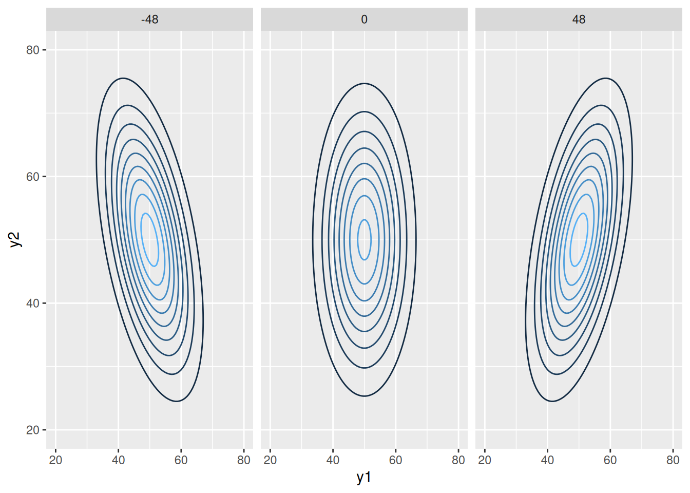
Chapter 7: The multivariate normal model
2016-11-10
5.1 Example: reading comprehension
We return to the example of two reading comprehension exams, given pre- and post-training.
Specifying prior
Mean
Assume the tests are designed such that people generally score 50 out of 100. Thus, our prior mean is \(\boldsymbol{\mu}_0 = (50, 50)^T\). Note that this implicitly assumes there is no effect of the training - the prior expectation of the post-training score is the same as the pre-training score.
Next, we need to specify the covariance of the prior expectation of the mean. Specifically, since the scores are bounded between 0 and 100, we should put little probability outside the \([0, 100]\) range (so a bell curve centered on 50 with 2 standard deviations \(\in [0, 100]\)). Then 1 standard deviation is 25 and the variance is thus 625.
Since the scores are both testing reading ability the scores are probably correlated. So if we want a prior correlation between \(\theta_1\) and \(\theta_2\) of 0.5, we need to solve the correlation equation
\[\begin{align} & 0.5 = \frac{\sigma_{1, 2}}{\sqrt{\sigma_1^2 \sigma_2^2}} \\ \implies& \sigma_{1, 2} = 0.5 \sqrt{625^2} = 312.5 \\ \end{align}\]
Therefore,
\[ \Lambda_0 = \begin{bmatrix} 625 & 312.5 \\ 312.5 & 625 \end{bmatrix} \]
Variance
We will use the guideline mentioned earlier for loosely centering our covariance matrix prior on \(\Lambda_0\). We’ll set \(\mathbf{S}_0^{-1} = \Lambda_0\) and \(\nu_0 = p + 2 = 4\).
Code
[R code]
# Note that this defines rmvnorm and rwish, but default
# implementations or packages are used here for real-world applications.
# Specifically MASS::mvrnorm (Modern Applied Statistics with S) is needed, and
# wishart comes default in newer R distributions with rWishart
source("Inline/chapter7.R")
# Try plotting
Y = Y.reading
ggplot(data.frame(Y.reading)) +
  geom_point(aes(x = pretest, y = posttest))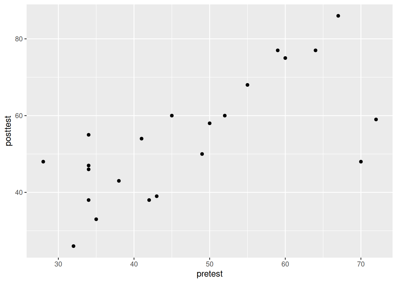
[R code]
# Gibbs sampling
library(MASS)
n = nrow(Y) # Number of observations
Sigma_0 = cov(Y) # Calculate covariance matrix; initial Sigma sample
# NOTE: This initial Sigma sample doesn't end up in the gibbs sample - we throw
# it away and start from scratch where sample 1 is the Theta based on Sigma_0, and
# the Sigma based on that new Theta
Sigma = Sigma_0
ybar = colMeans(Y) # Faster way of calculating column means

# TODO: Preallocate space for these instead of setting as NULL
THETA = NULL
SIGMA = NULL

# Also, inv = solve to make it more readable
inv = solve

set.seed(1)
for (s in 1:5000) {
  # Update theta
  # 1a. Compute params: Mu_n and Lambda_n from y_1, \dots, y_n and \Sigma^{(s)}
  # > Compute Lambda_n according to equation 7.4
  # Note: could cache inverse of priors
  Lambda_n = inv(inv(Lambda_0) + n * inv(Sigma))
  # > Compute Mu_n according to 7.5. Use Matrix mult
  # Note that he first term in 7.5 is Lambda_n
  Mu_n = Lambda_n %*% (inv(Lambda_0) %*% Mu_0 + n * inv(Sigma) %*% ybar)

  # 1b. Sample \theta^{(s + 1)} \sim multivariate normal mu_n, lambda_n
  # Now we know Lambda_n, Mu_n as implied by the known Sigma and data (p. 108).
  # Sample theta from multivariate normal (7.6, implied by 7.3)
  Theta = mvrnorm(n = 1, Mu_n, Lambda_n)

  # Known Theta. Now sample a new Sigma. NOTE: Old sigma gets thrown away!
  # 2a) Compute params for Sigma: Compute S_n from data and \theta^{(s + 1)}
  # i.e. Given the data and this Theta, we need to calculate the parameters that
  # define the full conditional distribution of \Sigma^{(s + 1)}
  # S_n according to p.112 first paragraph - not defined, but could be in 7.9
  # S_\theta is the residual sum of squares, defined in unlabeled equation after
  # 7.8
  # Use vectorized to avoid summation
  # Calculate residuals, then do sum of squares
  # Q: why t(Y)? just how elementwise works I guess
  resid = t(Y) - c(Theta)
  S_theta = resid %*% t(resid)
  S_n = S_0 + S_theta
  # 2b) Knowing the parameters for the full conditional distribution on Sigma
  # (inverse wishart with nu_0 and S_n known), sample
  # df = number of samples (degrees of freedom)
  # Don't forget to invert it afterwards (inverse wishart)
  # Weird thing is rWishart returns a weird list of arrays
  Sigma = inv(rWishart(1, nu_0 + n, inv(S_n))[, , 1])

  THETA = rbind(THETA, Theta)
  # Flatten sigma??
  SIGMA = rbind(SIGMA, c(Sigma))
}
Here are some associated calculations with this sample
[R code]
# Confidence interval for difference between post and pre test
quantile(THETA[, 2] - THETA[, 1], prob = c(0.025, 0.5, 0.975))
#>      2.5%       50%     97.5%
#>  1.454197  6.614914 11.663732

# Likelihood that the mean for the second test is greater than the mean for the
# 1st test
mean(THETA[, 2] > THETA[, 1])
#> [1] 0.9924

# Confidence interval for the correlation
CORR = apply(SIGMA, MARGIN = 1, FUN = function(row) {
  # indices 1 and 4 are correlation of dims 1 and 2
  # indices 2 is equal to index 3 is equal to covariance
  row[2] / sqrt(row[1] * row[4])
})
# Obviously there is a correlation
quantile(CORR, prob = c(0.025, 0.5, 0.975))
#>      2.5%       50%     97.5%
#> 0.4180072 0.6871101 0.8476477
We can also work with the posterior predictive distribution by sampling new pairs \((y_1, y_2)^{T(s)}\) from our samples of \(\boldsymbol{\theta}^{(s)}\) and \(\Sigma^{(s)}\):
Importantly, the probability of an individual having a higher post-test score than pre-test is much lower than the near-1 probability of the difference in mean test scores. It’s important to have clarified the difference between population means and individuals when drawing conclusions about your data.
6.2 Example
Let’s take a look at an example using a dataset with four health-related measurements on 200 women near Phoenix, Arizona. Notice that this dataset has missing values. We’ll assume that the data is missing at random, which is necessary for this analysis.
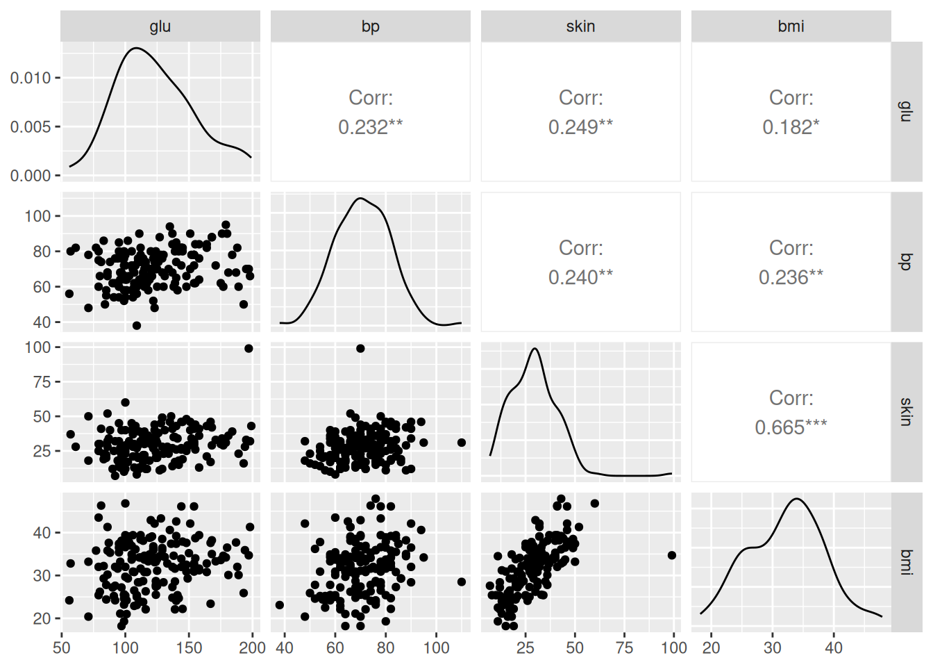
Gibbs sampling according to the 3-step scheme described above is implemented below. For priors, we set \(\boldsymbol{\mu}_0 = (120, 64, 26, 26)\) assuming we know these are the national averages of the health measurements. We then (waving our hands a little) select prior variances that keep these measurements mostly around zero and only lightly centered around our estimates.
[R code]
# Gibbs sampling
n = nrow(Y)
p = ncol(Y)
mu0 = c(120, 64, 26, 26)
sd0 = mu0 / 2
# Setting prior on covariance
L0 = matrix(.1, p, p)
diag(L0) = 1
L0 = L0 * outer(sd0, sd0)
print(L0)
#>      [,1]   [,2]  [,3]  [,4]
#> [1,] 3600  192.0  78.0  78.0
#> [2,]  192 1024.0  41.6  41.6
#> [3,]   78   41.6 169.0  16.9
#> [4,]   78   41.6  16.9 169.0

# Variance prior lightly concentrated, where nu0 > p is nu0 = p + 2
nu0 = p + 2
# Scale matrix - set to be the same as L0
S0 = L0

# Set starting values
Sigma = S0
Y.full = Y
O = 1 * (!is.na(Y))  # Get NOT NAs, coerce to int via * 1
for (j in 1:p) { # Looping through columns
  # For missing values in column, set to mean of the observed values
  mean.wo.na = mean(Y.full[, j], na.rm = TRUE)
  # Rows: all of those that are NA, and the jth column, set it to this mean
  Y.full[is.na(Y.full[, j]), j] = mean.wo.na
}

# Gibbs
THETA = SIGMA = Y.MISS = NULL
set.seed(1)
for (s in 1:1000) {
  # Update theta: step 1 of p.117 which is the same as previous
  ybar = colMeans(Y.full)
  Ln = inv(inv(L0) + n * inv(Sigma))
  mun = Ln %*% (inv(L0) %*% mu0 + n * inv(Sigma) %*% ybar)
  theta = mvrnorm(1, mun, Ln)

  # Update sigma: step 2 of p.117, same as previous
  resid = t(Y.full) - c(theta)
  Stheta = resid %*% t(resid)
  Sn = S0 + Stheta
  Sigma = inv(rWishart(1, nu0 + n, inv(Sn))[, , 1])

  # Update ymiss: step 3 of p.117, requires eqs 7.10, 7.11
  # Loop through rows of data (takes longer!!), need to sample rows individually
  # (independent) top of p.118
  for (i in 1:n) {
    # Skip if we already have it
    if (all(O[i, ] == 1)) {
      next
    }
    # Partition b = NA rows, a = present rows
    # Still works of a, b are empty, I presume
    oi = O[i, ]
    a = oi == 1
    b = oi == 0

    # Now we want to sample yb | ya, Sigma, Theta

    # \Sigma_{[a, a]}^{-1}, used in eqs 7.10 AND 7.11 (so calc once)
    iSa = inv(Sigma[a, a])
    # Calcualte \Sigma_{[b, a]}(\Sigma_{[a, a]})^{-1} used in 7.10 AND 7.11
    beta.j = Sigma[b, a] %*% iSa
    # Calculate Sigma.j (7.11). Start with covariacne matrix for the missing
    # vars, then influence by beta (decrease variance)
    Sigma.j = Sigma[b, b] - beta.j %*% Sigma[a, b]
    # Calculate theta.j (7.10). Start with standard theta, then change based on
    # residuals of other vals and what we wknow about covariances
    yi = Y.full[i, ]
    theta.j = theta[b] + beta.j %*% t(yi[a] - theta[a])

    # Now we have samples for subset of b. Preserver order, now sample
    Y.full[i, b] = mvrnorm(1, theta.j, Sigma.j)
  }

  # Concat
  THETA = rbind(THETA, theta)
  SIGMA = rbind(SIGMA, c(Sigma))
  Y.MISS = rbind(Y.MISS, Y.full[O == 0])
}

# Means and confidence intervals for posterior means
colnames(Y)
#> [1] "glu"  "bp"   "skin" "bmi"
colMeans(THETA)
#> [1] 123.51682  71.04978  29.38495  32.18491
apply(THETA, MARGIN = 2, FUN = function(d) quantile(d, prob = c(0.025, 0.5, 0.975)))
#>           [,1]     [,2]     [,3]     [,4]
#> 2.5%  118.7039 69.41573 27.62746 31.33561
#> 50%   123.5534 71.05000 29.39057 32.18047
#> 97.5% 127.8140 72.63692 31.05039 33.04161

# Sample correlation matrices
COR = array(dim = c(p, p, 1000))
for (s in 1:nrow(SIGMA)) {
  # It's in rows right now, refold into matrix
  Sig = matrix(SIGMA[s, ], nrow = p, ncol = p)
  # Calculate correlation matrix: (TODO: figure out how this works)
  COR[, , s] = Sig / sqrt(diag(Sig) %o% diag(Sig))
}

# Mean correlations from the correlation matrix samples. Can also calculate
# confidence intervals with quantile
apply(COR, MARGIN = c(1, 2), FUN = mean)
#>           [,1]      [,2]      [,3]      [,4]
#> [1,] 1.0000000 0.2236531 0.2475843 0.1888097
#> [2,] 0.2236531 1.0000000 0.2478914 0.2349531
#> [3,] 0.2475843 0.2478914 1.0000000 0.6510103
#> [4,] 0.1888097 0.2349531 0.6510103 1.00000007.2 7.3
a
[R code]
crab.mcmc = lapply(list('bluecrab' = bluecrab, 'orangecrab' = orangecrab), function(crab) {
  p = ncol(crab)
  n = nrow(crab)
  ybar = colMeans(crab)

  # Prior parameters

  mu0 = ybar
  lambda0 = s0 = cov(crab)
  nu0 = 4

  S = 10000
  THETA = matrix(nrow = S, ncol = p)
  SIGMA = array(dim = c(p, p, S))

  # Start with sigma sample
  sigma = s0

  # Gibbs sampling
  library(MASS)

  # Also, inv = solve to make it more readable
  inv = solve

  for (s in 1:S) {
    # Update theta
    lambdan = inv(inv(lambda0) + n * inv(sigma))
    mun = lambdan %*% (inv(lambda0) %*% mu0 + n * inv(sigma) %*% ybar)
    theta = mvrnorm(n = 1, mun, lambdan)

    # Update sigma
    resid = t(crab) - c(theta)
    stheta = resid %*% t(resid)
    sn = s0 + stheta
    sigma = inv(rWishart(1, nu0 + n, inv(sn))[, , 1])

    THETA[s, ] = theta
    SIGMA[, , s] = sigma
  }

  list(theta = THETA, sigma = SIGMA)
})
b
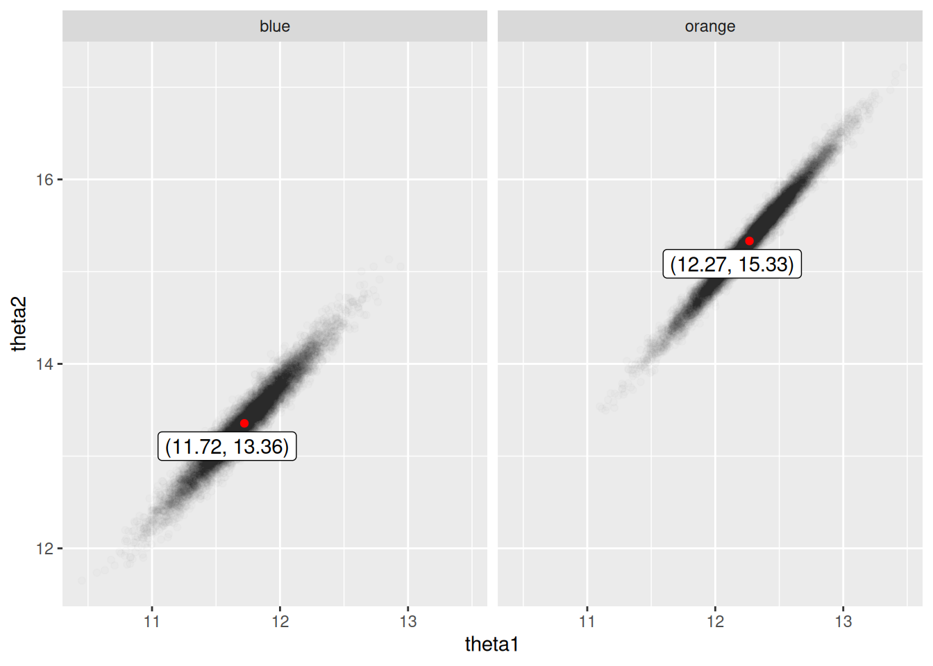
There is strong evidence that orange crabs tend to be larger in both measurements than blue crabs:
c
[R code]
bluecrab.cor = apply(crab.mcmc$bluecrab$sigma, MARGIN = 3, FUN = function(covmat) {
  covmat[1, 2] / (sqrt(covmat[1, 1] * covmat[2, 2]))
})
orangecrab.cor = apply(crab.mcmc$orangecrab$sigma, MARGIN = 3, FUN = function(covmat) {
  covmat[1, 2] / (sqrt(covmat[1, 1] * covmat[2, 2]))
})
cor.df = data.frame(species = c(rep('blue', length(bluecrab.cor)), rep('orange', length(orangecrab.cor))),
                    cor = c(bluecrab.cor, orangecrab.cor))
ggplot(cor.df, aes(x = cor, fill = species)) +
  geom_density(alpha = 0.5) +
  scale_fill_manual(values = c('blue', 'orange'))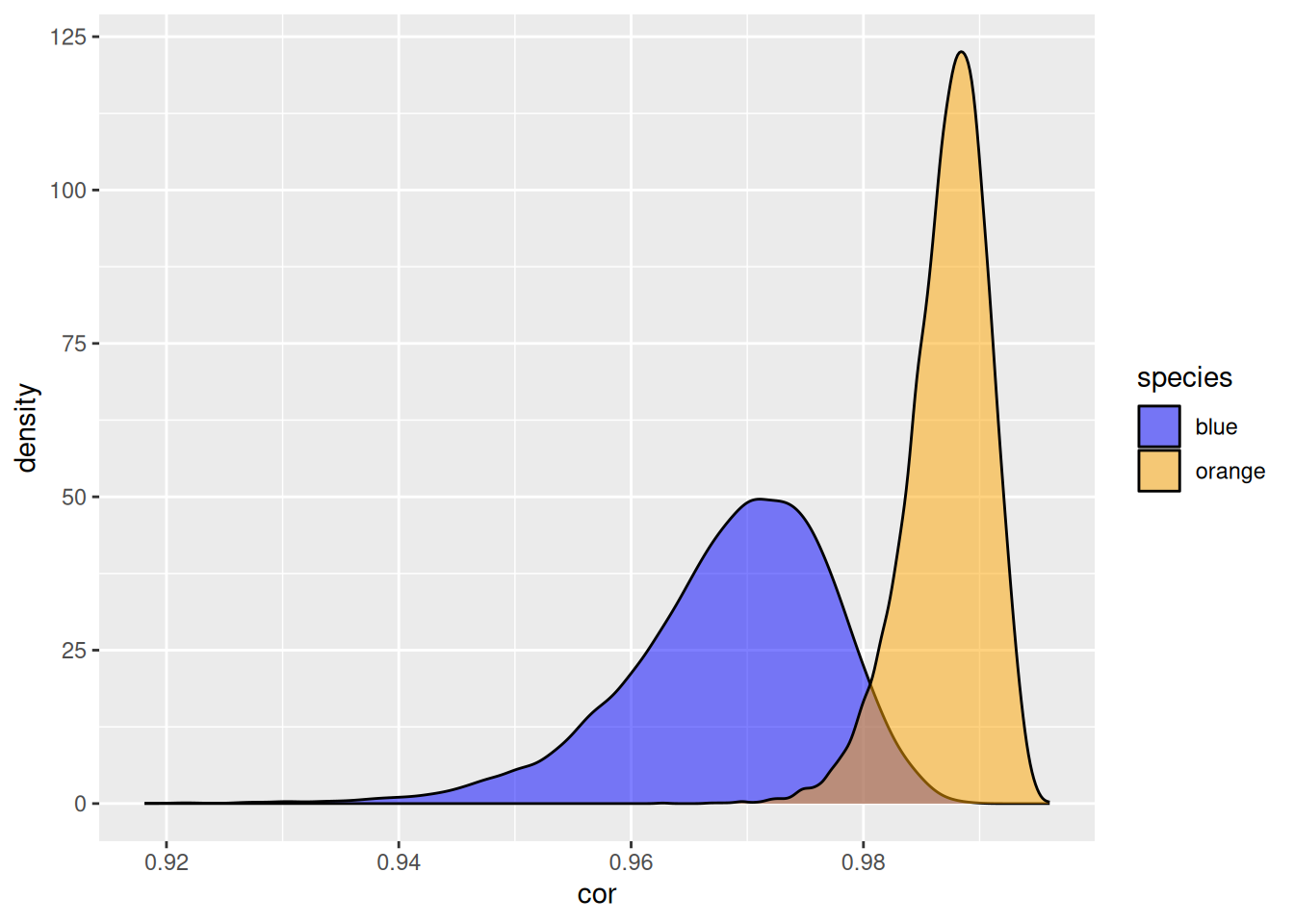
The orange crab species appears to have a much higher correlation between its two measurements than the blue crab species.
7.3 7.4
a
With typical intuitions about life expectancy and age of marriage, I suspect that the ages of most of the married couples will fall between 25 and 80. There may be slight age differences among men and women, but not enough to warrant encoding in the prior. Thus \(\boldsymbol{\mu}_0 = ((25 + 80) / 2, (25 + 80) / 2) = (52.5, 52.5)^T\) is set.
A semiconjugate prior distribution is chosen in this case, as it seems intuitive that there are fewer married couples at ages 25 and 80 than there are married couples around age 50, thus justifying a bell curve centered around \(52.5\) with variance \(13.75^2 \approx 189\) such that approximately 95% of the prior falls within the range \((25, 80)\).
The ages of the couples are expected to be quite tightly correlated, so knowing the above variance, a prior correlation of \(0.75\) is targeted. Solving the correlation equation gives
\[\begin{align} & 0.75 = \frac{\sigma_{1, 2}}{189} \\ \implies& \sigma_{1, 2} = 141.75 \end{align}\]
Thus \[\Lambda_0 = \begin{bmatrix} 189 & 141.75 \\ 141.75 & 189 \end{bmatrix} \] is set.
Like previous problems, for the variance, \(\mathbf{S}_0^{-1} = \Lambda_0\) and \(\nu_0 = p + 2 = 4\) are set. Note that this only loosely centers the covariance matrix prior on \(\Lambda_0\), representing a conservative approach in terms of belief in the variance and the correlation between the ages.
b
The wording of the question is interesting - the assumption is to sample a fixed \(\boldsymbol{\theta}, \Sigma\) and from there sample \(100\) points all with the same parameters. An alternative approach would be to sample a new data point for each sample of \(\boldsymbol{\theta}, \Sigma\).
In fact, because of that wording, \(\nu_0 = p + 2 = 4\) was originally set to loosely center the prior. But given that this variance will often produce uncorrelated prior predictive datasets, \(\nu_0\) is increased slightly.
After increasing \(\nu_0\), the posterior predictive datasets appear satisfactory.
[R code]
N = 100
S = 12

Y_preds = lapply(1:S, function(s) {
  # Sample THETA according to prior
  theta = mvrnorm(n = 1, mu0, lambda0)
  sigma = inv(rWishart(1, nu0, inv(s0))[, , 1])
  Y_s = mvrnorm(n = 100, theta, sigma)
  data.frame(Y1 = Y_s[, 1], Y2 = Y_s[, 2], dataset = s)
})

Y_comb = do.call(rbind, Y_preds)

ggplot(Y_comb, aes(x = Y1, y = Y2)) +
  geom_point() +
  facet_wrap(~ dataset)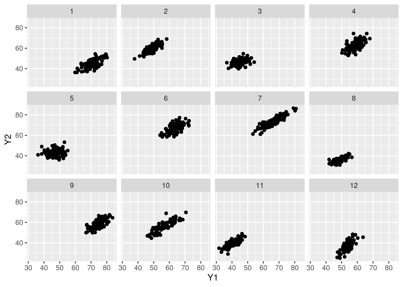
c
[R code]
S = 10000

# Reuse this since we'll need to specify different priors
do_mcmc = function(Y, mu0, lambda0, s0, nu0) {
  ybar = colMeans(Y)
  p = ncol(Y)
  n = nrow(Y)

  THETA = matrix(nrow = S, ncol = p)
  SIGMA = array(dim = c(p, p, S))

  # Start with sigma sample
  sigma = cov(Y)

  # Gibbs sampling

  # Also, inv = solve to make it more readable
  inv = solve

  for (s in 1:S) {
    # Update theta
    lambdan = inv(inv(lambda0) + n * inv(sigma))
    mun = lambdan %*% (inv(lambda0) %*% mu0 + n * inv(sigma) %*% ybar)
    theta = mvrnorm(n = 1, mun, lambdan)

    # Update sigma
    resid = t(Y) - c(theta)
    stheta = resid %*% t(resid)
    sn = s0 + stheta
    sigma = inv(rWishart(1, nu0 + n, inv(sn))[, , 1])

    THETA[s, ] = theta
    SIGMA[, , s] = sigma
  }

  list(theta = THETA, sigma = SIGMA)
}

my_prior_mcmc = do_mcmc(agehw, mu0, lambda0, s0, nu0)
THETA = my_prior_mcmc$theta
SIGMA = my_prior_mcmc$sigma

# For reuse later
print_quantiles = function(THETA, SIGMA) {
  print("Husband")
  print(quantile(THETA[, 1], probs = c(0.025, 0.5, 0.975))) # Husband
  print("Wife")
  print(quantile(THETA[, 2], probs = c(0.025, 0.5, 0.975))) # Wife
  cors = apply(SIGMA, MARGIN = 3, FUN = function(covmat) {
    covmat[1, 2] / (sqrt(covmat[1, 1] * covmat[2, 2]))
  })
  print("Correlation")
  print(quantile(cors, probs = c(0.025, 0.5, 0.975)))
}

print_quantiles(THETA, SIGMA)
#> [1] "Husband"
#>     2.5%      50%    97.5%
#> 42.01685 44.52494 47.03880
#> [1] "Wife"
#>     2.5%      50%    97.5%
#> 38.60299 40.99994 43.42255
#> [1] "Correlation"
#>      2.5%       50%     97.5%
#> 0.8615416 0.9028502 0.9321153
d
Exercise 7.2 has not been completed, but doing Jeffreys’ prior and a “diffuse prior” below will still be helpful to see what effect prior information has.
i
[R code]
THETA = matrix(nrow = S, ncol = p)
SIGMA = array(dim = c(p, p, S))

# Start with sigma sample
sigma = cov(Y)

# Gibbs sampling

# Also, inv = solve to make it more readable
inv = solve

for (s in 1:S) {
  # Update theta
  theta = mvrnorm(n = 1, ybar, sigma / n)

  # Update sigma
  resid = t(Y) - c(theta)
  stheta = resid %*% t(resid)
  sigma = inv(rWishart(1, n + 1, inv(stheta))[, , 1])

  THETA[s, ] = theta
  SIGMA[, , s] = sigma
}

print_quantiles(THETA, SIGMA)
#> [1] "Husband"
#>     2.5%      50%    97.5%
#> 41.73803 44.42889 47.15085
#> [1] "Wife"
#>     2.5%      50%    97.5%
#> 38.37376 40.91439 43.48397
#> [1] "Correlation"
#>      2.5%       50%     97.5%
#> 0.8608382 0.9038100 0.9347940
ii
Unit information prior (skipping)
iii
[R code]
mu0 = rep(0, p)
lambda0 = 10^5 * diag(p)
s0 = 1000 * diag(p)
nu0 = 3
diffuse_mcmc = do_mcmc(agehw, mu0, lambda0, s0, nu0)
print_quantiles(diffuse_mcmc$theta, diffuse_mcmc$sigma)
#> [1] "Husband"
#>     2.5%      50%    97.5%
#> 41.67960 44.41405 47.18645
#> [1] "Wife"
#>     2.5%      50%    97.5%
#> 38.32275 40.88109 43.51451
#> [1] "Correlation"
#>      2.5%       50%     97.5%
#> 0.7931776 0.8552845 0.8996432
e
It doesn’t really seem like the prior information matters because the sample size is so large. Regardless of whether the prior is informative, the quantiles and correlations end up quite similar. Maybe the diffuse prior is slightly different, but it’s not a big difference.
If a smaller sample size is used, this may be different. The following shows what happens when the dataset is truncated to the first 25 variables and rerun with the informative prior and the diffuse prior:
Informative prior
[R code]
mu0 = rep(52.5, p)
lambda0 = s0 = rbind(c(189, 141.75), c(141.75, 189))
# nu0 = p + 2
nu0 = p + 2 + 10
my_prior_mcmc_short = do_mcmc(agehw[1:25, ], mu0, lambda0, s0, nu0)
print_quantiles(my_prior_mcmc_short$theta, my_prior_mcmc_short$sigma)
#> [1] "Husband"
#>     2.5%      50%    97.5%
#> 40.96477 45.37803 49.83724
#> [1] "Wife"
#>     2.5%      50%    97.5%
#> 38.41850 43.04898 47.77481
#> [1] "Correlation"
#>      2.5%       50%     97.5%
#> 0.8418117 0.9136244 0.9540250
Diffuse prior
[R code]
mu0 = rep(0, p)
lambda0 = 10^5 * diag(p)
s0 = 1000 * diag(p)
nu0 = 3
diffuse_mcmc_short = do_mcmc(agehw[1:25, ], mu0, lambda0, s0, nu0)
print_quantiles(diffuse_mcmc_short$theta, diffuse_mcmc_short$sigma)
#> [1] "Husband"
#>     2.5%      50%    97.5%
#> 39.07635 45.12302 51.00340
#> [1] "Wife"
#>     2.5%      50%    97.5%
#> 36.53189 42.74457 48.81278
#> [1] "Correlation"
#>      2.5%       50%     97.5%
#> 0.5427696 0.7613713 0.8823101
In this case, the effect of the prior on correlation especially is easily observed. The correlation for the diffuse prior is quite low, as it is being dragged towards nothing.