Chapter 6: Posterior approximation with the Gibbs sampler

Jesse Mu

2016-11-04

1 A semiconjugate prior distribution

In Chapter 5, we performed two-parameter inference by decomposing the prior \(p(\theta, \sigma^2) = p(\theta \mid \sigma^2) p(\sigma^2)\). So our prior distribution on \(\theta\) relates to the variance \(\sigma^2\):

\[ \theta \mid \sigma^2 \sim \mathcal{N}(\mu_0, \sigma^2 / \kappa_0) \]

However, consider that we may want to decouple the priors of the two parameters. This allows flexibility with specification of the prior (initial estimate and confidence) of either parameter.

Consider the midge wing example: we picked a prior on \(\theta\) that was centered around 1.9 (our prior expectation) but with most of its mass above 0, since wing lengths cannot be above 0. We can’t freely do this from what we know in section 5 (i.e. setting \(\tau_0^2 = \sigma^2 / \kappa_0\)). Alternatively, we can set \(\tau_0^2\) to be whatever we want, but then there is no longer a known form of the joint posterior

\[ p(\theta, \sigma^2 \mid y_1, \dots, y_n) \propto p(\theta, \sigma^2) \times p(y_1, \dots, y_n \mid \theta, \sigma^2) \]

that can easily be sampled from. However, as it turns out, the full conditionals \(p(\theta \mid \sigma^2, y_1, \dots, y_n)\) and \(p(\sigma^2 \mid \theta, y_1, \dots, y_n)\) are easy to specify, as when evaluating the formulas, we can simply disregard the other fixed parameter as a constant, leading to known posterior distributions. A technicue called Gibbs sampling allows us to take advantage of this by constructing a sampler that approximates the (unknown) joint distribution by sampling iteratively from the (known) full conditional distributions.

2 Discrete approximations

Why posterior densities are hard to calculate for nonconjugate priors using Bayes rule?

\[ \begin{aligned} p(\boldsymbol{\theta} \mid \mathbf{y}) &= \frac{p(\mathbf{y} \mid \theta) p(\boldsymbol{\theta})}{\int p(\mathbf{y} \mid \boldsymbol{\theta}') p(\boldsymbol{\theta}') \; d\boldsymbol{\theta}'} \end{aligned} \]

The numerator here is often easy to calculate, but the denominator is often prohibitively hard to compute. When the numerator is not known to be proportional to a known probability distribution, we can’t get the full joint density without the denominator.

Notice however that we can still evaluate relative probabilites of \(\boldsymbol{\theta}_a\) and \(\boldsymbol{\theta}_b\), as their ratio cancels out the integral. More generally, we can create a discrete approximation of the probabilities by evaluating the numerator of this density for values of \(\boldsymbol{\theta}\) across an \(n\)-dimensional grid, then dividing each of these unnormalized densities by the sum of the entire grid.

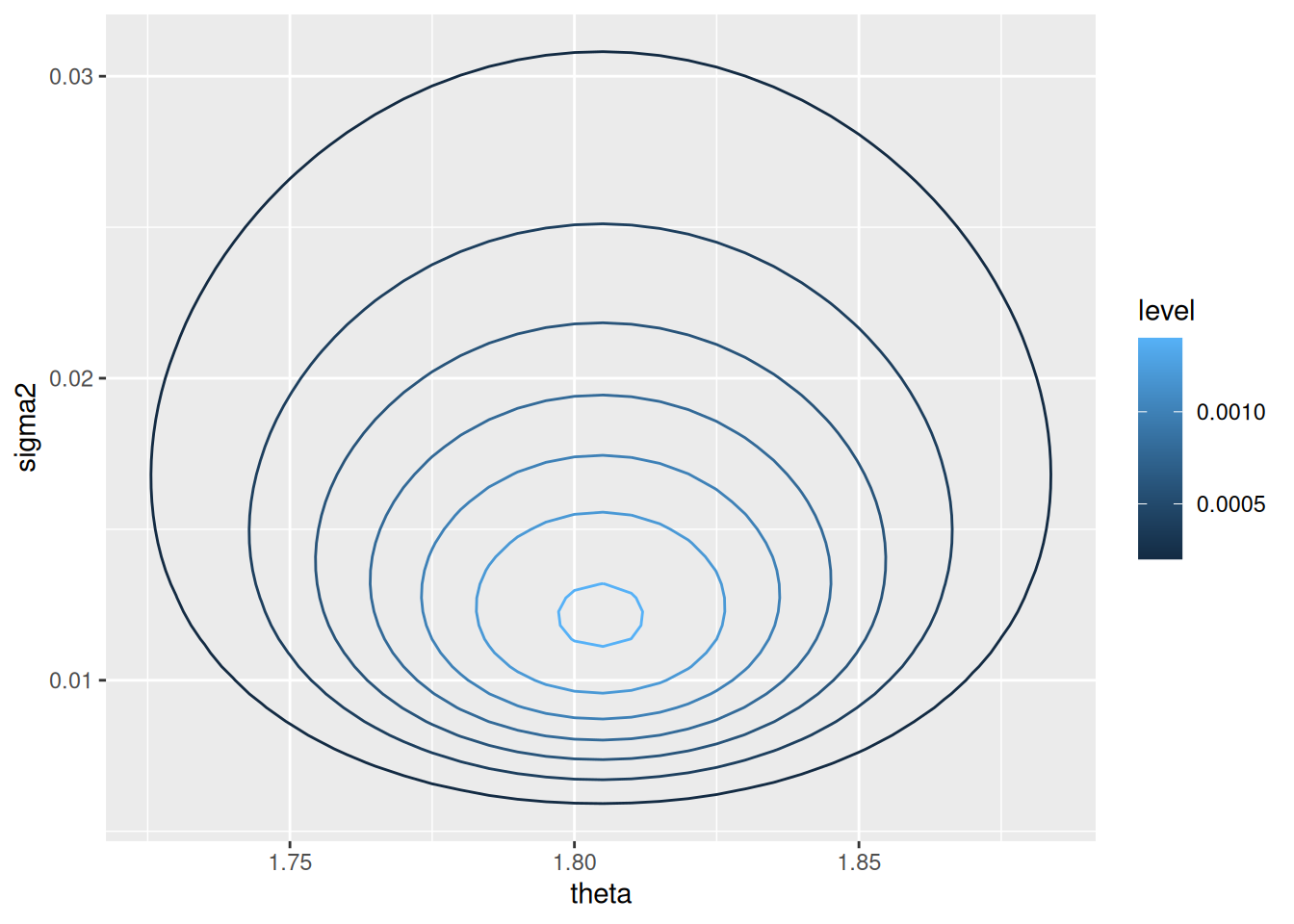
Funnily, this is pretty much what I have been doing in the past chapters when plotting heatmaps:

y = c(1.64, 1.70, 1.72, 1.74, 1.82, 1.82, 1.82, 1.90, 2.08)

n = length(y)
ybar = mean(y)
s2 = var(y)

# Prior

mu0 = 1.9
# Tau chosen such that most of the mass of the normal distribution > 0
t20 = 0.95^2
s20 = 0.01
nu0 = 1

Theta = seq(1.505, 2, length = 100)
Sigma2 = seq(0.005, 0.05, length = 100)

# This calculates p(sigma2, theta, y_1, \dots, y_n)
library(invgamma)
post.func = Vectorize(function(theta, sigma2) {
  dnorm(theta, mu0, sqrt(t20)) *
    dinvgamma(sigma2, nu0 / 2, s20 * nu0 / 2) *
    prod(dnorm(y, theta, sqrt(sigma2)))
})

d = outer(Theta, Sigma2, post.func)
rownames(d) = Theta
colnames(d) = Sigma2
d = d / sum(d)

df = as.data.frame(d) |>
  tibble::rownames_to_column('theta') |>
  pivot_longer(cols = -theta, names_to = 'sigma2', values_to = 'density') |>
  mutate(theta = as.numeric(theta), sigma2 = as.numeric(sigma2))

ggplot(df, aes(x = theta, y = sigma2, z = density)) +
  geom_contour(aes(color = ..level..))

3 Sampling from the conditional distributions

Again, to proceed with Gibbs sampling, we simply need to calculate the full conditional distributions of the parameters. We already computed the full conditional for \(\theta \mid \sigma^2, y_1, \dots, y_n\) in 5.2. For \(\theta \mid \mathcal{N}(\mu_0, \tau_0^2)\), then \(\theta \mid \sigma^2, y_1, \dots, y_n \sim \mathcal{N}(\mu_n, \tau_n^2)\), where \(\mu_n\) and \(\tau_n^2\) are not reproduced here (see 5.2).

Now we find the full conditional for \(\sigma^2\) using the exact same method as in 5.2:

\[ \begin{aligned} p(\sigma^2 \mid \theta, y_1, \dots, y_n) &\propto \left[(\sigma^2)^{-n/2} \text{exp}\left(-\frac{1}{2\sigma^2} \sum_{i = 1}^n (y_i - \theta)^2 \right) \right] \times \left[ (\sigma^2)^{- \nu_0 / 2 - 1} \text{exp} \left(-\frac{\sigma_0^2 \nu_0 / 2}{\sigma^2} \right) \right] \\ &\propto (\sigma^2)^{-(\nu_0 + 1) / 2 - 1} \times \text{exp}\left(-\frac{1}{\sigma^2} \times \frac{1}{2}\left(\sigma_0^2 \nu_0 + \sum_{i=1}^{n} (y_i - \theta)^2 \right) \right) \\ \end{aligned} \]

So \(\sigma^2 \sim \text{inverse-gamma}(\nu_n / 2, \nu_n \sigma_n^2(\theta) / 2)\), and \(\tilde{\sigma^2} \sim \text{gamma}(\cdot, \cdot))\), with the parameters:

• \(\nu_n = \nu_0 + n\)
• \(\sigma_n^2(\theta) = (\sigma_0^n \nu_0 + n s_n^2(\theta)) / \nu_n\)

We denote \(\sigma_n^2(\theta)\), \(s_n^2(\theta)\) to indicate that \(\sigma_n^2\) is dependent on \(\theta\) which is assumed known.

A shortcut for thinking about full conditionals, instead of explicitly decomposing the probability according to Bayes rule each time, is to write the numerator of the full joint posterior \(p(\boldsymbol{\theta} \mid \mathbf{y})\). Then, if you are interested in the full conditional of \(p(\theta_i \mid \mathbf{y})\), simply evaluate the full joint posterior while treating all \(\theta_j\) for \(j \neq i\) as constants (and thus discardable to maintain proportionality). This is used in later chapters (e.g. 8.3.1)

4 Gibbs sampling

From this, Gibbs sampling proceeds as follows:

Begin with start values \(\theta_i^{(0)}\) for all \(i\). Usually these can be standard naive estimates of the parameters. Also, you technically only have to have start values for all but one parameter, because now…

• (WOLOG) Sample \(\theta_1^{(1)} \sim p(\theta_1 \mid \theta_2^{(0)}, \dots, \theta_n^{(0)}, \dots)\) (the full conditional)
• Similarly, sample \(\theta_2^{(1)} \sim p(\theta_2 \mid \dots)\), \(\theta_3^{(1)} \sim p(\theta_3 \mid \dots)\).
• \(\boldsymbol{\theta}^{(1)} = \begin{pmatrix} \theta_1^{(1)} & \cdots & \theta_n^{(1)} \end{pmatrix}\) is your first Gibbs sample.
• Given Gibbs sample \(\boldsymbol{\theta}^{(s)}\), for further samples, sample each \(\theta_i^{(s + 1)}\) individually as before, conditioning on the \(\theta_i^{(s)}\) of the previous gibbs sampling \(\boldsymbol{\theta}^{(s)}\) and the new samples \(\theta_i^{(s + 1)}\) as they are received. Then \(\boldsymbol{\theta}^{(s + 1)} = \begin{pmatrix} \theta_1^{(s + 1)} & \cdots & \theta_n^{(s + 1)} \end{pmatrix}\) is the \(s + 1\)th Gibbs sample.

Notice that the \(s + 1\)th sample is only conditionally dependent on the \(s\)th sample, hence the term “Markov Chain Monte Carlo”. Once these samples are obtained, you can treat them like a standard Monte Carlo sample, and compute all of the desired quantities.

The following is an example for our midge length data:

S = 1000
PHI = matrix(nrow = S, ncol = 2)
PHI[1, ] = phi = c(ybar, 1 / s2) # Start with sample mean + variance

set.seed(1) # Reproducibility
# Should use a for loop, as there are variables we need to keep track of through
# iterations
for (s in 2:S) {
  # Sample theta based on \sigma^2 (phi[2])
  # According to normal(\mu_n, \tau^2_n) where \mu_n and \tau^2_n are as below
  mun = (mu0 / t20 + n * ybar * phi[2]) / (1/t20 + n * phi[2])
  t2n = 1 / (1 / t20 + n * phi[2])
  phi[1] = rnorm(1, mun, sqrt(t2n))

  # Sample 1/sigma^2 based on \theta
  nun = nu0 + n
  s2n = (nu0 * s20 + (n - 1) * s2 + n * (ybar - phi[1])^2) / nun
  # This posterior distribution: inverse-gamma(\nu_n / 2, \sigma^2_n(\theta)
  # \nu_n / 2)
  phi[2] = rgamma(1, nun / 2, s2n * nun / 2)

  PHI[s, ] = phi
}

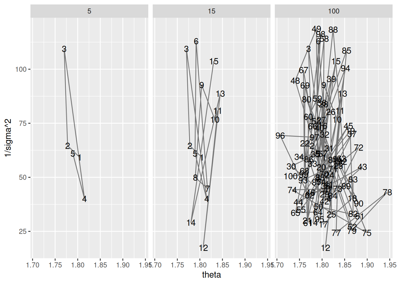
The following are plots of 5, 15, and 100 consecutive Gibbs samples for \(\theta\) and \(\tilde{\sigma^2}\):

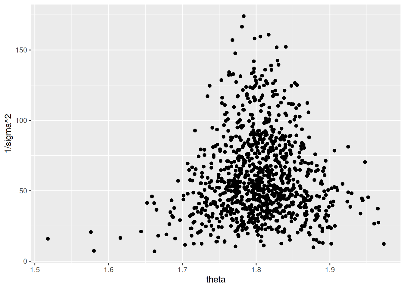
This is the scatterplot of all 1000 of our Gibbs samples:

ggplot(phi.df, aes(x = theta, y = `1/sigma^2`)) + geom_point()

Finally, some quantiles:

# CI for population mean - first column is theta
quantile(PHI[, 1], c(0.025, 0.5, 0.975))
#>     2.5%      50%    97.5% 
#> 1.707282 1.804348 1.901129
# CI for population precision, second column
quantile(PHI[, 2], c(0.025, 0.5, 0.975))
#>      2.5%       50%     97.5% 
#>  17.48020  53.62511 129.20020
# CI for population stddev, arbitrary function of second column
quantile(1 / sqrt(PHI[, 2]), c(0.025, 0.5, 0.975))
#>       2.5%        50%      97.5% 
#> 0.08797701 0.13655763 0.23918408

# For later
midge.df = phi.df

5 General properties of the Gibbs sampler

Under conditions that will be met for our models, like the law of large numbers for standard monte carlo sampling, a sufficient number of Gibbs samples approaches the target distribution. The question of course is how many samples is enough, which is covered in the next section.

Another important point is that Gibbs sampling is not a Bayesian model. These two concepts should be separated: Gibbs sampling is a general framework for “observing” the posterior probability distribution, whatever that distribution is.

6 Introduction to MCMC diagnostics

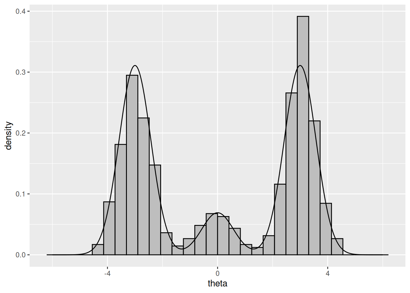
For an example of the importance of assessing convergence of Gibbs sampling, consider the following target distribution, a 45-10-45 mixture of \(\mathcal{N}(-3, 1/3), \mathcal{N}(0, 1/3), \mathcal{N}(3, 1/3)\):

A Gibbs sampler to obtain samples from this is:

# Gibbs sampling with S = 1000
S = 1000
PHI = matrix(nrow = S, ncol = 2)
# Let delta0 = 2 and theta0 = 0
PHI[1, ] = phi = c(2, 0)

set.seed(1) # Reproducibility
# Should use a for loop, as there are variables we need to keep track of through
# iterations
for (s in 2:S) {
  # Sample delta s+1 based on theta s
  probs = sapply(1:3, function(d) {
    PROB.DENS[d] * dnorm(phi[2], MU.DENS[d], sqrt(S2.DENS[d]))
  })
  probs = probs / sum(probs)
  phi[1] = sample.int(3, size = 1, prob = probs)

  # Sample theta s+1 based on delta (easy)
  phi[2] = rnorm(1, MU.DENS[phi[1]], sqrt(S2.DENS[phi[1]]))

  PHI[s, ] = phi
}

theta.mcmc = data.frame(PHI)
colnames(theta.mcmc) = c('delta', 'theta')
theta.mcmc$iteration = 1:nrow(theta.mcmc)

# How well does this work?
ggplot(theta.dist, aes(x = theta, y = density)) +
  geom_histogram(mapping = aes(x = theta, y = ..density..), data = theta.mcmc,
                 color = 'black', fill = 'grey') +
  geom_line()

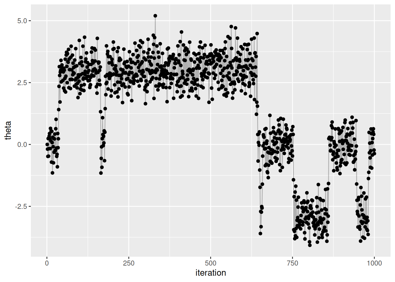
# Traceplot
ggplot(theta.mcmc, aes(x = iteration, y = theta)) +
  geom_point() +
  geom_line(alpha = 0.25)

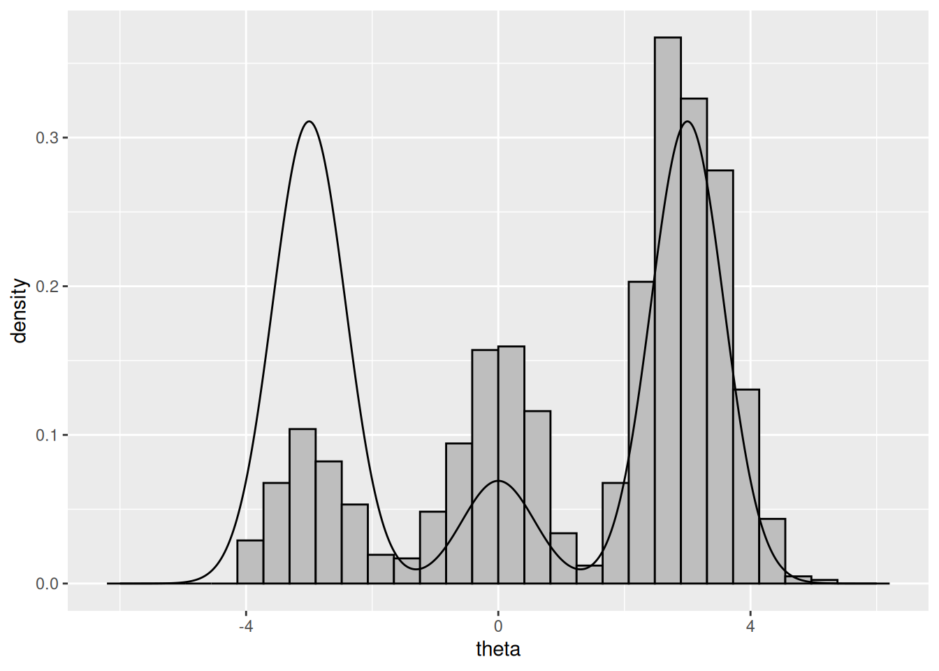
Notice that the histogram does not adequately approximate the distribution. Try changing the number of samples to 10000 or 100000, which should be better.

The problem is that since the sampler generates dependent samples, the sampler sticks in high probability regions for a long time. After sufficient samples, this balances out, but sometimes the number of samples required may be very large.

Getting it right

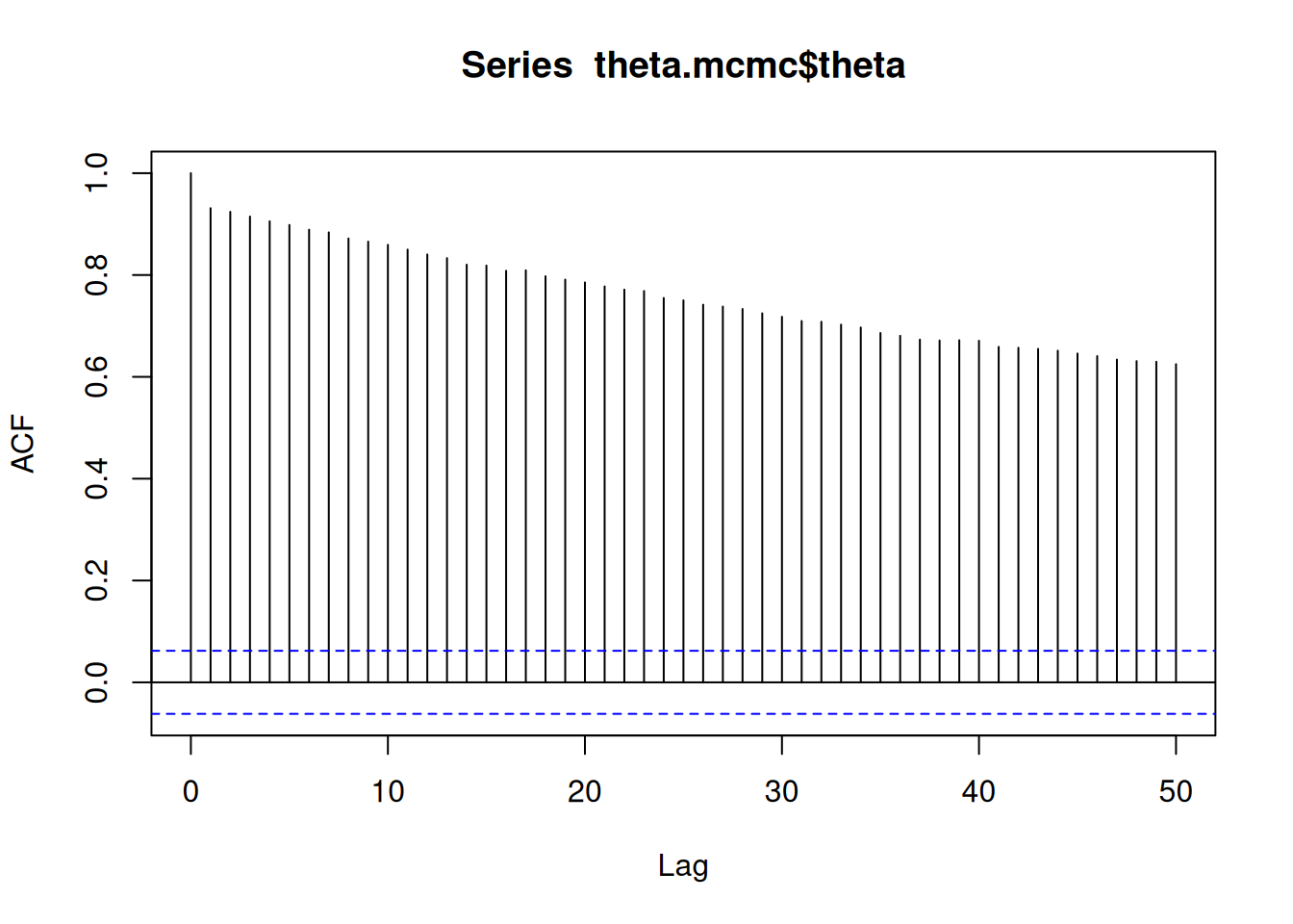
Estimate of MCMC depends on autocorrelation: how correlated a chain of values is with itself. We prefer low correlation values. The acf function can be used to assess this: each bar represents the autocorrelation for varying levels of lag, where “lag” is the gap in subsequent samples.

acf(theta.mcmc$theta, lag.max = 50)

Another thing we can do is obtain the “effective sample size” of the MCMC sample. This exploits the fact that with \(n\) samples of a value \(\theta\) the following

\[ \begin{aligned} \text{Var}_{\text{MCMC}}(\bar{\theta}) = \frac{\text{Var}(\theta)}{n} \end{aligned} \]

only holds if the autocorrelation of the samples is zero. If there is positive autocorrelation in the samples, the variance of the sample mean increases, which “reduces” \(n\). So by obtaining estimates of the variance of the population (by estimating the variance of the sample) and estimates of the variance of the mean, we can solve for \(n\) which is an “effective sample size”.

Estimating the variance of the mean, given that we cannot assume an independent sample, is nontrivial, and requires calculating the spectral density estimate at frequency zero (Marmer 2010) which is “a convenient way to represent the sequence of autocovariances” of a stochastic process, and is related to 1) autocorrelation, and 2) Fourier transformation.

This is implemented as the effectiveSize function in R, which abridged looks like this:

library(coda)
myEffectiveSize = function(x) {
    spec = spectrum0.ar(x)$spec
    ifelse(spec == 0, 0, length(x) * var(x)/spec)
}

effectiveSize(theta.mcmc$theta)
#>    var1 
#> 5.02999
myEffectiveSize(theta.mcmc$theta)
#> [1] 5.02999

MCMC diagnostics for semiconjugate normal analysis

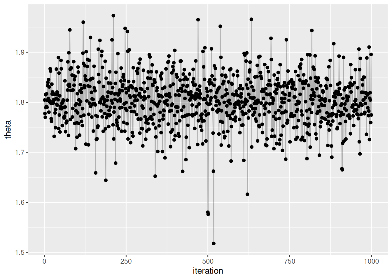
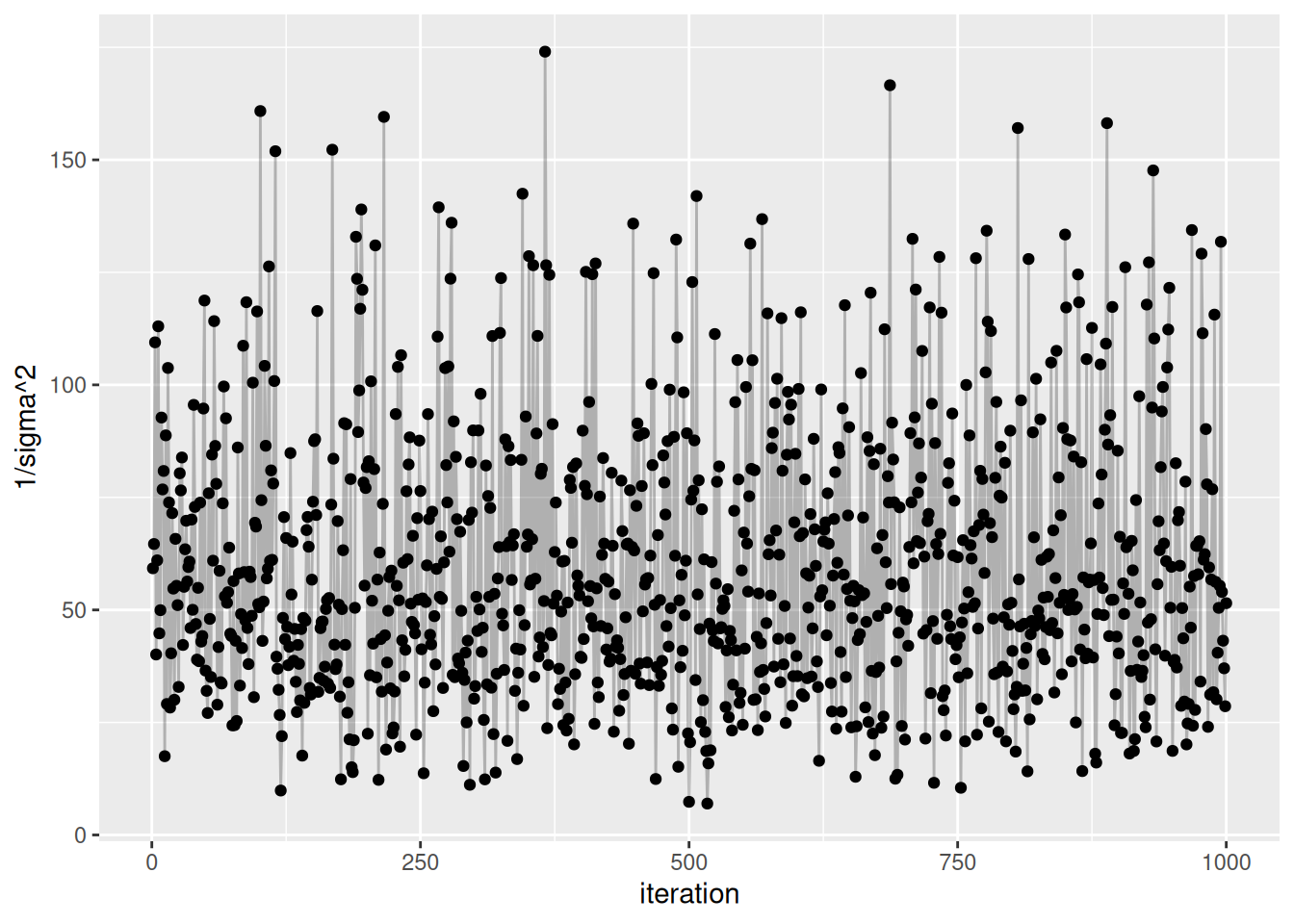
Back to midge length. Here are the traceplots for our samples of theta and sigma^2:

midge.df$iteration = midge.df$n
ggplot(midge.df, aes(x = iteration, y = theta)) +
  geom_point() + geom_line(alpha = 0.25)

ggplot(midge.df, aes(x = iteration, y = `1/sigma^2`)) +
  geom_point() + geom_line(alpha = 0.25)

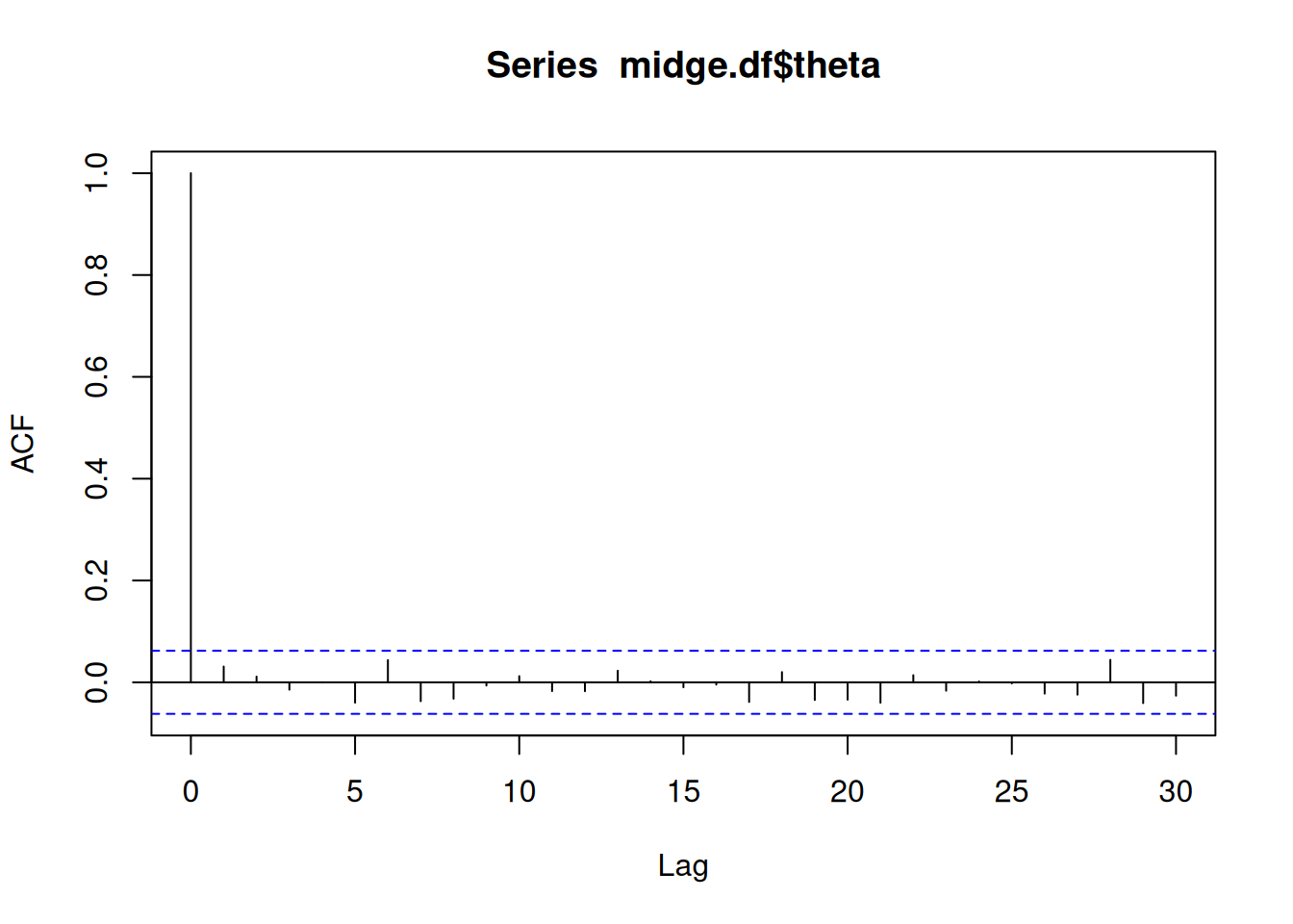
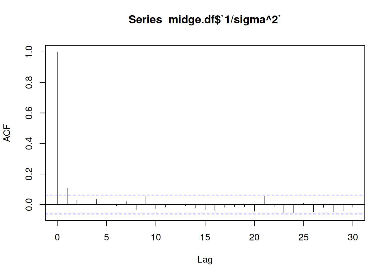
By viewing the autocorrelation function and effective sample sizes of our data, we can see that the samples look quite good and seem to have reasonable effective sample sizes.

acf(midge.df$theta)

effectiveSize(midge.df$theta)
#> var1 
#> 1000
acf(midge.df$`1/sigma^2`)

effectiveSize(midge.df$`1/sigma^2`)
#>     var1 
#> 805.4388

7 Exercises

7.1 6.1

a

\[ \begin{aligned} \text{Cov}(\theta_A, \theta_B) &= \mathbb{E}\left[\theta_A \theta_B\right] - \mathbb{E}[\theta_A]\mathbb{E}[\theta_B] \\ &= \mathbb{E}[\theta^2\gamma] - \mathbb{E}[\theta] \mathbb{E}[\theta\gamma] \\ &= \mathbb{E}\left[\theta^2\right] \mathbb{E}\left[ \gamma \right] - \mathbb{E}[\theta]\mathbb{E}[\theta]\mathbb{E}[\gamma] & \theta \perp \gamma \\ &= \mathbb{E}\left[\theta^2\right] \mathbb{E}\left[ \gamma \right] - \mathbb{E}[\theta]^2\mathbb{E}[\gamma] \\ &= \left(\mathbb{E}[\theta^2] - \mathbb{E}[\theta]^2 \right) \mathbb{E}[\gamma] \\ &= \text{Var}(\theta) \mathbb{E}[\gamma] \\ &\neq 0 \end{aligned} \]

Since \(\text{Cov}(\theta_A, \theta_B) \neq 0\), \(\theta_A\) and \(\theta_B\) are dependent.

This prior is justified if we have reason to believe that \(\theta_B\) is some product of \(\theta_A\) plus random Gamma-distributed noise.

b

First the joint posterior distribution

\[ \begin{aligned} p(\theta, \gamma \mid \boldsymbol{y}_A, \boldsymbol{y}_B) &\propto p(\theta, \gamma) \times p(\boldsymbol{y}_A, \boldsymbol{y}_B \mid \theta, \gamma) \\ &= p(\theta) \times p(\gamma) \times p(\boldsymbol{y}_A \mid \theta) \times p(\boldsymbol{y}_B \mid \theta, \gamma) & \boldsymbol{y}_A \perp \gamma \\ &\propto \left(\theta^{a_\theta - 1}e^{-b_\theta \theta}\right) \times \left(\gamma^{a_\gamma - 1}e^{-b_\gamma \gamma} \right) \times \left(\prod_{i=1}^{n_{A}} \theta^{y_{A_i}} e^{-\theta} \right) \times \left(\prod_{i=1}^{n_{B}} (\gamma \theta)^{y_{B_i}} e^{-\gamma \theta} \right) \\ &= \left(\theta^{a_\theta - 1}e^{-b_\theta \theta}\right) \times \left(\gamma^{a_\gamma - 1}e^{-b_\gamma \gamma} \right) \times \left( \theta^{\sum_{i = 1}^{n_A} y_{A_i}} e^{-n_A \theta} \right) \times \left( (\gamma \theta)^{\sum_{i=1}^{n_B} y_{B_i}} e^{- n_B \gamma \theta} \right) \\ &= \left(\theta^{a_\theta - 1}e^{-b_\theta \theta}\right) \times \left(\gamma^{a_\gamma - 1}e^{-b_\gamma \gamma} \right) \times \left( \theta^{n_A \bar{y}_A} e^{-n_A \theta} \right) \times \left( (\gamma \theta)^{n_B \bar{y}_B} e^{- n_B \gamma \theta} \right) \\ \end{aligned} \]

So

\[ \begin{aligned} p(\theta, \mid \boldsymbol{y}_A, \boldsymbol{y}_B, \gamma) &\propto \left(\theta^{a_\theta - 1}e^{-b_\theta \theta}\right) \times \left(\gamma^{a_\gamma - 1}e^{-b_\gamma \gamma} \right) \times \left( \theta^{n_A \bar{y}_A} e^{-n_A \theta} \right) \times \left( (\gamma \theta)^{n_B \bar{y}_B} e^{- n_B \gamma \theta} \right) \\ &\propto \left(\theta^{a_\theta - 1}e^{-b_\theta \theta}\right) \times \left( \theta^{n_A \bar{y}_A} e^{-n_A \theta} \right) \times \left( (\gamma \theta)^{n_B \bar{y}_B} e^{- n_B \gamma \theta} \right) \\ &\propto \theta^{a_\theta + n_A \bar{y}_A + n_B \bar{y}_B - 1} \exp \left( - (b_\theta + n_A + n_B \gamma ) \theta \right) \\ &\propto \text{dgamma}\left(a_\theta + n_A \bar{y}_A + n_B \bar{y}_B, b_\theta + n_A + n_B \gamma \right) \end{aligned} \]

c

\[ \begin{aligned} p(\gamma, \mid \boldsymbol{y}_A, \boldsymbol{y}_B, \theta) &\propto \left(\theta^{a_\theta - 1}e^{-b_\theta \theta}\right) \times \left(\gamma^{a_\gamma - 1}e^{-b_\gamma \gamma} \right) \times \left( \theta^{n_A \bar{y}_A} e^{-n_A \theta} \right) \times \left( (\gamma \theta)^{n_B \bar{y}_B} e^{- n_B \gamma \theta} \right) \\ &\propto \left(\gamma^{a_\gamma - 1}e^{-b_\gamma \gamma} \right) \times \left( (\gamma \theta)^{n_B \bar{y}_B} e^{- n_B \gamma \theta} \right) \\ &\propto \left(\gamma^{a_\gamma - 1}e^{-b_\gamma \gamma} \right) \times \left( \gamma^{n_B \bar{y}_B} e^{- n_B \gamma \theta} \right) \\ &\propto \gamma^{a_\gamma + n_B \bar{y}_B - 1} \exp\left( -(b_\gamma + n_B \theta) \gamma \right) \\ &\propto \text{dgamma}\left(a_\gamma + n_B\bar{y}_B, b_\gamma + n_B \theta \right) \end{aligned} \]

d

Y_a <- scan('Exercises/menchild30bach.dat')
Y_b <- scan('Exercises/menchild30nobach.dat')
n_a = length(Y_a)
n_b = length(Y_b)
ybar_a = mean(Y_a)
ybar_b = mean(Y_b)

a_theta = 2
b_theta = 1

S = 5000

ab_gamma = c(8, 16, 32, 64, 128)

theta_diff = sapply(ab_gamma, function(abg) {
  a_gamma = b_gamma = abg

  THETA = numeric(S)
  GAMMA = numeric(S)

  # Starting values
  theta = ybar_a
  gamma = ybar_a / ybar_b  # Relative rate \theta_B / \theta_A

  for (s in 1:S) {
    # Sample theta \text{dgamma}\left(a_\theta + n_A \bar{y}_A + n_B \bar{y}_B, b_\theta + n_A + n_B \gamma \right)
    theta = rgamma(
      1,
      a_theta + n_a * ybar_a + n_b * ybar_b,
      b_theta + n_a + n_b * gamma
    )

    # Sample gamma from \text{dgamma}\left(a_\gamma + n_B\bar{y}_B, b_\gamma + n_B \theta \right)
    gamma = rgamma(
      1,
      a_gamma + n_b * ybar_b,
      b_gamma + n_b * theta
    )

    THETA[s] = theta
    GAMMA[s] = gamma
  }

  # Reconstruct \theta_A, \theta_B
  THETA_A = THETA
  THETA_B = THETA * GAMMA

  mean(THETA_B - THETA_A)
})

ggplot(data.frame(ab_gamma = ab_gamma, theta_diff = theta_diff), aes(x = ab_gamma, y = theta_diff)) +
  geom_point() +
  geom_line()

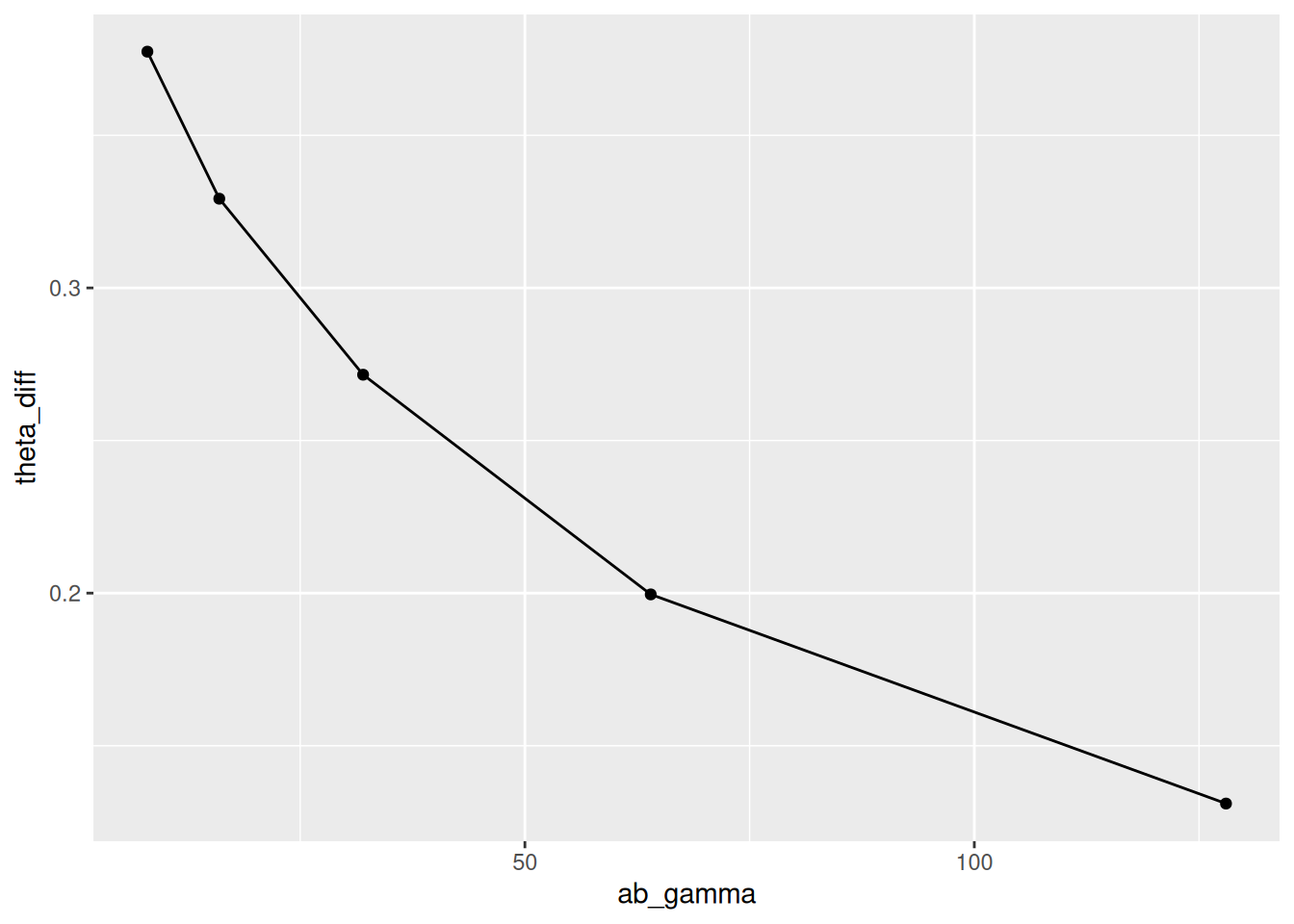
Since \(a_\gamma\) and \(b_\gamma\) are equal, the gamma distribution is centered around 1 and the magnitude represents the strength of our belief that \(\gamma\) (the proportion \(\theta_B / \theta_A\)) is 1. As expected, as our belief in that increases, the mean posterior difference between \(\theta_B\) and \(\theta_A\) decreases.

7.2 6.2

glucose <- scan('Exercises/glucose.dat')

a

qplot(glucose, geom = 'histogram')

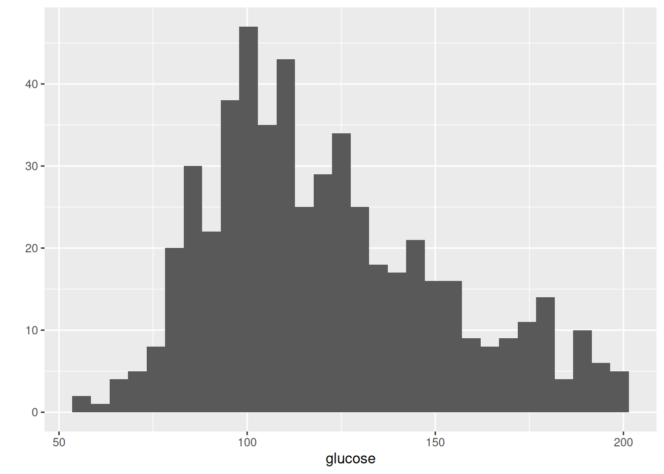
Appears to be skewed right significantly.

b

The likelihood is

\[ \begin{aligned} p(\boldsymbol{y} \mid \boldsymbol{x}, p, \theta_1, \theta_2, \sigma^2_1, \sigma^2_2) &= \prod_{i = 1}^n p(y_i \mid x_i, p, \theta_1, \theta_2, \sigma^2_1, \sigma^2_2) \\ &= \prod_{i = 1}^n \text{dnorm}(y_i, \theta_1, \sigma^2_1)^{x_i} \text{dnorm}(y_i, \theta_2, \sigma^2_2)^{1 - x_i} \\ \end{aligned} \]

\(\boldsymbol{x}\)

First observe the probability that a single \(X_i = 1\):

\[ \begin{aligned} P(X_i = 1 \mid y_i, p, \theta_1, \theta_2, \sigma^2_1, \sigma^2_2) &= \frac{P(X_i = 1 \mid p, \theta_1, \theta_2, \sigma^2_1, \sigma^2_2) \times p(y_i \mid X_i = 1, p, \theta_1, \theta_2, \sigma^2_1, \sigma^2_2)}{P(y_i \mid p, \theta_1, \theta_2, \sigma^2_1, \sigma^2_2)} \\ &= \frac{P(X_i = 1 \mid p) \times p(y_i \mid X_i = 1, \theta_1, \sigma^2_1)}{P(X_i = 1 \mid p) \times p(y_i \mid X_i = 1, \theta_1, \sigma^2_1) + P(X_i = 0 \mid p) \times p(y_i \mid X_i = 0, \theta_2, \sigma^2_2)} \\ &= \frac{p \times \text{dnorm}(y_i, \theta_1, \sigma^2_1)}{p \times \text{dnorm}(y_i, \theta_1, \sigma^2_1) + (1 - p) \times \text{dnorm}(y_i, \theta_2, \sigma^2_2)} \end{aligned} \]

Since this is similar for \(P(X_i = 0)\), we know

\[ x_i \sim \text{Bernoulli}\left(\frac{p \times \text{dnorm}(y_i, \theta_1, \sigma^2_1)}{p \times \text{dnorm}(y_i, \theta_1, \sigma^2_1) + (1 - p) \times \text{dnorm}(y_i, \theta_2, \sigma^2_2)}\right) \]

\(p\)

For this and later calculations, let \(n_1 = \sum x_i\) (i.e. number of 1s in \(\boldsymbol{x}\)) and \(n_2 = n - n_1\) (i.e. number of 0s).

\[ \begin{aligned} p(p \mid \boldsymbol{x}, \boldsymbol{y}, \theta_1, \theta_2, \sigma^2_1, \sigma^2_2) &\propto p(p) \times p(\boldsymbol{x}, \boldsymbol{y}, \theta_1, \theta_2, \sigma^2_1, \sigma^2_2 \mid p) \\ &\propto p(p) \times p(\boldsymbol{x} \mid p) p(\boldsymbol{y} \mid \boldsymbol{x}, \theta_1, \theta_2, \sigma^2_1, \sigma^2_2) p(\theta_1, \theta_2, \sigma^2_1, \sigma^2_2) \\ &\propto p(p) \times p(\boldsymbol{x} \mid p) \\ &\propto \text{dbeta}(p, a, b) \times \text{dbinom}(n_1, n, p) \\ &\propto p^{a - 1} (1 - p)^{b - 1} \times p^{n_1} (1 - p)^{n_2} \\ &= p^{a + n_1 - 1}(1 - p)^{b + n_2 - 1} \\ &= \text{dbeta}(p, a + n_1, b + n_2) \end{aligned} \]

\(\theta_1\)

Let \(\boldsymbol{y}_1 = \{y_i \in \boldsymbol{y} \; : \; x_i = 1 \}\) and \(\boldsymbol{y}_2 = \{y_i \in \boldsymbol{y} \; : \; x_i = 0 \}\)

\[ \begin{aligned} p(\theta_1 \mid \boldsymbol{x}, \boldsymbol{y}, p, \theta_2, \sigma^2_1, \sigma^2_2) &\propto p(\theta_1 \mid \boldsymbol{x}, p, \theta_2, \sigma^2_1, \sigma^2_2) \times p(\boldsymbol{y} \mid \boldsymbol{x}, p, \theta_1, \theta_2, \sigma^2_1, \sigma^2_2) \\ &\propto p(\theta_1) \times \prod_{i=1}^n \left( \text{dnorm}(y_i, \theta_1, \sigma^2_1)^{x_i} \text{dnorm}(y_i, \theta_2, \sigma^2_2)^{1 - x_i} \right) \\ &\propto \text{dnorm}(\theta_1, \mu_0, \tau^2_0) \times \prod_{i = 1}^n \text{dnorm}(y_i, \theta_1, \sigma^2_1)^{x_i} \\ &\propto \text{dnorm}(\theta_1, \mu_0, \tau^2_0) \times \prod_{y \in \boldsymbol{y}_1} \text{dnorm}(y, \theta_1, \sigma^2_1) \\ &\propto \exp \left(- \frac{1}{2 \tau^2_0} (\theta_1 - \mu_0)^2 \right) \times \prod_{y \in \boldsymbol{y}_1} \exp\left( -\frac{1}{2\sigma^2_1} (y - \theta_1)^2\right) \\ &\propto \exp \left(- \frac{1}{2 \tau^2_0} (\theta_1 - \mu_0)^2 \right) \times \exp\left(-\frac{1}{2\sigma^2_1} \sum_{y \in \boldsymbol{y}_1} (y - \theta_1)^2 \right) \\ &\propto \text{calculations from 5.2...} \\ &\propto \mathcal{N}(\tau^2_{n , 1}, \mu_{n, 1}) \end{aligned} \]

where

\[ \begin{aligned} \tau^2_{n, 1} &= \frac{1}{\frac{1}{\tau^2_0} + \frac{n_1}{\sigma^2_1}} \\ \mu_{n, 1} &= \frac{\frac{1}{\tau^2_0}\mu_0 + \frac{n_1}{\sigma^2_1} \bar{y}_{\cdot, 1}}{\frac{1}{\tau^2_0} + \frac{n_1}{\sigma^2_1}} \end{aligned} \]

\(\theta_2\)

\(\theta_2 \mid \dots \sim \mathcal{N}(\mu_{n, 2}, \tau^2_{n, 2})\) like \(\theta_1\) but with the subscripts switched from 1 to 2.

\(\sigma^2_1\)

As probably expected, this will look like inference for a standard normal model, except using only the data in group 1.

\[ \begin{aligned} p(\sigma^2_1 \mid \boldsymbol{x}, \boldsymbol{y}, p, \theta_1, \theta_2, \sigma^2_2) &\propto p(\sigma^2_1 \mid \boldsymbol{x}, p, \theta_1, \theta_2, \sigma^2_2) \times p(\boldsymbol{y} \mid \boldsymbol{x}, p, \theta_1, \theta_2, \sigma^2_1, \sigma^2_2) \\ &\propto p(\sigma^2_1) \times \prod_{i=1}^n \left( \text{dnorm}(y_i, \theta_1, \sigma^2_1)^{x_i} \text{dnorm}(y_i, \theta_2, \sigma^2_2)^{1 - x_i} \right) \\ &\propto \text{inverse-gamma}(\sigma^2_1, \nu_0, \sigma^2_0 \nu_0 / 2) \times \prod_{y \in \boldsymbol{y}_1} \text{dnorm}(y, \theta_1, \sigma^2_1) \\ &\propto \exp \left((\sigma_1^2)^{-(\nu_0 / 2) - 1} \exp\left( -\frac{1}{\sigma^2_1} \sigma^2_0 \nu_0 / 2 \right) \right) \times (\sigma_1^2)^{-n / 2} \exp\left(-\frac{1}{2\sigma^2_1} \sum_{y \in \boldsymbol{y}_1} (y - \theta_1)^2 \right) \\ &\propto \text{calculations from 6.3...} \\ &\propto \text{inverse-gamma}(\nu_{n, 1} / 2, \sigma^2_{n, 1}(\theta_1) \nu_{n, 1} / 2) \end{aligned} \]

where

\[ \begin{aligned} \nu_{n, 1} &= \nu_0 + n_1 \\ \sigma^2_{n, 1}(\theta_1) &= \frac{1}{\nu_{n, 1}} \left[\nu_0 \sigma^2_0 + n_1 s^2_{n, 1}(\theta_1) \right] \end{aligned} \]

\(\sigma^2_2\)

Same as above, but with subscripts switched.

c

Y = glucose
n = length(Y)

# Priors
a = b = 1
mu0 = 120
t20 = 200
s20 = 1000
nu0 = 10

S = 10000

# Values we'd like to store. Don't care about xs, p, sigmas
THETA1 = numeric(S)
THETA2 = numeric(S)
YPRED = numeric(S) # Posterior predictive

# Starting values
p = 0.5
theta1 = theta2 = mean(Y)
s21 = s22 = var(Y)

# Gibbs sampling
for (s in 1:S) {
  # Sample X
  # We calculate dnorm for each y so p1 and p2 are vectors
  p1 = p * dnorm(Y, theta1, sqrt(s21))
  p2 = (1 - p) * dnorm(Y, theta2, sqrt(s22))
  bernoulli_p = p1 / (p1 + p2)
  X = rbinom(n, 1, bernoulli_p)
  
  # With X sample, calcuate group-specific summary statistics
  n1 = sum(X)
  n2 = n - n1
  y1 = Y[X == 1]
  y2 = Y[X == 0]
  ybar1 = mean(y1)
  ybar2 = mean(y2)
  yvar1 = var(y1)
  yvar2 = var(y2)
  
  # Sample p
  p = rbeta(1, a + n1, b + n2)
  
  # Sample thetas
  t2n1 = 1 / (1 / t20 + n1 / s21)
  mun1 = (mu0 / t20 + n1 * ybar1 / s21) / (1 / t20 + n1 / s21)
  theta1 = rnorm(1, mun1, sqrt(t2n1))
  
  t2n2 = 1 / (1 / t20 + n2 / s22)
  mun2 = (mu0 / t20 + n2 * ybar2 / s22) / (1 / t20 + n2 / s22)
  theta2 = rnorm(1, mun2, sqrt(t2n2))

  # Sample sigma^2s
  nun1 = nu0 + n1
  s2n1 = (nu0 * s20 + (n1 - 1) * yvar1 + n1 * (ybar1 - theta1)^2) / nun1
  s21 = 1 / rgamma(1, nun1 / 2, s2n1 * nun1 / 2)

  nun2 = nu0 + n2
  s2n2 = (nu0 * s20 + (n2 - 1) * yvar2 + n2 * (ybar2 - theta2)^2) / nun2
  s22 = 1 / rgamma(1, nun2 / 2, s2n2 * nun2 / 2)
  
  # Sample posterior predictive
  xpred = runif(1) < p
  ypred = ifelse(xpred, rnorm(1, theta1, sqrt(s21)), rnorm(1, theta2, sqrt(s22)))
  
  # Store values
  THETA1[s] = theta1
  THETA2[s] = theta2
  YPRED[s] = ypred
}

THETAMIN = pmin(THETA1, THETA2)
THETAMAX = pmax(THETA1, THETA2)

library(coda)

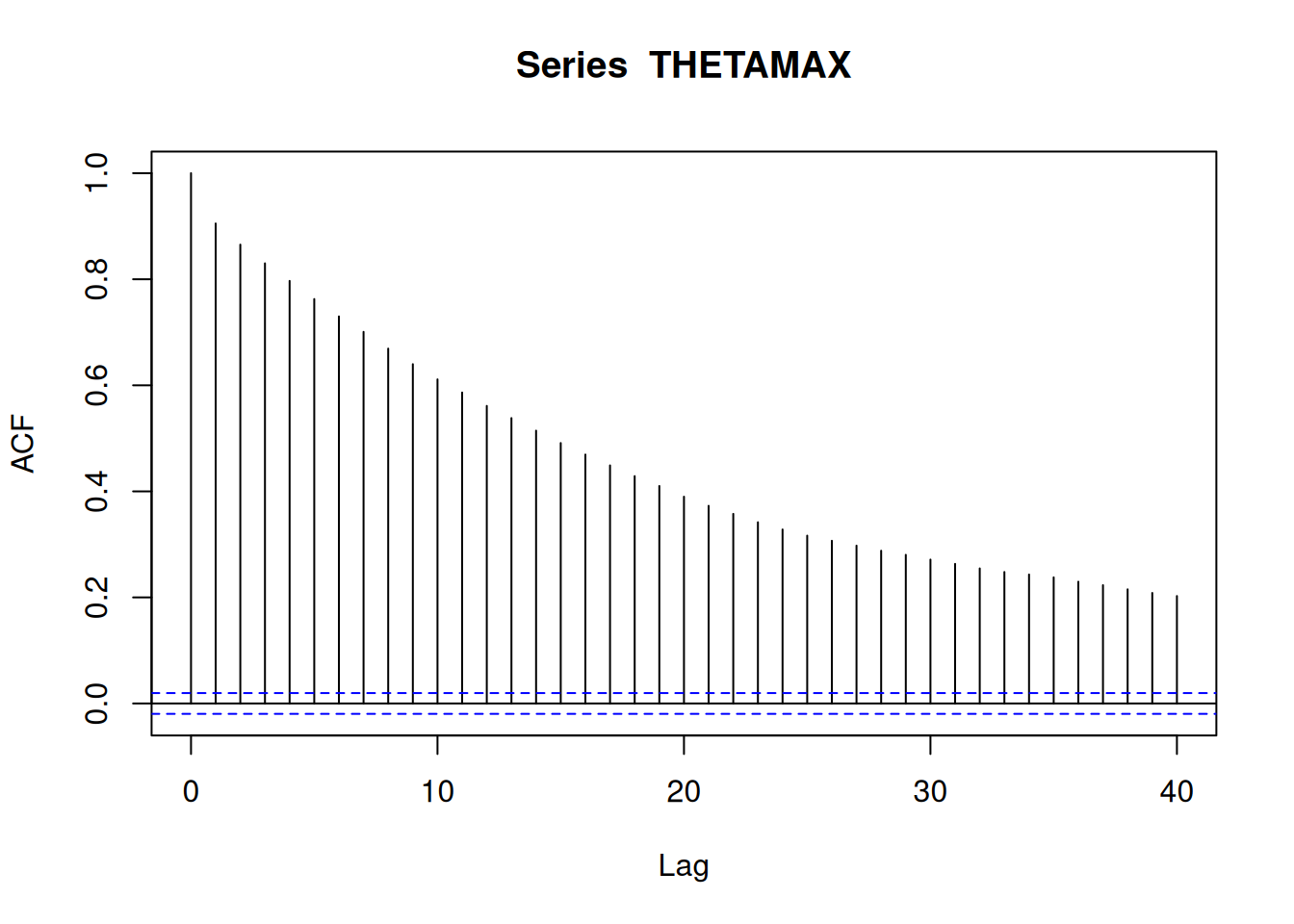
acf(THETAMIN)

effectiveSize(THETAMIN)
#>     var1 
#> 534.7286

acf(THETAMAX)

effectiveSize(THETAMAX)
#>     var1 
#> 227.5474

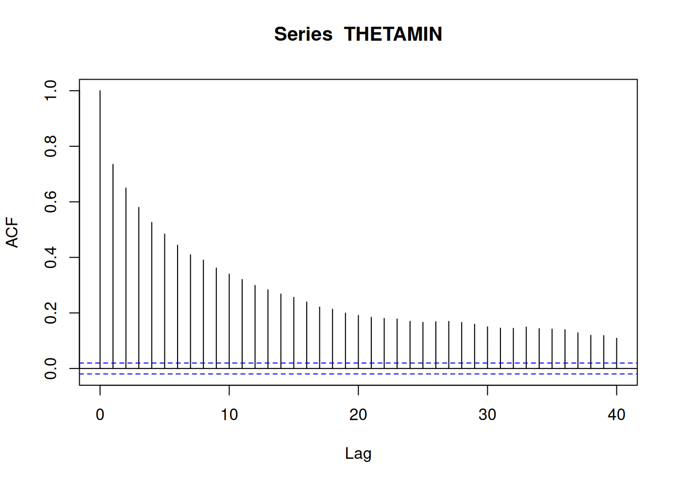
These samples are actually highly autocorrelated, hence the minimum effective sample sizes. However, the purpose of calculating the autocorrelation of the minimum and maximum \(\theta\) is unclear.

d

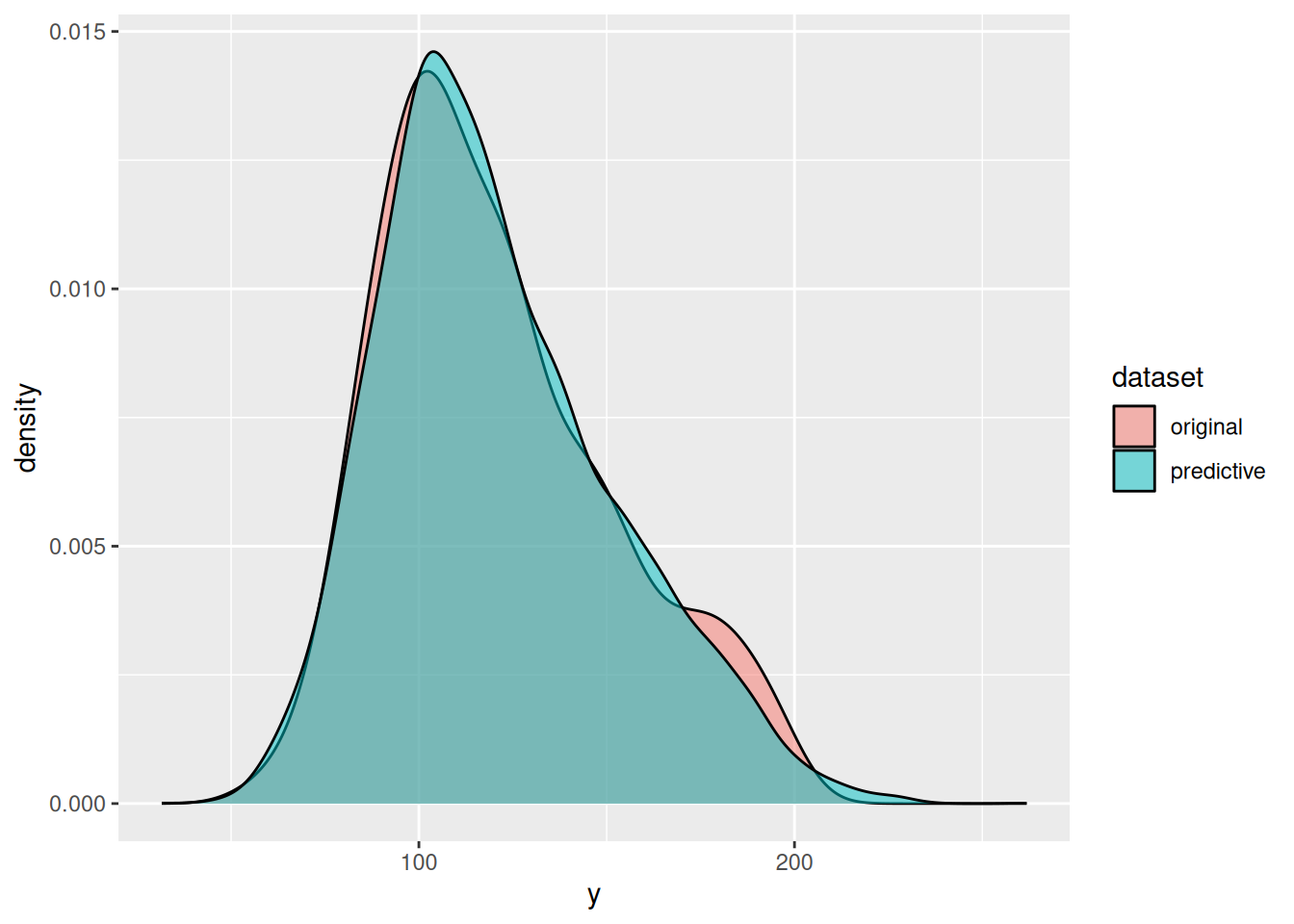
YCOMP = rbind(data.frame(y = YPRED, dataset = 'predictive'), data.frame(y = Y, dataset = 'original'))
ggplot(YCOMP, aes(x = y, fill = dataset)) +
  geom_density(alpha = 0.5)

Based on the very close correspondence with the densities of the original and posterior predictive dataset, it seems like this mixture model fits very well.

Marmer, Vadim. 2010. “The Gibbs Sampler.” http://faculty.arts.ubc.ca/vmarmer/econ627/627_10_02.pdf.