Chapter 1: Introduction and examples

Jesse Mu

2016-09-07

1 Introduction

Bayesian inference: the process of learning by updating prior probabilistic beliefs in light of new information. Data analysis tools built on these foundations are known as Bayesian methods.

1.1 The Bayesian learning framework

We want to estimate a parameter \(\theta \in \Theta\) from a dataset \(y \in \mathcal{Y}\).

• \(p(\theta)\), defined for all \(\theta \in \Theta\), is our prior distribution about the space of possible parameters
• Bayesian methods require a sampling model: \(P(y \mid \theta)\) describes the probability that of a specific dataset given a parameter.
  • Note that later, this will be useful for prediction!

Then we wish to update our belief distribution about \(\theta\) given. The posterior distribution is defined as

\[\begin{align} p(\theta \mid y) = \frac{p(y \mid \theta) p(\theta)}{\int_{\Theta}p(y \mid \tilde{\theta}) p(\tilde{\theta}) \; d\tilde{\theta}}. \end{align}\]

Note that the denominator is constant and doesn’t need to be computed, since we can just normalize our posterior distribution such that \(P(\theta \mid y)\) for all \(\Theta\) sums up to 1. Thus we commonly write

\[\begin{align} p(\theta \mid y) \propto p(y \mid \theta) p(\theta). \end{align}\]

versus frequentist learning

(from Resnik and Hardisty 2010)

The difference between Bayesian learning and frequentist learning is the consideration of prior beliefs about parameters. In standard Maximum Likelihood Estimation (MLE), we select the parameter that is most likely to have generated the observed data:

\[ \theta_{ML} = \underset{\theta}{\text{argmax}} \; p(y \mid \theta). \]

Using Bayesian Maximum A Posteriori Estimation, however, we select \(\theta\) that is most likely given the observed data. The difference is that our measure of “likelihood given the data” is influenced by our prior beliefs about \(\theta\), as in Equation 2:

\[\begin{align} \theta_{MAP} &= \underset{\theta}{\text{argmax}} \; p(\theta \mid y) \\ &= \underset{\theta}{\text{argmax}} p(y \mid \theta) p(\theta). \end{align}\]

Note that with an uninformative prior \(\theta \sim \text{Uniform}\), the MAP estimate is the same as the ML estimate.

2 Why Bayes?

2.1 As an approach to probability and statistics

The debate between Bayesians and frequentists dives into some very philosophical issues. Cox’s theorem (1946, 1961) gives a formal proof for thinking about probabilities using a Bayesian approach. An explanation of these proofs can be found in Van Horn (2003).

Outside of formal mathematical grounding, Bayesian methods have excellent practical benefits as data analysis tools:

1. Even if prior probabilities are not exactly quantifiable, approximations of \(p(\theta)\) and \(p(\theta \mid y)\) are still useful for analyzing how rational learners would change beliefs
2. Bayesian methods can represent principled ways of doing analysis when there are no alternative methods

2.2 As models of cognition

An appeal of Bayesian learning is that it is also cognitively intuitive. Humans have beliefs about the world, whose uncertainty can be expressed probabilistically. Then, given data, these beliefs are rationally updated.

There is a rich tradition in modeling human cognition using Bayesian methods to great success, with plenty of work done in showing how people’s beliefs and knowledge about the world can be expressed probabilistically (e.g., Griffiths and Tenenbaum 2006)

Bayesianism is not without its detractors, however. Some critics argue that the evidence that Bayesian analysis is weak, and that sufficiently sophisticated models are unfalsifiable. See Bowers and Davis (2012a), comment by Griffiths et al. (2012), reply by Bowers and Davis (2012b).

3 Example 1: Estimating the probability of a rare event

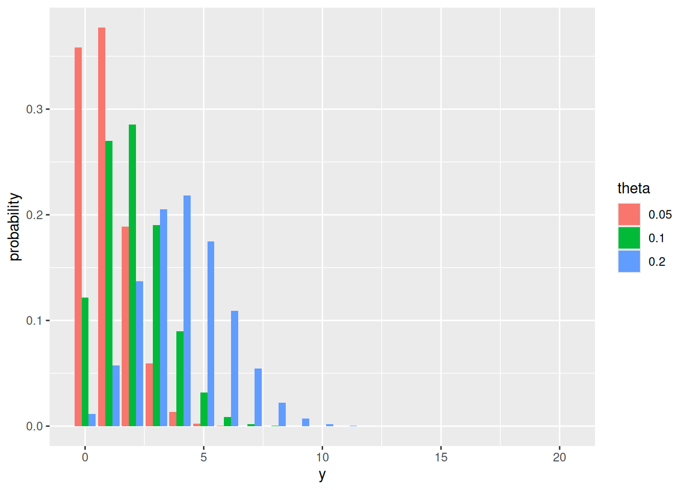
We are interested in the prevelance of a disease in a city. Let \(\theta \in [0, 1]\) be the fraction of infected individuals. We take a sample of 20 individuals and record the number of individuals \(y \in Y = {0, 1, \dots, 20}\) with the disease.

The sampling model is

\[ Y \mid \theta \sim \text{Binomial}(20, \theta), \]

i.e. each individual has an independent \(\theta\)% chance of having the disease.

d = data.frame(
  y = 0:20,
  theta = factor(rep(c(0.05, 0.10, 0.20), each = 21)),
  probability = c(dbinom(0:20, 20, 0.05), dbinom(0:20, 20, 0.1), dbinom(0:20, 20, 0.2))
)
ggplot(d, aes(x = y, y = probability, fill = theta)) +
  geom_bar(stat = "identity", position = "dodge")

For various theta, the probability of observing y infected individuals in the sample.

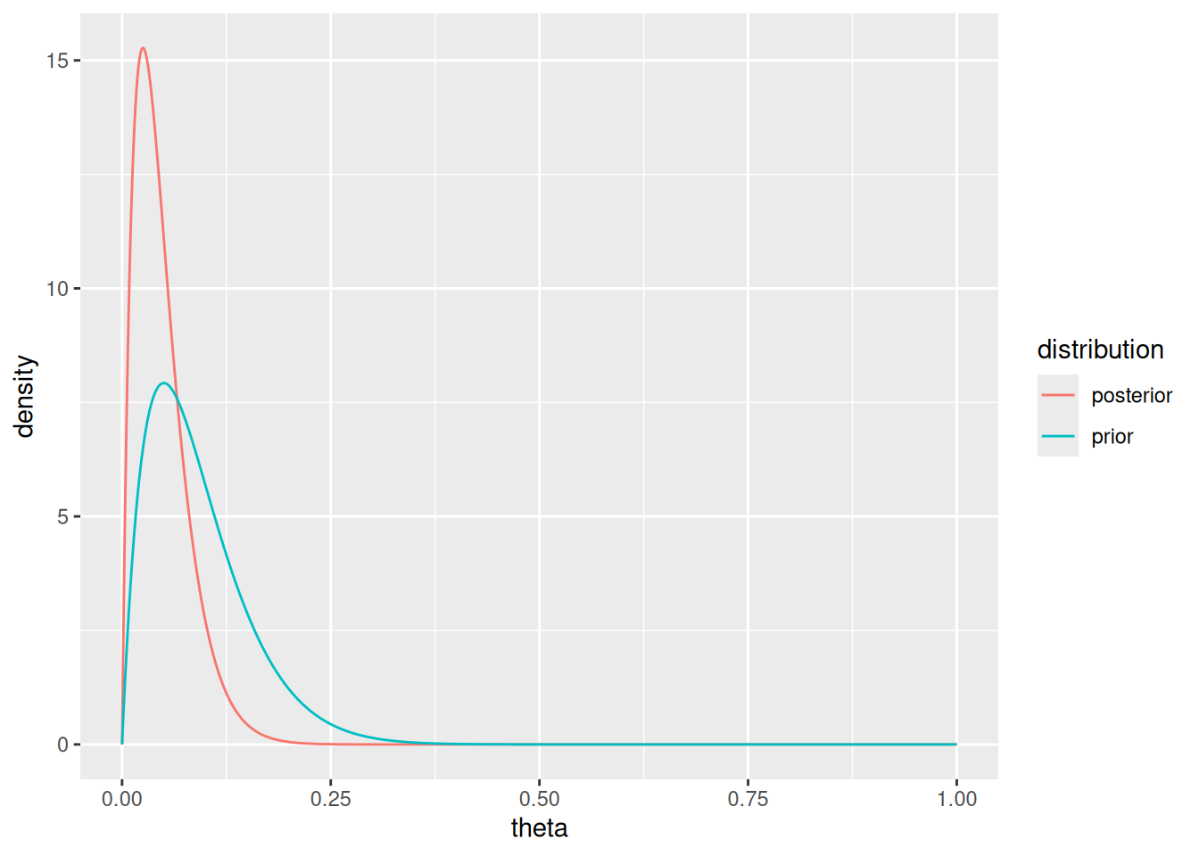
Imagine we believe \(\theta\) is probably in the interval \([0.05, 0.20]\). For computational convenience, we will encode this prior as a Beta distribution

\[ \theta \sim \text{Beta}(2, 20) \]

Conveniently, (we will prove this later), given \(Y \mid \theta \sim \text{Binomial}(n, \theta)\) and \(\theta \sim \text{Beta}(a, b)\),

\[ (\theta \mid Y = y) \sim \text{Beta}(a + y, b + n - y). \]

For example, if we observe 0/20 individuals infected, \(\theta \mid {Y = 0} \sim \text{Beta}(2, 40)\).

d = data.frame(
  theta = seq(0, 1, by = 0.001),
  distribution = rep(c("prior", "posterior"), each = 1001),
  density = c(dbeta(seq(0, 1, by = 0.001), 2, 20), dbeta(seq(0, 1, by = 0.001), 2, 40))
)
ggplot(d, aes(x = theta, y = density, color = distribution)) +
  geom_line()

Prior and posterior distributions on theta after observing 0/20 infected individuals. Note the posterior is more tightly peaked around near-zero values.

Notice that Bayesian and frequentist approaches to parameter estimation differ:

\[\begin{align} \theta_{ML} &= \underset{\theta}{\text{argmax}} \; P(Y = 0 \mid \theta) = 0 \\ \theta_{MAP} &= \underset{\theta}{\text{argmax}} \; P(\theta \mid Y = 0) = \text{Mode}(\theta \mid Y = 0) = 0.025 \end{align}\]

but also notice that the point estimate is NOT equal to the expectation of \(\theta\), since \(\mathbb{E}(\theta \mid Y = 0) = 0.048\). We will probably later determine when to use the expectation over the mode.

Finally, notice that we can do very intuitive statistical tests (e.g \(P(\theta < 0.10 \mid Y = 0)\)) by measuring the areas under our posterior distribution.

3.1 Sensitivity analysis

If we change the confidence in our prior, we get different posterior distributions. The more “peaked” our prior is, the less peaked the posterior will be given a \(Y = 0\) result (and the less the Bayesian solution will approximate the ML estimate).

To quantify how changes in the prior beliefs affect our posterior estimates, we’ll do some calculations. Recall the expectation and variance of Beta distributions. If \(X \sim \text{Beta}(\alpha, \beta)\), then

\[\begin{align} \mathbb{E}(X) &= \frac{\alpha}{\alpha + \beta} \\ \text{Var}(X) &= \frac{\alpha \beta}{(\alpha + \beta)^2 (\alpha + \beta + 1)}. \end{align}\]

Due to the properties of these functions we can parameterize the Beta distribution alternatively with

• Expectation: \(\theta_0 = \frac{\alpha}{\alpha + \beta}\)
• Precision: \(w = a + b\)

Since \((\theta \mid Y = y) \sim \text{Beta}(a + y, b + n - y)\),

\[\begin{align} \mathbb{E}(\theta \mid Y = y) &= \frac{a + y}{a + b + n} \\ &= \frac{n}{w + n}\frac{y}{n} + \frac{w}{w + n}\theta_0. \end{align}\]

# What is the expected value of theta after observing result y, given a Beta
# prior parameterized by theta0 and w?
N = 20
exp.posterior = function(w, theta0, y) {
  (N / (w + N)) * (y / N) + (w / (w + N)) * theta0
}
Theta0 = rev(seq(0.0, 0.5, by = 0.01))
W = seq(0, 25, by = 0.5)
d = outer(Theta0, W, FUN = function(w, theta0) exp.posterior(w, theta0, 0))
rownames(d) = Theta0
colnames(d) = W

df = as.data.frame(d) |>
  tibble::rownames_to_column('theta0') |>
  pivot_longer(cols = -theta0, names_to = 'w', values_to = 'theta') |>
  mutate(theta0 = as.numeric(theta0), w = as.numeric(w))

p = ggplot(df, aes(x = w, y = theta0, z = theta)) +
  geom_contour(aes(colour = ..level..))
library(directlabels)
direct.label(p, method = 'bottom.pieces')

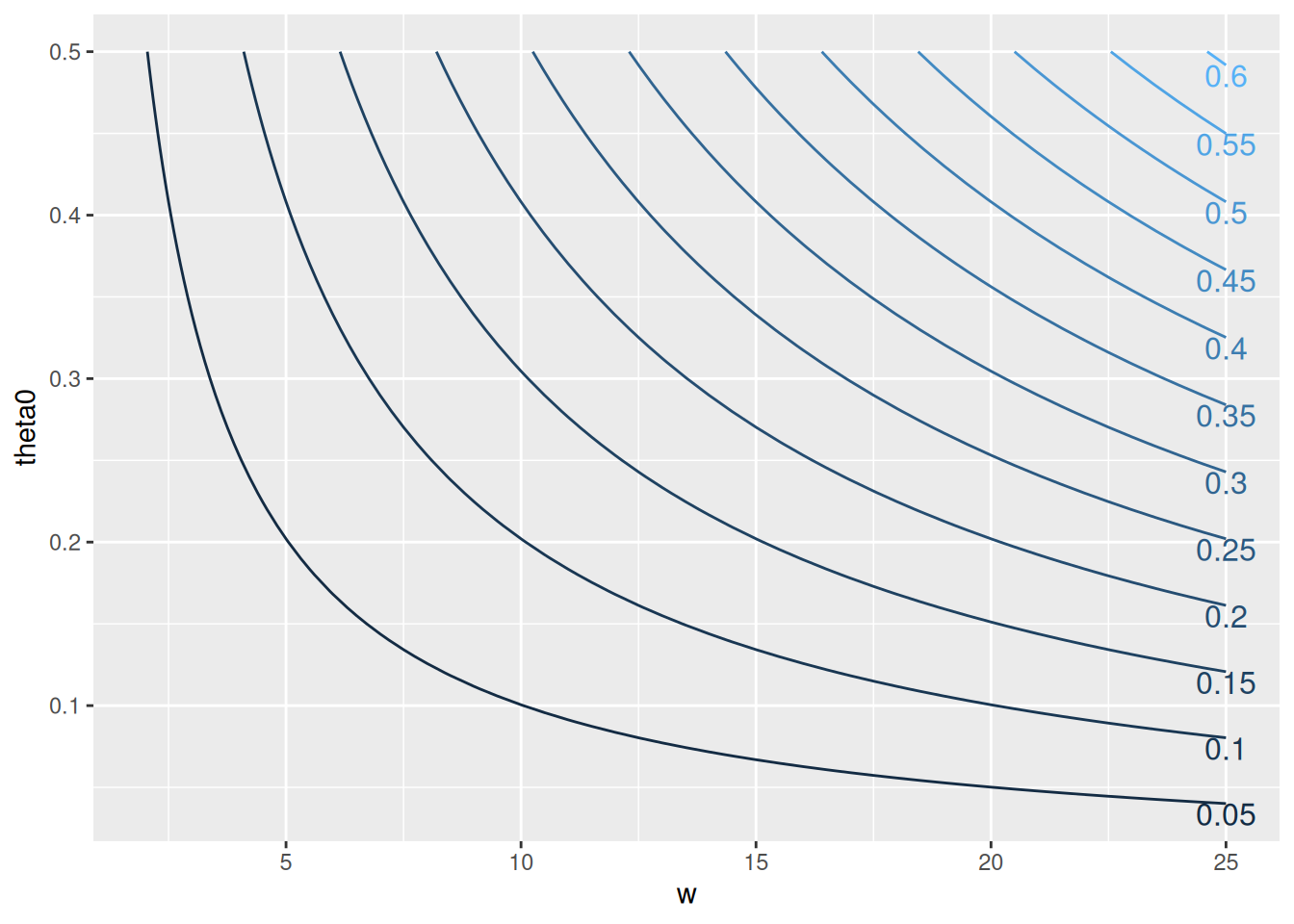
Expected value of the posterior for theta, for combinations of theta0 and w

3.2 Comparison to non-Bayesian methods

When we use the frequentist maximum likelihood estimator, we get an estimated \(\theta_{ML} = 0\). Since our estimate is subject to sampling error, we commonly construct confidence intervals for these estimates.

The Wald interval is a commonly used confidene interval for a population proportion. However, it is not meant to be used for small sample sizes or situations in which the observed proportion is close to (or equals) 0 or 1, since in these cases the error of a binomially-distributed observation is not at all like the normal distribution For an observation \(Y = 20\), for example, the Wald CI is, regardless of level of confidence, just \(0\). We wouldn’t want to say with 99.999% confidence that the population mean is 0, given our small sample size.

The previous Bayesian estimate, however, works well for both small and large n.  With small \(n\), the estimator allows us to encode prior beliefs about the true proportion. With \(w\) and \(\theta_0\) as before:

\[ \hat{\theta} = \mathbb{E}(\theta \mid Y = y) = \frac{n}{n + w}\frac{y}{n} + \frac{w}{n + w}\theta_0. \]

Notice that this is kind of an average between the prior expectation \(\theta_0\) and the observed proportion of the data \(\frac{y}{n}\), weighted by the amount of data \(n\). For large \(n\), \(\hat{\theta}\) becomes dominated by the data, regardless of prior estimate and confidence.

Theoretical details on the properties of Bayesian estimators are covered later in Section 5.4.

4 Example 2: Building a predictive model

A brief synopsis of an example in Chapter 9, where we want to build a predictive model of diabeates progression from 64 variables such as age, sex and BMI.

We use a linear regression model, where \(Y_i\) is the disease progression of subject \(i\), \(\mathbf{x}_i = (x_{i, 1}, \dots, x_{i, 64})\) is a 64-dimensional vector. With unknown coefficient \(\beta_i\) and the error term \(\sigma\), there are 65 unknown parameters.

\[ Y_i = \beta_1 x_{i, 1} + \beta_2 x_{i, 2} + \dots + \beta_{64} x_{i, 64} + \sigma \epsilon_i \]

We define a sparse prior probability distribution, that most coefficients are equal to 0. (Spike and slab models?). This allows us to conduct a Bayesian form of feature selection where we evaluate the probability that a specific \(\beta_i \neq 0\) given the data \(\mathbf{y} = (y_1, \dots, y_{342})\) and predictors \(\mathbf{X} = (\mathbf{x}_1, \dots, \mathbf{x}_342)\).

4.1 Bayesian regression does better than standard linear regression

The standard ordinary least squares (OLS) estimate of \(\mathbf{\beta}\) does worse than the Bayesian method on the test set. This is due to overfitting, and OLS’s “inability to recognize when the sample size is too small to accurately estimate the regression coefficients.”

Sparse linear regression models are key here, and the Bayesian sparsity prior performs well; the common lasso technique introduced by Tibshirani (1996) is also popular, but this in fact corresponds to Bayesian methods for a special case.

5 Next steps

• Chapter 2: probability
• Chapters 3, 4: One-parameter statistical models
• Chapters 5, 6, 7: Bayesian inference with normal models
• Chapters 8, 9, 10, 11, 12: Inference in more complicated statistical methods

Bowers, Jeffrey S., and Colin J. Davis. 2012a. “Bayesian Just-so Stories in Psychology and Neuroscience.” Psychological Bulletin 138 (3): 389–414. https://doi.org/10.1037/a0026450.

———. 2012b. “Rejoinder to Griffiths Et Al.: In Defense of Vague-Ish Bayesianism.” Psychological Bulletin 138 (3): 423–26. https://doi.org/10.1037/a0027454.

Griffiths, Thomas L., Nick Chater, Dennis Norris, and Alexandre Pouget. 2012. “Bridging Levels of Analysis for Probabilistic Models of Cognition.” Current Directions in Psychological Science 21 (4): 263–68. https://doi.org/10.1177/0963721412447619.

Griffiths, Thomas L., and Joshua B. Tenenbaum. 2006. “Optimal Predictions in Everyday Cognition.” Psychological Science 17 (9): 767–73. https://doi.org/10.1111/j.1467-9280.2006.01780.x.

Resnik, Philip, and Eric Hardisty. 2010. “Gibbs Sampling for the Uninitiated.” Technical Report LAMP-TR-153. University of Maryland. https://www.umiacs.umd.edu/~resnik/pubs/LAMP-TR-153.pdf.

Tibshirani, Robert. 1996. “Regression Shrinkage and Selection via the Lasso.” Journal of the Royal Statistical Society: Series B (Methodological) 58 (1): 267–88. https://doi.org/10.1111/j.2517-6161.1996.tb02080.x.

Van Horn, Kevin S. 2003. “Constructing a Logic of Plausible Inference: A Guide to Cox’s Theorem.” http://ksvanhorn.com/bayes/Papers/rcox.pdf.