Using ettbc: Emulating a Target Trial for Breast Cancer Screening

Douglas Ezra Morrison

2026-07-30

1 Background

This article demonstrates how to use the {ettbc} package to emulate a target trial for breast cancer screening using the clone-censor-reweight methodology. The methods are based on the study by García-Albéniz et al. (2020), who estimated the effect of continuing annual screening mammography on breast cancer mortality in Medicare beneficiaries aged 70–84 years.

The Target Trial

The study aimed to answer: Does continuing annual screening mammography (compared with stopping) reduce breast cancer mortality in older women?

Because a randomised trial of this question is unlikely to be conducted, the target trial was emulated using Medicare claims data. The key methodological challenge is confounding by indication: women who continue screening tend to be healthier and more health-conscious than those who stop.

The Clone-Censor-Reweight Approach

The clone-censor-reweight method handles time-varying treatment and censoring in three steps (Hernán and Robins 2016):

1. Clone: Each participant is replicated into two copies — one assigned to the STOPBASE arm (stop screening at study entry) and one to the CONTINUE arm (continue annual screening).

2. Censor: Clones are censored in their assigned arm when they deviate from the protocol:

   • STOPBASE: censored at the first screening mammogram received after the initial grace period.
   • CONTINUE: censored when more than 14 months pass without any mammogram.

3. Reweight: Inverse probability weights (IPW) are constructed to account for the informative censoring introduced in step 2.

The {ettbc} package implements the first two steps with clone_censor() and provides a helper function expand_to_long() to prepare the dataset for the IPW outcome analysis.

2 Example Data

The package ships with three synthetic datasets that mimic the structure of the original study data (but contain entirely simulated values).

# One row per participant
head(cohort)
#>   id age start_month end_month death_month bc_death bc_month
#> 1  1  81          26       108          NA        0       NA
#> 2  2  81          33       108          NA        0       NA
#> 3  3  76          28       108          NA        0       NA
#> 4  4  75           1       108          NA        0       NA
#> 5  5  77          17       108          NA        0       NA
#> 6  6  70          40       108          NA        0       NA

# One row per screening mammogram event
head(screening_mammograms)
#>   id month
#> 1  1    16
#> 2  1    38
#> 3  1    50
#> 4  1    63
#> 5  1    77
#> 6  1    88

# One row per diagnostic mammogram event
head(diagnostic_mammograms)
#>   id month
#> 1 98    46
#> 2  4    55
#> 3 84    95
#> 4 68    60
#> 5 77    70
#> 6 93    35

Months are numbered consecutively from 1 (January 2000) to 108 (December 2008). Participants enter the study between months 1 and 60.

hist(
  cohort$start_month,
  breaks = 20,
  main = "Study Entry Month",
  xlab = "Month (1 = January 2000)",
  col = "steelblue",
  border = "white"
)

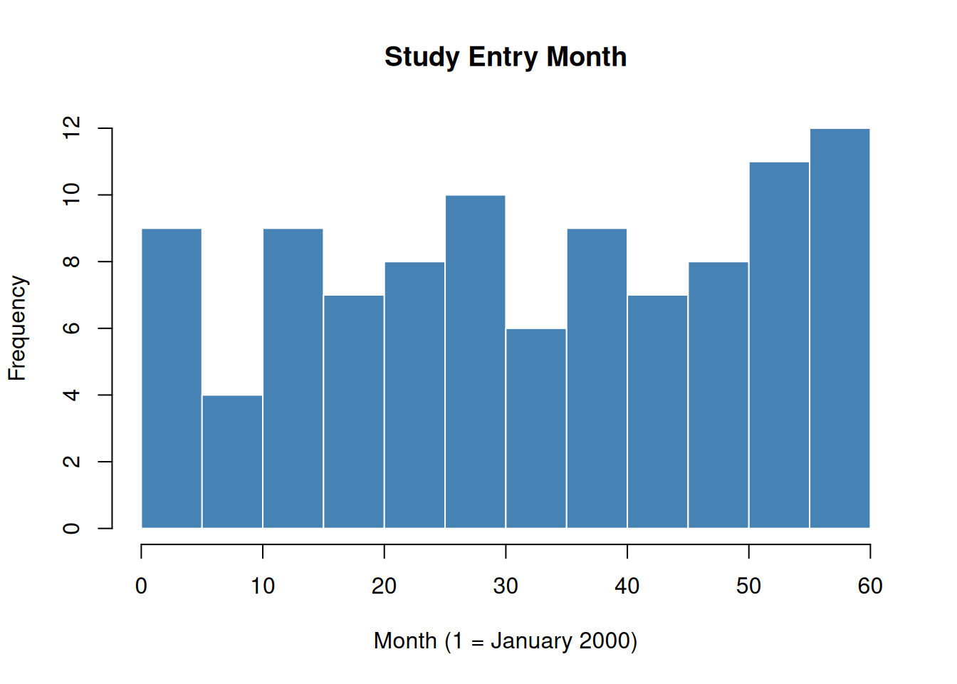
Figure 1: Distribution of study entry months in the simulated cohort.

3 Step 1: Clone and Censor

clone_censor() takes the cohort and mammography event datasets and returns a data frame with two rows per participant — one for each arm.

cloned <- clone_censor(
  cohort,
  screening_mammograms,
  diagnostic_mammograms
)

nrow(cloned) # should be 2 × nrow(cohort)
#> [1] 200
head(cloned[, c("id", "arm", "start_month", "end_month",
                "censor_month", "fup", "died", "bc_died")])
#>   id      arm start_month end_month censor_month fup died bc_died
#> 1  1 STOPBASE          26        38           38  13    0       0
#> 2  2 STOPBASE          33        45           45  13    0       0
#> 3  3 STOPBASE          28        42           42  15    0       0
#> 4  4 STOPBASE           1        12           12  12    0       0
#> 5  5 STOPBASE          17        28           28  12    0       0
#> 6  6 STOPBASE          40        52           52  13    0       0

The key new columns are:

• arm: trial arm ("STOPBASE" or "CONTINUE")
• end_month: final observed month (minimum of death, administrative censoring, and protocol censoring)
• censor_month: month of protocol deviation censoring (NA if not censored for protocol non-adherence)
• fup: follow-up time in months
• died: overall mortality indicator (1 if death caused end of follow-up)
• bc_died: breast cancer mortality indicator

Censoring Patterns by Arm

Because participants in STOPBASE are censored when they get a screening mammogram, annual screeners are censored early in that arm. Conversely, participants in CONTINUE are censored when they go too long without a mammogram, so non-adherers are censored early.

par(mfrow = c(1, 2))

stopbase <- cloned[cloned$arm == "STOPBASE", ]
continue <- cloned[cloned$arm == "CONTINUE", ]

hist(stopbase$fup,
  breaks = 20, main = "STOPBASE",
  xlab = "Follow-up (months)", col = "#E05C4B", border = "white",
  xlim = c(0, 110)
)
hist(continue$fup,
  breaks = 20, main = "CONTINUE",
  xlab = "Follow-up (months)", col = "#4B8FE0", border = "white",
  xlim = c(0, 110)
)
par(mfrow = c(1, 1))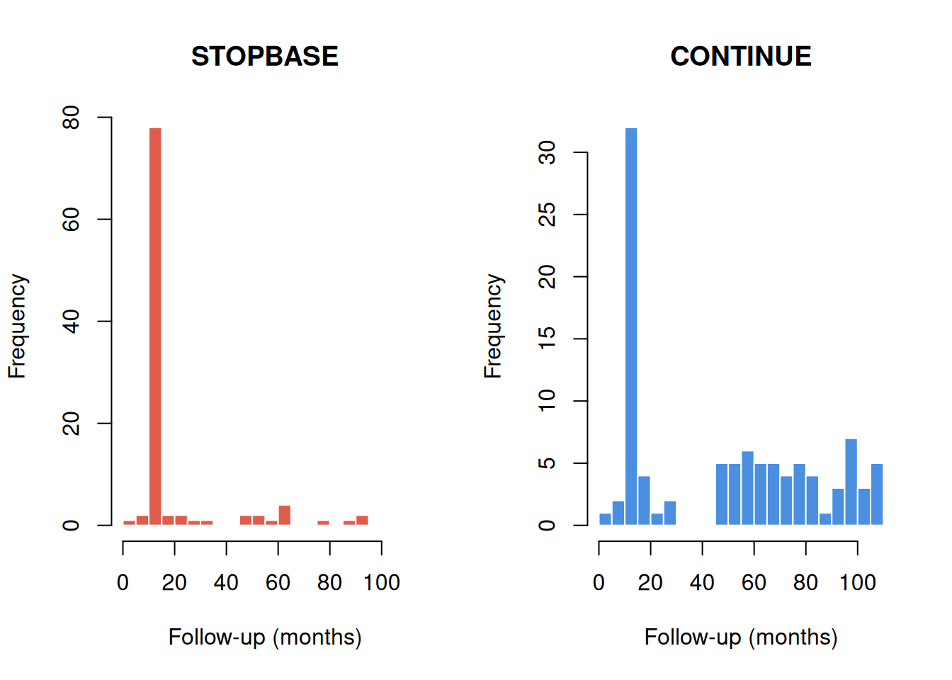

Figure 2: Follow-up time by arm and censoring type.

# Percentage censored for protocol non-adherence in each arm
prop_censored <- tapply(
  !is.na(cloned$censor_month),
  cloned$arm,
  mean
)
round(prop_censored * 100, 1)
#> CONTINUE STOPBASE 
#>       34       90

As expected, most STOPBASE clones are censored (those who continued getting annual mammograms), while only a minority of CONTINUE clones are censored (those who stopped getting mammograms).

4 Step 2: Expand to Long Format

expand_to_long() converts the cloned dataset to one row per participant-arm-month. This format is required for the discrete-time survival models used to estimate the outcome.

long_data <- expand_to_long(cloned)

nrow(long_data) # total person-arm-months
#> [1] 7052
head(long_data)
#>   id      arm month month2 dead_t1 bc_dead_t1 bc_long
#> 1  1 STOPBASE    26      0       0          0       0
#> 2  1 STOPBASE    27      1       0          0       0
#> 3  1 STOPBASE    28      2       0          0       0
#> 4  1 STOPBASE    29      3       0          0       0
#> 5  1 STOPBASE    30      4       0          0       0
#> 6  1 STOPBASE    31      5       0          0       0

The key columns in the long dataset are:

• month: calendar month (1–108)
• month2: months since study entry (0-indexed)
• dead_t1: death in the next interval: 1 = yes, 0 = no, NA = censored
• bc_dead_t1: breast cancer death in the next interval
• bc_long: breast cancer diagnosis flag at this month

# Total events in the long dataset
table(long_data$dead_t1, useNA = "ifany")
#> 
#>    0    1 <NA> 
#> 6852   19  181

Verifying the Long Format

A simple check: the number of observed deaths in the long dataset should equal the number of died == 1 rows in the cloned dataset.

# Deaths in cloned dataset
sum(cloned$died)
#> [1] 19

# Rows with dead_t1 = 1 in long dataset
sum(long_data$dead_t1 == 1L, na.rm = TRUE)
#> [1] 19

5 Step 3: Descriptive Analysis

Before fitting weighted outcome models, it is useful to describe the data and examine crude survival by arm.

We first define a small helper that summarises one arm’s long dataset into a crude cumulative mortality curve. For each month since study entry it counts the deaths, then accumulates them and divides by the number of clones at risk at entry.

crude_cumulative_mortality <- function(arm_long) {
  months <- 0:max(arm_long$month2)

  deaths <- vapply(
    months,
    function(t) sum(arm_long$dead_t1[arm_long$month2 == t] == 1L, na.rm = TRUE),
    numeric(1)
  )
  n_risk <- vapply(
    months,
    function(t) sum(arm_long$month2 == t),
    numeric(1)
  )

  data.frame(
    month2 = months,
    cum_mort = cumsum(deaths) / max(n_risk, 1L)
  )
}

With the computation factored out, plotting the two arms is a short loop over the helper.

arms <- c("STOPBASE", "CONTINUE")
cols <- c("#E05C4B", "#4B8FE0")

plot(NA,
  xlim = c(0, 70), ylim = c(0, 0.15),
  xlab = "Months since study entry",
  ylab = "Cumulative mortality (crude)",
  main = "Crude cumulative mortality by arm"
)

for (j in seq_along(arms)) {
  curve <- crude_cumulative_mortality(long_data[long_data$arm == arms[j], ])
  lines(curve$month2, curve$cum_mort, col = cols[j], lwd = 2)
}

legend("topleft",
  legend = arms, col = cols, lwd = 2, bty = "n"
)

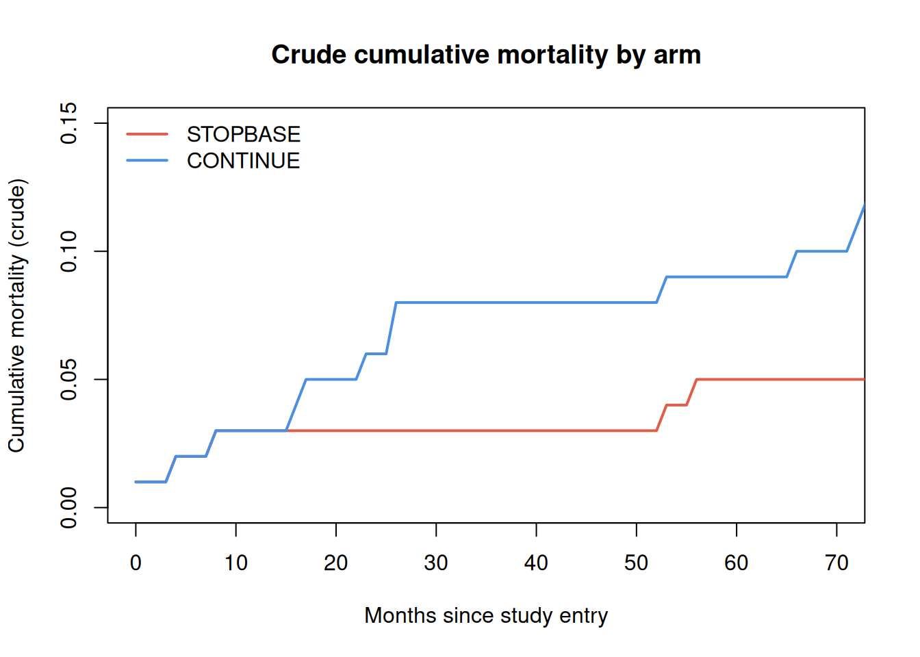
Figure 3: Empirical cumulative mortality by arm (crude, without IPW). Under the null, the two arms should be similar because clones are derived from the same participants.

Note

The crude curves above do not account for the informative censoring introduced by the clone-censor step. The rest of this article applies inverse probability weights (IPW) to correct for the different censoring mechanisms in each arm, then fits the weighted outcome model and bootstraps a confidence interval. See García-Albéniz et al. (2020) for the full analysis on the real cohort.

6 A Larger Simulated Cohort

The 100-participant dataset above is convenient for showing the data structure, but it is too small to fit a stable weighted outcome model: with so few deaths the screening-propensity model separates and the resulting weights are erratic. For the weighted analysis we simulate a larger cohort with simulate_screening_cohort(), which returns the same three linked tables.

The simulation builds in no screening effect on mortality, so the honest expectation is a null result: the two arms should look alike, and the weighted contrast should sit near no difference. What the rest of the article demonstrates is that the machinery runs end to end and recovers that null, not a substantive estimate; a real reproduction needs the Medicare cohort and the paper’s full covariate set.

sim <- simulate_screening_cohort(n = 1000, max_month = 108, seed = 7)

cloned_l <- clone_censor(
  sim$cohort, sim$screening_mammograms, sim$diagnostic_mammograms
)
long_l <- expand_to_long(cloned_l)
long_l <- augment_long_covariates(
  long_l, sim$screening_mammograms, sim$diagnostic_mammograms
)

nrow(long_l) # person-arm-months
#> [1] 73469

7 Step 4: Inverse Probability Weights

fit_screening_propensity() fits the pooled logistic model for the probability of a screening mammogram at each eligible month (the SAS cann17b denominator), and compute_ipw_weights() turns those probabilities into stabilized per-arm weights, truncated at the 99th percentile within each arm.

propensity <- fit_screening_propensity(long_l)
weighted <- compute_ipw_weights(propensity$data, pred_prob_col = "p_scrmammo")

# Stabilized, truncated weights are centered near 1 in both arms
round(t(sapply(split(weighted$wp99, weighted$arm), summary)), 2)
#>          Min. 1st Qu. Median Mean 3rd Qu.  Max.
#> CONTINUE    0       1   1.33 2.10    2.17 15.35
#> STOPBASE    1       1   1.00 5.07   10.15 37.88

8 Step 5: Weighted Outcome Model

fit_outcome_hr() fits the IP-weighted pooled logistic outcome model, with follow-up time entered through a restricted cubic spline and an arm-by-time interaction. The reported odds ratio approximates the hazard ratio for the STOPBASE arm relative to CONTINUE.

hr <- fit_outcome_hr(
  weighted,
  weight_col = "wp99",
  outcome_col = "dead_t1"
)

round(c(OR = hr$or, hr$or_ci), 3)
#>     OR  2.5 % 97.5 % 
#>  0.976  0.669  1.422

As expected under a simulation with no built-in effect, the odds ratio sits near 1 and its confidence interval covers the null.

9 Step 6: Standardized Survival Curves

predict_survival_ipw() applies g-computation to the weighted model, averaging the predicted survival over the cohort to produce a marginal survival curve for each arm.

surv <- predict_survival_ipw(
  weighted,
  weight_col = "wp99",
  outcome_col = "dead_t1"
)

plot(NA,
  xlim = c(0, 72), ylim = c(0.8, 1),
  xlab = "Months since study entry",
  ylab = "Survival probability",
  main = "IP-weighted survival by arm"
)
lines(surv$month, surv$s_continue, col = "#4B8FE0", lwd = 2)
lines(surv$month, surv$s_stopbase, col = "#E05C4B", lwd = 2)
legend("bottomleft",
  legend = c("CONTINUE", "STOPBASE"),
  col = c("#4B8FE0", "#E05C4B"), lwd = 2, bty = "n"
)

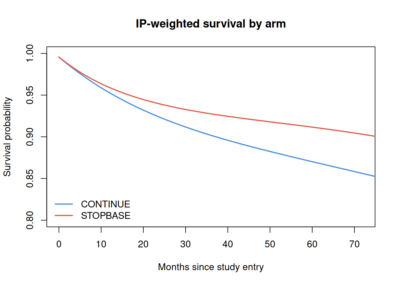
Figure 4: IP-weighted marginal survival by arm. The arms track each other closely, consistent with the null effect built into the simulation.

10 Step 7: Bootstrap Confidence Intervals

bootstrap_ci() resamples participants, recomputes the weights and survival curves on each resample, and returns percentile confidence intervals for the month-by-month survival difference between arms. The number of resamples is kept small here so the article renders quickly; a real analysis uses several hundred.

boot <- bootstrap_ci(
  propensity$data,
  pred_prob_col = "p_scrmammo",
  outcome_col = "dead_t1",
  max_month = 72,
  n_boot = 50,
  seed = 1
)

plot(NA,
  xlim = c(0, 72), ylim = range(c(boot$diff_lo, boot$diff_hi), na.rm = TRUE),
  xlab = "Months since study entry",
  ylab = "Survival difference (CONTINUE - STOPBASE)",
  main = "Bootstrap survival difference with 95% CI"
)
abline(h = 0, col = "grey60", lty = 2)
polygon(
  c(boot$month, rev(boot$month)),
  c(boot$diff_lo, rev(boot$diff_hi)),
  col = "#4B8FE022", border = NA
)
lines(boot$month, boot$diff, col = "#222222", lwd = 2)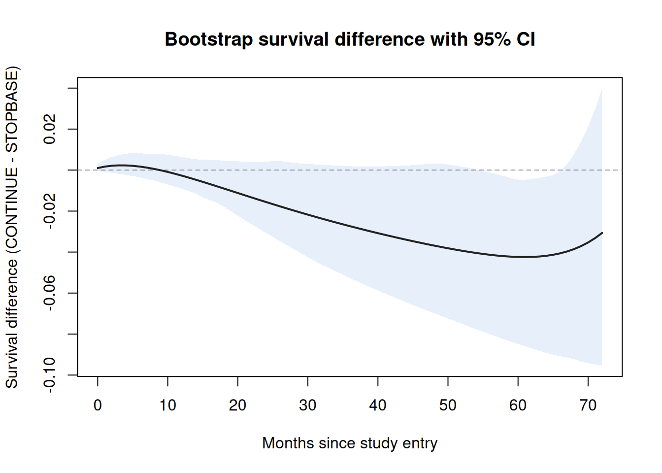

Figure 5: Bootstrap survival difference (CONTINUE minus STOPBASE) with a 95 percent percentile confidence band. The band covers zero throughout, the expected null.

11 Summary

The {ettbc} package implements the full clone-censor-reweight pipeline:

Table 1: Core ettbc functions

Function	Input	Output
simulate_screening_cohort()	cohort size	three linked synthetic tables
clone_censor()	cohort + mammogram events	two rows per participant
expand_to_long()	cloned dataset	one row per participant-arm-month
augment_long_covariates()	long dataset + events	time-varying screening covariates
fit_screening_propensity()	augmented long dataset	screening probabilities
compute_ipw_weights()	long dataset + probabilities	stabilized IPW weights
fit_outcome_hr()	weighted long dataset	arm hazard ratio
predict_survival_ipw()	weighted long dataset	marginal survival curves
bootstrap_ci()	long dataset + probabilities	survival difference with CI

Run on the synthetic cohort, the pipeline recovers the null effect the simulation was built with. Pointed at a real Medicare cohort with the paper’s full covariate set, the same functions reproduce the substantive analysis of García-Albéniz et al. (2020).

The {ettbc} package provides two core functions for the clone-censor step of target trial emulation:

Table 2: Core ettbc functions

Function	Input	Output
clone_censor()	cohort + mammogram events	two rows per participant
expand_to_long()	cloned dataset	one row per participant-arm-month

After running these steps, the long dataset can be used with standard weighted logistic or pooled logistic regression to estimate the intention-to-treat effect of each screening strategy.

12 References

García-Albéniz, Xabier, Hajime Uno, Deepak L Bhatt, Patrick H McArdle, Marshall M Joffe, and Miguel A Hernán. 2020. “Continuation of Annual Screening Mammography and Breast Cancer Mortality in Women Older Than 70 Years: A Prospective Observational Study.” Annals of Internal Medicine 172 (6): 381–89. https://doi.org/10.7326/M18-1199.

Hernán, Miguel A, and James M Robins. 2016. “Using Big Data to Emulate a Target Trial When a Randomized Trial Is Not Available.” American Journal of Epidemiology 183 (8): 758–64. https://doi.org/10.1093/aje/kwv254.