Non-Linear Modeling
Chapter 7 lab handout
Last modified: 2026-09-29
Polynomial Regression and Step Functions
Exercise 1. Load the Wage data with load_data('Wage'). Store the response (wage) as y and the predictor (age) as age.
Exercise 2. Use poly() inside MS() to build a 4th-degree polynomial in age, fit an OLS model of y on this basis, and print the coefficient summary.
Exercise 3. Build a grid age_grid of 100 evenly spaced values spanning the observed range of age, and wrap it in a single-column DataFrame named age_df.
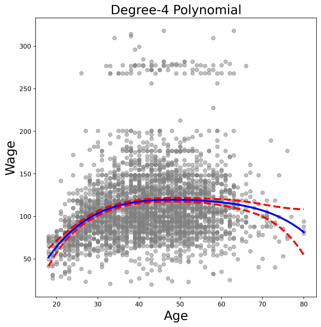
Exercise 4. Write a function plot_wage_fit(age_df, basis, title) that fits OLS on the supplied basis, evaluates it on age_df, and plots the raw data with the fitted curve and its 95% confidence bands.
Exercise 5. Use your helper to plot the degree-4 polynomial fit.
Exercise 6. With polynomial regression we must decide on the degree of the polynomial to use. Fit polynomial models in age of degrees 1 through 5, and use anova_lm() to test which degree is sufficient.
Exercise 7. Repeat the ANOVA, but with a linear term in education included in each model alongside a polynomial in age of degrees 1, 2, 3.
Exercise 8. Now consider predicting whether someone earns more than $250,000 per year. Fit a logistic regression (use sm.GLM with a Binomial family) of wage > 250 on the same 4th-degree polynomial basis in age, and produce a plot of the predicted probability vs. age (with confidence bands and a rug plot).
Solution
| coef | std err | z | P>|z| | |
|---|---|---|---|---|
| intercept | -4.3012 | 0.345 | -12.457 | 0.000 |
| poly(age, degree=4)[0] | 71.9642 | 26.133 | 2.754 | 0.006 |
| poly(age, degree=4)[1] | -85.7729 | 35.929 | -2.387 | 0.017 |
| poly(age, degree=4)[2] | 34.1626 | 19.697 | 1.734 | 0.083 |
| poly(age, degree=4)[3] | -47.4008 | 24.105 | -1.966 | 0.049 |
(The double assignment high_earn = Wage['high_earn'] = y > 250 both binds the local variable high_earn and stores the indicator as a new column on the Wage DataFrame. We’ll re-use that column in Exercises 29 and 30.)
newX = poly_age.transform(age_df)
preds = B.get_prediction(newX)
bands = preds.conf_int(alpha=0.05)

fig, ax = subplots(figsize=(8, 8))
rng = np.random.default_rng(0)
ax.scatter(age +
           0.2 * rng.uniform(size=y.shape[0]),
           np.where(high_earn, 0.198, 0.002),
           fc='gray',
           marker='|')
for val, ls in zip([preds.predicted_mean,
                    bands[:, 0],
                    bands[:, 1]],
                   ['b', 'r--', 'r--']):
    ax.plot(age_df.values, val, ls, linewidth=3)
ax.set_title('Degree-4 Polynomial', fontsize=20)
ax.set_xlabel('Age', fontsize=20)
ax.set_ylim([0, 0.2])
ax.set_ylabel('P(Wage > 250)', fontsize=20);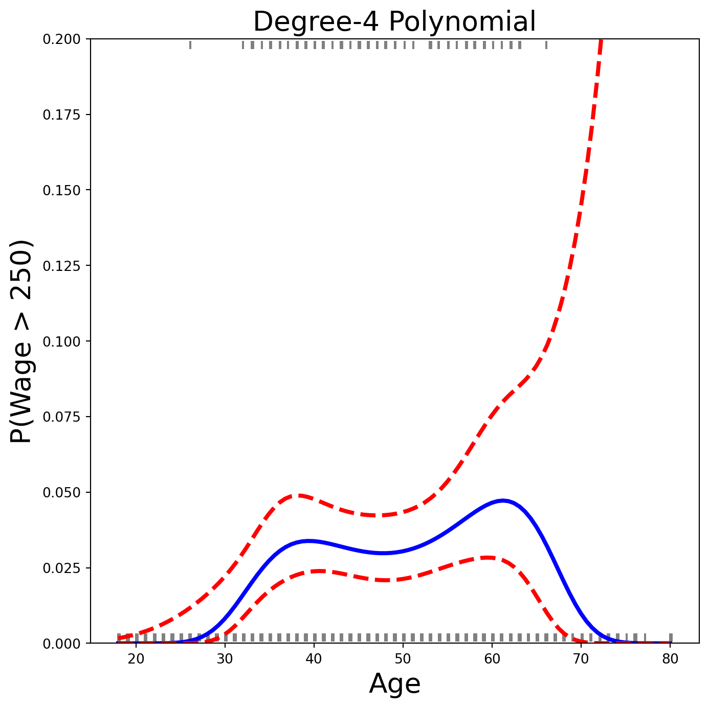
The age values above 250 are shown as gray marks at the top of the plot; those below 250 at the bottom. A small amount of jitter prevents identical-age points from overlapping. This is called a rug plot.
Exercise 9. Fit a step-function regression: discretise age into 4 quantile-based bins with pd.qcut(), build dummy columns with pd.get_dummies(), and fit OLS.
Splines
Exercise 10. Use BSpline() from ISLP.transforms with internal_knots=[25, 40, 60] and intercept=True to build a cubic B-spline basis for age. What shape is the resulting design matrix?
Exercise 11. Now fit a cubic spline regression of wage on age using the helper bs() inside MS(). Pass name='bs(age)' to clean up the column labels in the summary.
Exercise 12. Instead of specifying knots, ask BSpline for df=6. Inspect internal_knots_ to see where the knots ended up.
Exercise 13. B-splines need not be cubic. Fit a degree-0 spline with df=3 and compare the coefficients to your earlier qcut() step-function fit.
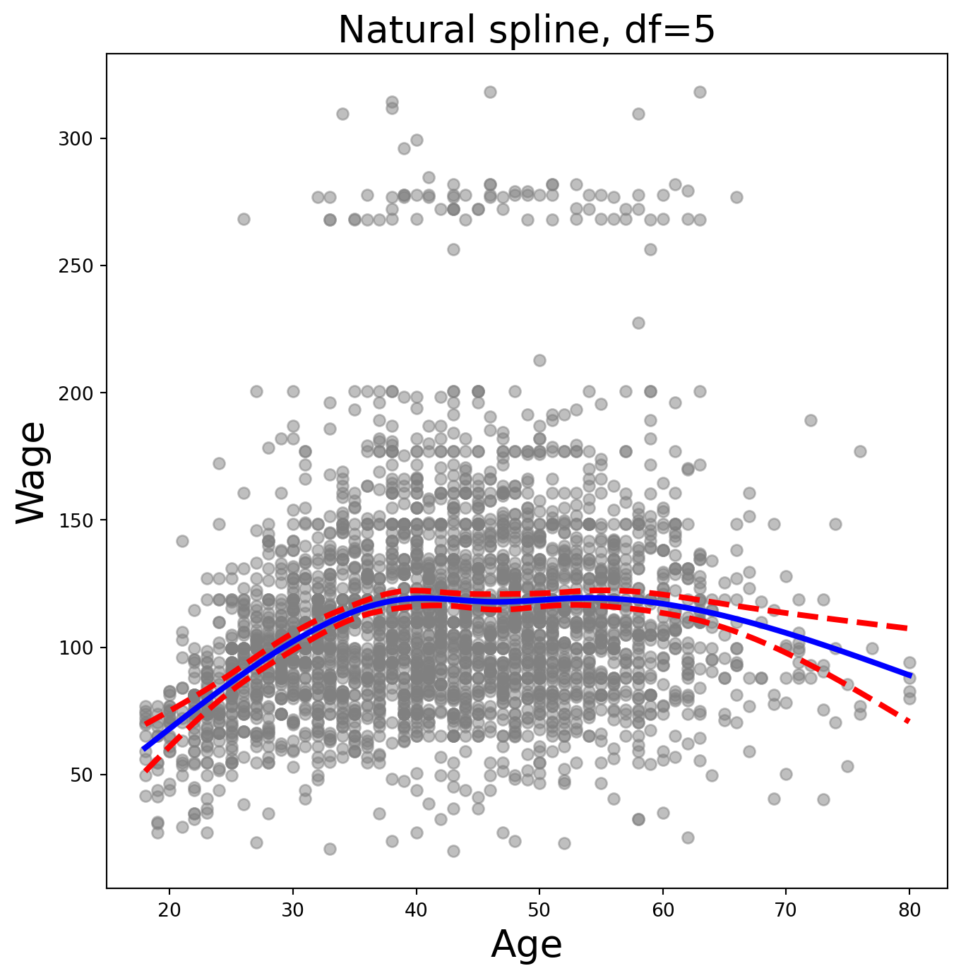
Exercise 14. Fit a natural cubic spline with 5 degrees of freedom using ns(), and plot the fit with plot_wage_fit().
Solution
| coef | std err | t | P>|t| | |
|---|---|---|---|---|
| intercept | 60.4752 | 4.708 | 12.844 | 0.000 |
| ns(age, df=5)[0] | 61.5267 | 4.709 | 13.065 | 0.000 |
| ns(age, df=5)[1] | 55.6912 | 5.717 | 9.741 | 0.000 |
| ns(age, df=5)[2] | 46.8184 | 4.948 | 9.463 | 0.000 |
| ns(age, df=5)[3] | 83.2036 | 11.918 | 6.982 | 0.000 |
| ns(age, df=5)[4] | 6.8770 | 9.484 | 0.725 | 0.468 |
Smoothing Splines and GAMs
Exercise 15. A smoothing spline is a special case of a GAM with squared-error loss and a single feature. Fit LinearGAM(s_gam(0, lam=0.6)) to predict wage from age. (Remember pygam expects a 2-D feature matrix.)
Exercise 16. Investigate how the fit changes with the smoothing parameter. Loop lam over np.logspace(-2, 6, 5) and plot each resulting fit.
Solution
fig, ax = subplots(figsize=(8, 8))
ax.scatter(age, y, facecolor='gray', alpha=0.5)
for lam in np.logspace(-2, 6, 5):
    gam = LinearGAM(s_gam(0, lam=lam)).fit(X_age, y)
    ax.plot(age_grid,
            gam.predict(age_grid),
            label='{:.1e}'.format(lam),
            linewidth=3)
ax.set_xlabel('Age', fontsize=20)
ax.set_ylabel('Wage', fontsize=20);
ax.legend(title=r'$\lambda$');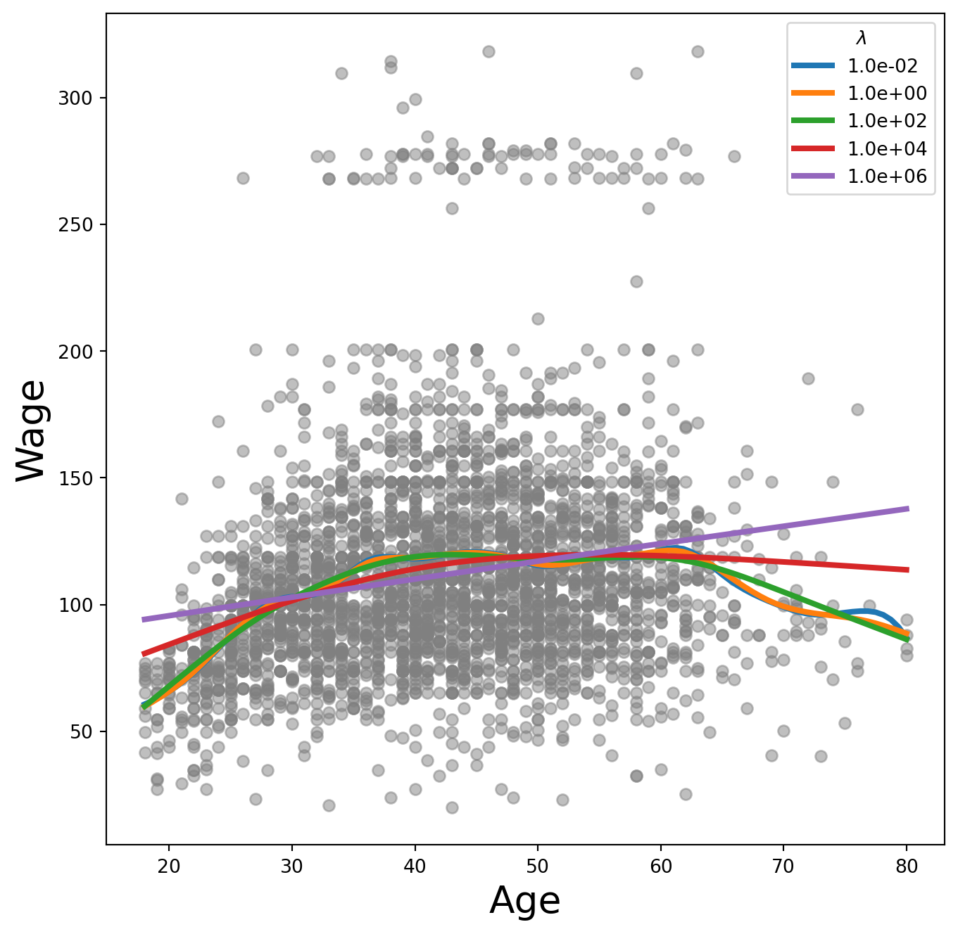
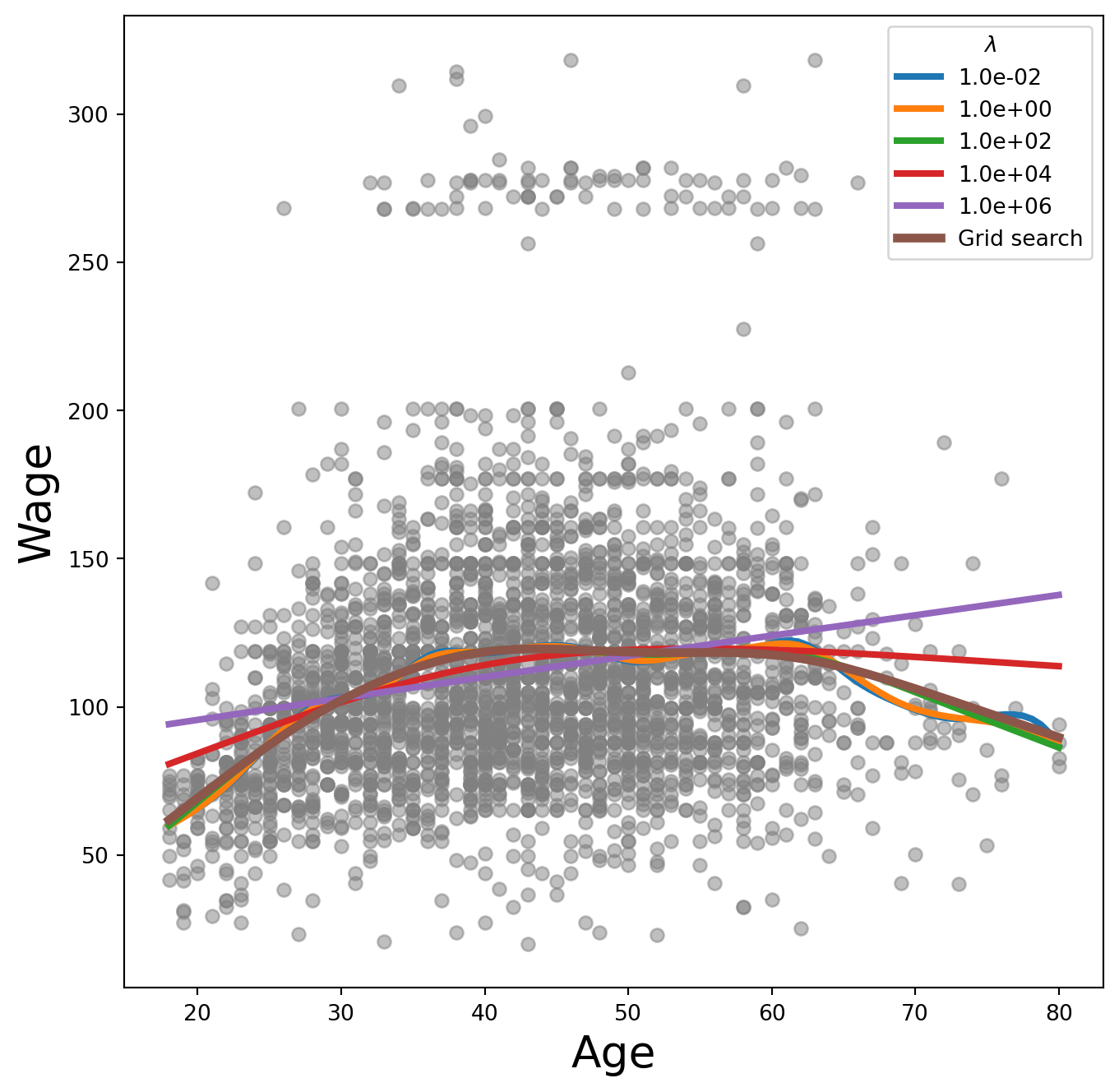
Exercise 17. pygam can search for an optimal smoothing parameter. Reproduce the plot from Exercise 16, call .gridsearch(X_age, y), and add the resulting fit on top.
Solution
fig, ax = subplots(figsize=(8, 8))
ax.scatter(age, y, facecolor='gray', alpha=0.5)
for lam in np.logspace(-2, 6, 5):
    gam = LinearGAM(s_gam(0, lam=lam)).fit(X_age, y)
    ax.plot(age_grid,
            gam.predict(age_grid),
            label='{:.1e}'.format(lam),
            linewidth=3)
gam_opt = gam.gridsearch(X_age, y)
ax.plot(age_grid,
        gam_opt.predict(age_grid),
        label='Grid search',
        linewidth=4)
ax.set_xlabel('Age', fontsize=20)
ax.set_ylabel('Wage', fontsize=20)
ax.legend(title=r'$\lambda$')
fig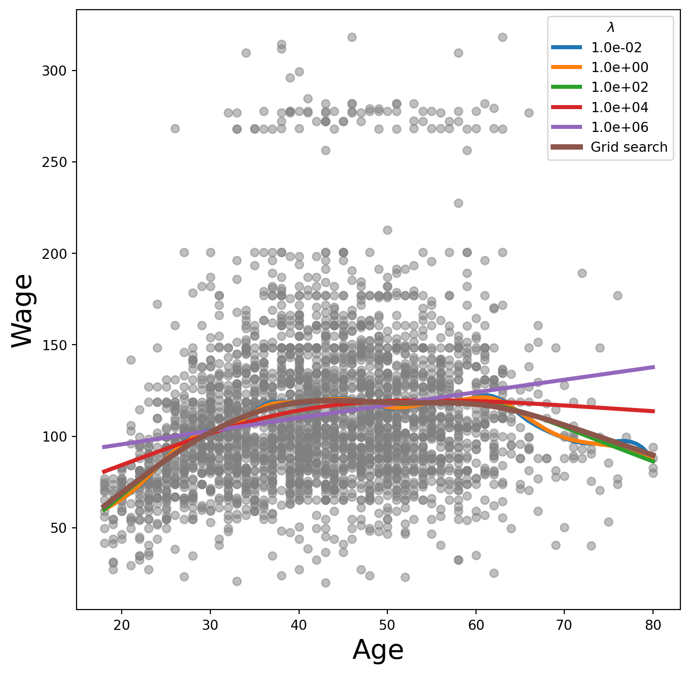
Exercise 18. It’s often more interpretable to specify the effective degrees of freedom than lam. Use approx_lam() from ISLP.pygam to find a lam giving roughly 4 degrees of freedom for the age term, and verify with degrees_of_freedom().
Exercise 19. Now loop over df values [1, 3, 4, 8, 15] (passing df + 1 to approx_lam() to account for the intercept), refit, and plot each.
Solution
fig, ax = subplots(figsize=(8, 8))
ax.scatter(X_age,
           y,
           facecolor='gray',
           alpha=0.3)
for df in [1, 3, 4, 8, 15]:
    lam = approx_lam(X_age, age_term, df + 1)
    age_term.lam = lam
    gam.fit(X_age, y)
    ax.plot(age_grid,
            gam.predict(age_grid),
            label='{:d}'.format(df),
            linewidth=4)
ax.set_xlabel('Age', fontsize=20)
ax.set_ylabel('Wage', fontsize=20);
ax.legend(title='Degrees of freedom');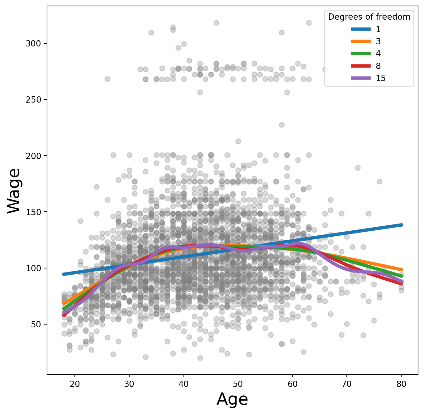
A value of df=1 corresponds to a straight-line fit.
Additive Models with Several Terms
Exercise 20. Build a GAM “by hand”: use natural splines (NaturalSpline) with df=4 for age and df=5 for year, get dummies for education, stack them all into a model matrix X_bh, and fit OLS.
Exercise 21. Construct a partial-dependence plot for age from the by-hand GAM: predict on a matrix where all columns except those for age are held at their column means, and the age columns are swept across age_grid.
Solution
age_grid = np.linspace(age.min(),
                       age.max(),
                       100)
X_age_bh = X_bh.copy()[:100]
X_age_bh[:] = X_bh.mean(0)[None, :]
X_age_bh[:, :4] = ns_age.transform(age_grid)
preds = gam_bh.get_prediction(X_age_bh)
bounds_age = preds.conf_int(alpha=0.05)
partial_age = preds.predicted_mean
center = partial_age.mean()
partial_age -= center
bounds_age -= center
fig, ax = subplots(figsize=(8, 8))
ax.plot(age_grid, partial_age, 'b', linewidth=3)
ax.plot(age_grid, bounds_age[:, 0], 'r--', linewidth=3)
ax.plot(age_grid, bounds_age[:, 1], 'r--', linewidth=3)
ax.set_xlabel('Age')
ax.set_ylabel('Effect on wage')
ax.set_title('Partial dependence of age on wage', fontsize=20);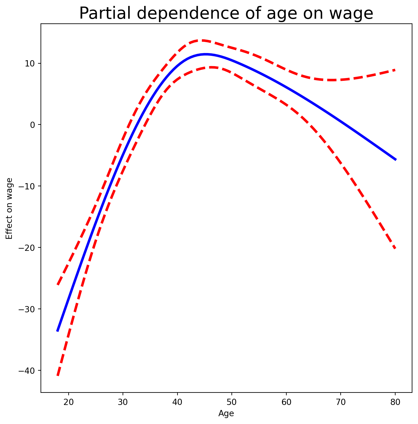
The idea is to create a new prediction matrix in which all but the columns for age are held constant at the training-data means; the four age columns are filled with the natural spline basis evaluated at the 100 values in age_grid.
Exercise 22. Do the same for year.
Solution
year_grid = np.linspace(Wage['year'].min(),
                        Wage['year'].max(),
                        100)
X_year_bh = X_bh.copy()[:100]
X_year_bh[:] = X_bh.mean(0)[None, :]
X_year_bh[:, 4:9] = ns_year.transform(year_grid)
preds = gam_bh.get_prediction(X_year_bh)
bounds_year = preds.conf_int(alpha=0.05)
partial_year = preds.predicted_mean
center = partial_year.mean()
partial_year -= center
bounds_year -= center
fig, ax = subplots(figsize=(8, 8))
ax.plot(year_grid, partial_year, 'b', linewidth=3)
ax.plot(year_grid, bounds_year[:, 0], 'r--', linewidth=3)
ax.plot(year_grid, bounds_year[:, 1], 'r--', linewidth=3)
ax.set_xlabel('Year')
ax.set_ylabel('Effect on wage')
ax.set_title('Partial dependence of year on wage', fontsize=20);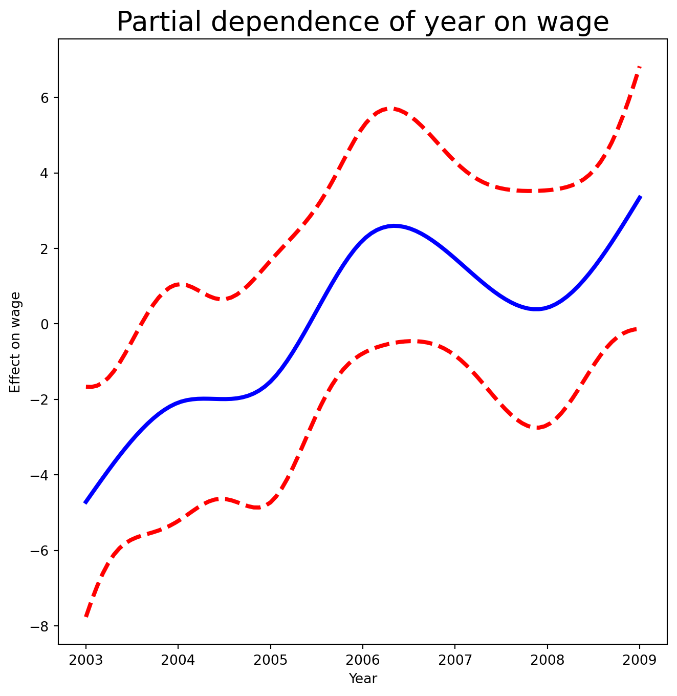
Exercise 23. Now fit the same GAM using smoothing splines via pygam. Build LinearGAM(s_gam(0) + s_gam(1, n_splines=7) + f_gam(2, lam=0)), where f_gam is a factor term for education. (Convert education to numeric codes with .cat.codes.) Then plot the partial dependence for age using plot_gam() from ISLP.pygam.
Solution
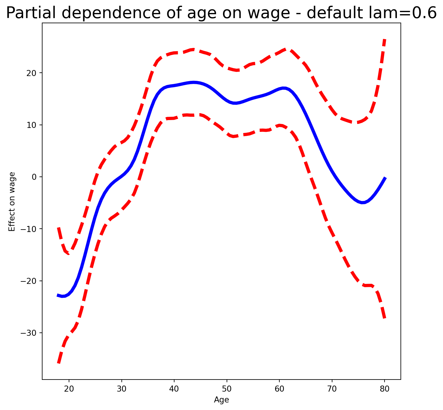
year has only 7 unique values, so we use 7 basis functions. lam=0 on the factor term avoids any shrinkage. The default lam=0.6 for age produces a noticeably wiggly fit.
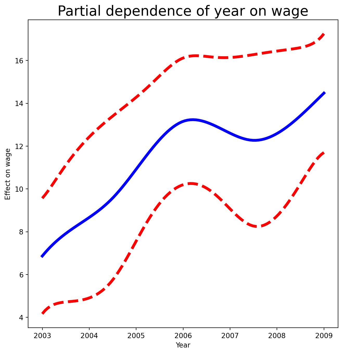
Exercise 24. Re-tune gam_full so that the age and year smoothers each have ~4 degrees of freedom (use approx_lam() with df=4+1), then re-plot the partial dependence for age and for year.
Solution
Note that updating age_term.lam updates gam_full.terms[0] in place.
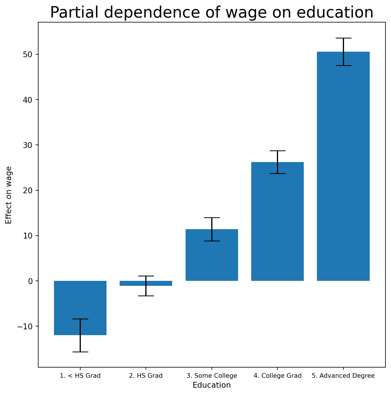
Exercise 25. Plot the partial dependence for education — a categorical term gets a different style of plot, suited to a set of fitted constants per level.
ANOVA Tests for Additive Models
Exercise 26. In all our models, the function of year looks fairly linear. Compare three models by ANOVA: a GAM that excludes year (\(\mathcal{M}_1\)), a GAM that uses a linear term in year (\(\mathcal{M}_2\)), and the full GAM with a smoothing spline in year (\(\mathcal{M}_3\)). What do you conclude?
Exercise 27. Repeat the test for age.
Exercise 28. Print gam_full.summary() and use gam_full.predict() to generate fitted values on the training set.
Exercise 29. Fit a logistic GAM for high_earn (i.e. wage > 250) using LogisticGAM(age_term + l_gam(1, lam=0) + f_gam(2, lam=0)). Plot the partial dependence for education.
Solution
LogisticGAM(callbacks=[Deviance(), Diffs(), Accuracy()],
   fit_intercept=True, max_iter=100,
   terms=s(0) + l(1) + f(2) + intercept, tol=0.0001, verbose=False)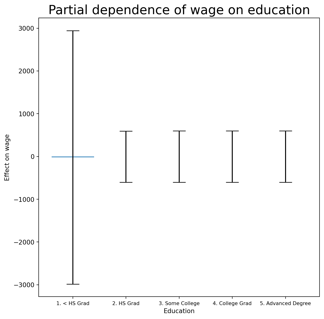
The fit looks flat with very wide error bars on the first category.
Exercise 30. Cross-tabulate high_earn against education. What do you see?
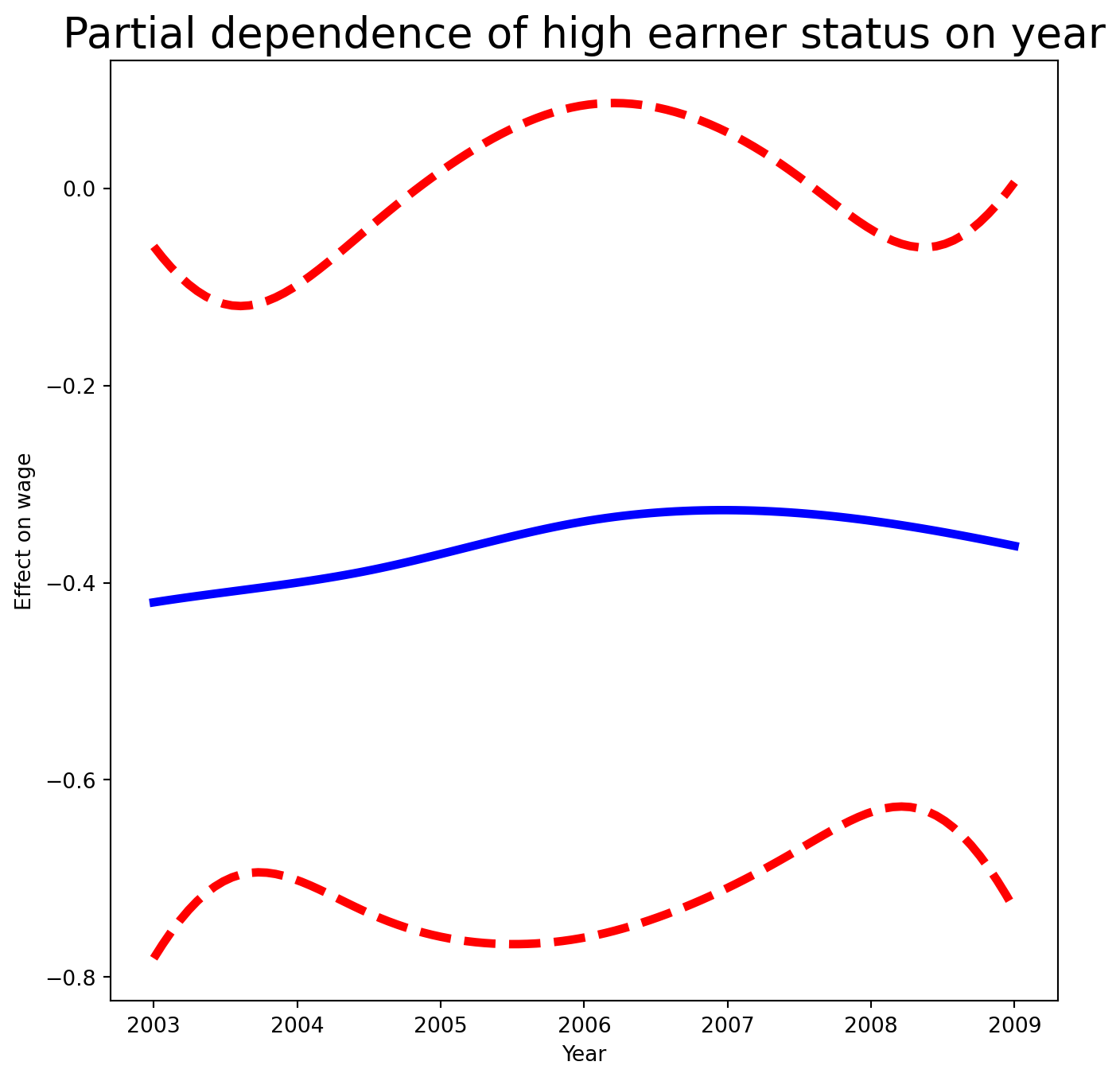
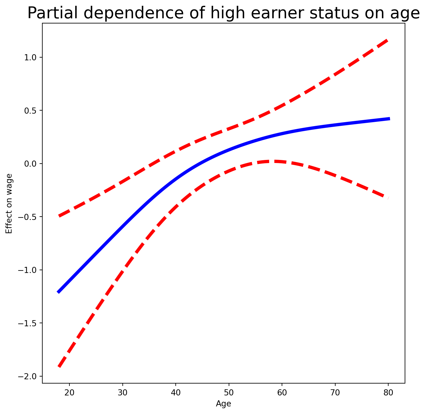
Exercise 31. Refit the logistic GAM excluding observations in the “1. < HS Grad” category, then plot the partial dependence for education, year, and age.
Solution
We subtract 1 from cat.codes to work around a pygam bug — the relabeling has no effect on the fit.
LogisticGAM(callbacks=[Deviance(), Diffs(), Accuracy()],
   fit_intercept=True, max_iter=100,
   terms=s(0) + s(1) + f(2) + intercept, tol=0.0001, verbose=False)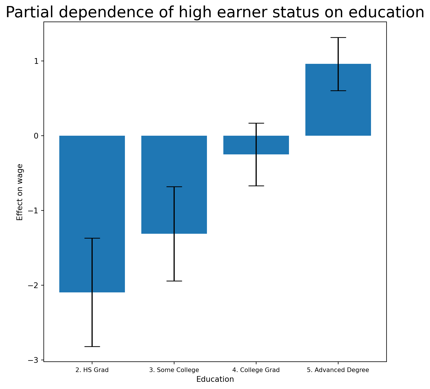
Local Regression
Exercise 32. Finally, use sm.nonparametric.lowess to fit local linear regression models with spans of 0.2 and 0.5, and plot them together. Some implementations of GAMs allow local-regression terms; pygam does not.
Solution
lowess = sm.nonparametric.lowess
fig, ax = subplots(figsize=(8, 8))
ax.scatter(age, y, facecolor='gray', alpha=0.5)
for span in [0.2, 0.5]:
    fitted = lowess(y,
                    age,
                    frac=span,
                    xvals=age_grid)
    ax.plot(age_grid,
            fitted,
            label='{:.1f}'.format(span),
            linewidth=4)
ax.set_xlabel('Age', fontsize=20)
ax.set_ylabel('Wage', fontsize=20);
ax.legend(title='span', fontsize=15);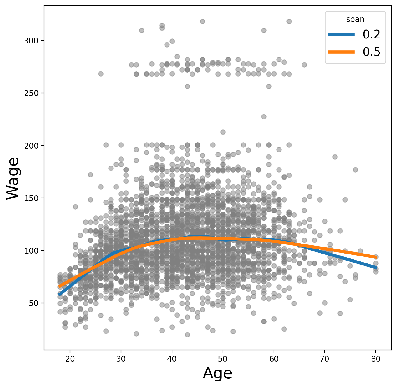
As expected, a span of 0.5 produces a smoother fit than 0.2.