| age | year | education | wage | |
|---|---|---|---|---|
| 0 | 18 | 2006 | 1. < HS Grad | 75.043154 |
| 1 | 24 | 2004 | 4. College Grad | 70.476020 |
| 2 | 45 | 2003 | 3. Some College | 130.982177 |
| 3 | 43 | 2003 | 4. College Grad | 154.685293 |
| 4 | 50 | 2005 | 2. HS Grad | 75.043154 |
Chapter 7 — Moving Beyond Linearity
Introduction to Statistical Learning, 2nd ed.
Last modified: 2026-09-29
Overview
Why move beyond a straight line
Linear regression is interpretable but rigid. Whenever the true relationship between \(Y\) and \(X\) has curvature or thresholds, a straight line trades bias for nothing in return. This chapter keeps the linear- model machinery (OLS, GLM, standard errors) but enriches the model class.
The toolkit
- Polynomial regression — add powers of one predictor.
- Step functions — chop a predictor into bins.
- Regression splines — piecewise polynomials joined at knots.
- Smoothing splines — penalise wiggliness directly.
- Local regression — fit weighted regressions in moving neighbourhoods.
- Generalized additive models (GAMs) — combine the above across many predictors.
Running example: Wage
A US labour-force survey with wage against age, year, education. Used throughout to make every method concrete.
Polynomial Regression
The model
Fit a degree-\(d\) polynomial in one predictor by treating powers of \(X\) as additional columns of the design matrix:
\[Y = \beta_0 + \beta_1 X + \beta_2 X^2 + \cdots + \beta_d X^d + \varepsilon\]
Still linear in the parameters, so OLS theory applies unchanged. The fitted curve is a smooth polynomial of degree \(d\); standard errors at any \(x_0\) come from the usual variance–covariance matrix of \(\hat{\boldsymbol\beta}\).
Choosing the degree
- Visual: plot the fit at several degrees and pick by eye.
- Hypothesis tests (orthogonal polynomials → independent t-tests, or nested-model ANOVA F-tests via
anova_lm). - Cross-validation on test MSE (Chapter 5).
Code
| coef | std err | t | P>|t| | [0.025 | 0.975] | |
|---|---|---|---|---|---|---|
| intercept | 111.7036 | 0.729 | 153.283 | 0.000 | 110.275 | 113.132 |
| poly(age, degree=4)[0] | 447.0679 | 39.915 | 11.201 | 0.000 | 368.805 | 525.331 |
| poly(age, degree=4)[1] | -478.3158 | 39.915 | -11.983 | 0.000 | -556.579 | -400.053 |
| poly(age, degree=4)[2] | 125.5217 | 39.915 | 3.145 | 0.002 | 47.259 | 203.785 |
| poly(age, degree=4)[3] | -77.9112 | 39.915 | -1.952 | 0.051 | -156.174 | 0.352 |
In both languages poly(..., 4) produces a 4-column design matrix using orthogonal polynomials, so individual t-statistics are independent — convenient for choosing the degree.
Try it yourself — Exercises 1–8
From the Ch07 handout:
- Exercise 1. Load the
Wagedata withload_data('Wage'); store the response asyand the predictor asage. - Exercise 2. Use
poly()insideMS()to build a 4th-degree polynomial inage, fit OLS, print the coefficient summary. - Exercise 3. Build a grid
age_gridof 100 evenly spaced values spanning observedage; wrap in a one-column DataFrameage_df. - Exercise 4. Write a helper
plot_wage_fit(age_df, basis, title)that fits OLS onbasis, evaluates it onage_df, and plots data + curve + 95 % bands. - Exercise 5. Use the helper to plot the degree-4 polynomial fit.
- Exercise 6. Fit polynomial models of degrees 1–5 in
age; pick a degree withanova_lm. - Exercise 7. Repeat the ANOVA with a linear
educationterm alongside the polynomial inage. - Exercise 8. Fit a logistic GLM of
wage > 250on the 4th-degree polynomial basis; plot \(P(Y=1)\) vs. age with a rug plot.
Step Functions
The model
Cut \(X\) into \(K+1\) intervals at chosen breakpoints \(c_1 < c_2 < \cdots < c_K\) and fit a separate constant in each interval:
\[Y = \beta_0 + \beta_1 \mathbf 1(c_1 \le X < c_2) + \cdots + \beta_K \mathbf 1(c_K \le X) + \varepsilon\]
The model is piecewise constant — no smoothness across cutpoints. Useful for predictors with a known threshold (e.g. tax brackets) or as a baseline against fancier smoothers.
Code
pd.qcut(x, 4) splits at the 25 / 50 / 75 % quantiles, giving four roughly equal-sized bins. R’s cut(x, 4) instead divides the range of x into four equal-width intervals (which usually leaves the extreme bins much sparser); so the R panel above passes quantile-based breaks explicitly to match Python’s behaviour. In the Python fit each coefficient is the average wage in its bin (no intercept; cell-means parameterisation). The R fit uses the default treatment coding instead — the intercept is the mean of the first bin and the other three coefficients are differences from it.
Try it yourself — Exercise 9
From the Ch07 handout:
- Exercise 9. Fit a step-function regression: discretise
ageinto 4 quantile-based bins withpd.qcut(), build dummy columns withpd.get_dummies(), and fit OLS.
Basis Functions: A Common Framework
The pattern
Polynomial regression and step functions both replace the original \(X\) with a fixed family of basis functions \(b_1(X), b_2(X), \ldots, b_K(X)\) and fit OLS in the new design matrix:
\[Y = \beta_0 + \beta_1 b_1(X) + \cdots + \beta_K b_K(X) + \varepsilon\]
- Polynomial: \(b_k(X) = X^k\).
- Step: \(b_k(X) = \mathbf 1(c_k \le X < c_{k+1})\).
Regression splines use a smarter family — piecewise polynomials joined smoothly at knots — which makes a flexible, local fit possible without exploding the parameter count.
Regression Splines
Piecewise polynomials, smoothly joined
A cubic regression spline is piecewise cubic between knots, with the function value, first derivative, and second derivative continuous at each knot. The total number of free parameters is
\[\underbrace{(K + 3)}_{\text{degrees of freedom}} = (\text{knots}) + (\text{degree}) + 1,\]
equivalently the dimension of the cubic B-spline basis with \(K\) interior knots (no intercept).
Natural cubic splines
A natural cubic spline adds boundary constraints (linear beyond the extreme knots), which trims four parameters off a cubic spline and prevents the wild tail behaviour cubic splines display at the edges of the data. Almost always preferred to plain cubic splines when knots extend to the boundary of \(X\).
Choosing knots and degrees of freedom
- Place knots at quantiles of \(X\) (uniform-by-density).
- Specify degrees of freedom (e.g.
df = 4); the basis constructor picks knot positions for you. - Compare a few df values by cross-validation if it matters.
Code
intercept     56.313841
bs(age)[0]    27.824002
bs(age)[1]    54.062546
bs(age)[2]    65.828391
bs(age)[3]    55.812734
bs(age)[4]    72.131473
bs(age)[5]    14.750876
dtype: float64For a natural spline replace bs(...) with ns(...) in either language — the rest of the workflow is identical.
Try it yourself — Exercises 10–14
From the Ch07 handout:
- Exercise 10. Use
BSpline()withinternal_knots=[25, 40, 60]andintercept=True; check the shape of the design matrix. - Exercise 11. Fit a cubic spline regression with
bs()insideMS(); passname='bs(age)'for cleaner column labels. - Exercise 12. Ask
BSplinefordf=6; inspectinternal_knots_to see where knots ended up. - Exercise 13. Fit a degree-0 spline with
df=3; compare its coefficients to the earlierqcutstep function. - Exercise 14. Fit a natural cubic spline with
df=5vians(); plot the fit withplot_wage_fit().
Smoothing Splines
The motivation
Regression splines need you to pick knots and degrees of freedom. A smoothing spline puts a knot at every observation and controls flexibility through a penalty on roughness:
\[\hat g = \arg\min_{g}\;\sum_{i=1}^n \bigl(y_i - g(x_i)\bigr)^2 \;+\; \lambda \int g''(t)^2\,\mathrm dt\]
- \(\lambda = 0\) — interpolating, infinitely wiggly.
- \(\lambda \to \infty\) — a straight-line OLS fit.
- Intermediate \(\lambda\) — a smooth natural cubic spline.
Effective degrees of freedom
The fit \(\hat{\mathbf y} = \mathbf S_\lambda \mathbf y\) is linear in \(\mathbf y\) via a smoother matrix \(\mathbf S_\lambda\). Its trace gives the effective degrees of freedom:
\[\text{df}_\lambda = \operatorname{tr}(\mathbf S_\lambda).\]
A smoothing spline is often easier to think about by specifying \(\text{df}\) (e.g., “give me an age fit with df \(\approx 4\)”) and letting the software solve for \(\lambda\).
Code
smooth.spline in R finds \(\lambda\) for the requested df directly. In pygam you set \(\lambda\) (lam) explicitly or use ISLP.pygam.approx_lam to translate a desired df into a \(\lambda\).
Try it yourself — Exercises 15–19
From the Ch07 handout:
- Exercise 15. Fit
LinearGAM(s_gam(0, lam=0.6))onage→wage(reshapeageto a 2-D feature matrix). - Exercise 16. Loop
lamovernp.logspace(-2, 6, 5)and plot each resulting fit. - Exercise 17. Reproduce the loop and add a grid-search-optimal fit via
.gridsearch(X_age, y)on top. - Exercise 18. Use
approx_lam()to find alamgiving ≈ 4 effective degrees of freedom; verify withdegrees_of_freedom(). - Exercise 19. Loop
df ∈ {1, 3, 4, 8, 15}(passingdf + 1toapprox_lamfor the intercept), refit, plot.
Local Regression
The idea
For each query point \(x_0\):
- Pick a span (fraction of points to include in the neighbourhood).
- Weight points in \(\mathcal N(x_0)\) by distance from \(x_0\) (e.g., tricubic weights).
- Fit a weighted polynomial (typically degree 0, 1, or 2).
- Predict \(\hat f(x_0)\) from that local model.
Repeat across \(x_0\) to get a smooth curve.
Span vs. smoothness
- Small span — fewer neighbours, lower bias, higher variance.
- Large span — more neighbours, higher bias, lower variance.
Choose by visual inspection or cross-validation. The fitted span has a similar role to \(\lambda\) in smoothing splines.
Code
statsmodels.lowess and R’s loess use slightly different defaults (degree, weighting, robustness) but produce qualitatively similar fits.
Try it yourself — Exercise 32
From the Ch07 handout:
- Exercise 32. Use
sm.nonparametric.lowessto fit local linear regression models with spans of 0.2 and 0.5; plot them together. Notepygamdoes not support local-regression terms inside a GAM.
Generalized Additive Models (GAMs)
The model
Replace the linear sum with a sum of smooth functions, one per predictor:
\[Y = \alpha + f_1(X_1) + f_2(X_2) + \cdots + f_p(X_p) + \varepsilon\]
- Each \(f_j\) can be a polynomial, a regression spline, a smoothing spline, or a step function — different methods can be mixed in the same model.
- Coefficient interpretation becomes “effect of \(X_j\) on \(Y\), holding the other \(X\)’s at their mean”, visualised via partial dependence curves.
Strengths and limits
Strengths
- Captures non-linear effects without giving up the additive interpretability.
- Each \(f_j\) can be tested or constrained separately.
- Inference and ANOVA against nested models works as it does for OLS.
Limits
- Pure additive — no interactions unless you add them explicitly via \(f_{jk}(X_j, X_k)\) terms.
- Effective df grows with the number of smooth terms.
Fitting a GAM with three predictors
LinearGAM(callbacks=[Deviance(), Diffs()], fit_intercept=True,
   max_iter=100, scale=None, terms=s(0) + s(1) + f(2) + intercept,
tol=0.0001, verbose=False)s(...) in both languages is a smoothing-spline term; f_gam in pygam (or a plain factor in R) handles categorical predictors. The mgcv::gam package fits a different smoothness selection algorithm than gam::gam — both are common choices in R.
Partial dependence plots
Visualise the contribution of one predictor while the others are held at their mean (numeric) or summed out (categorical):
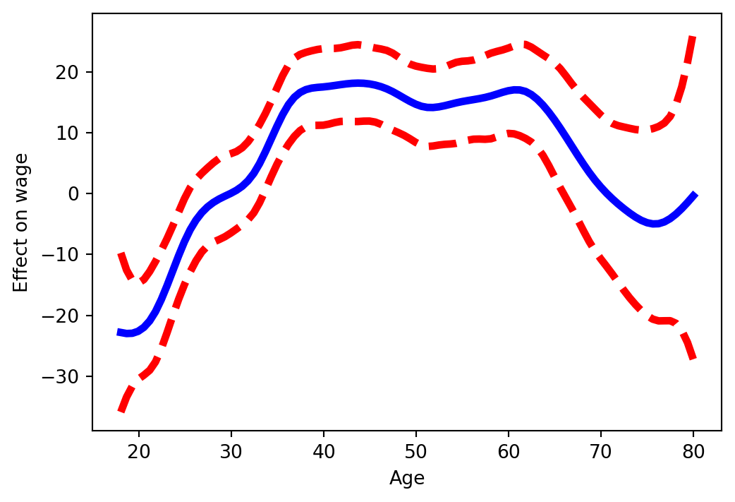
The shape of the partial dependence — flat / linear / hump-shaped / threshold — is what makes GAMs interpretable.
ANOVA-style model comparison
GAMs can be compared by nested ANOVA, just like OLS:
from pygam import l as l_gam
from ISLP.pygam import anova as anova_gam
# gam_no_year: drop year from the feature matrix entirely so the term
# index in the model spec lines up with the column index in X_no_yr.
X_no_yr = np.column_stack([Wage['age'], Wage['education'].cat.codes])
gam_no_year = LinearGAM(s_gam(0) + f_gam(1, lam=0)).fit(X_no_yr, Wage['wage'])
gam_lin_yr  = LinearGAM(s_gam(0) + l_gam(1, lam=0) + f_gam(2, lam=0)).fit(X, Wage['wage'])
anova_gam(gam_no_year, gam_lin_yr, gam)| deviance | df | deviance_diff | df_diff | F | pvalue | |
|---|---|---|---|---|---|---|
| 0 | 105067.669012 | 2980.795583 | NaN | NaN | NaN | NaN |
| 1 | 104791.403410 | 2979.796561 | 276.265602 | 0.999023 | 7.863609 | 0.009898 |
| 2 | 104663.147348 | 2976.214249 | 128.256061 | 3.582312 | 1.018087 | 0.412203 |
GAMs for classification
For a binary outcome (\(Y \in \{0, 1\}\)) extend the additive model to a logistic link:
\[\log\frac{\Pr(Y = 1 \mid X)}{\Pr(Y = 0 \mid X)} = \alpha + \sum_{j=1}^p f_j(X_j)\]
LogisticGAM(callbacks=[Deviance(), Diffs(), Accuracy()],
   fit_intercept=True, max_iter=100,
terms=s(0) + s(1) + f(2) + intercept, tol=0.0001, verbose=False)Try it yourself — Exercises 20–31
From the Ch07 handout:
- Exercise 20. Build a GAM “by hand”:
NaturalSpline(df=4)forage,df=5foryear, dummies foreducation; stack and fit OLS. - Exercise 21. Construct a partial-dependence plot for
agefrom the by-hand GAM. - Exercise 22. Do the same for
year. - Exercise 23. Fit the same model with smoothing splines via
pygam:LinearGAM(s_gam(0) + s_gam(1, n_splines=7) + f_gam(2, lam=0)); plot the age partial dependence. - Exercise 24. Re-tune
gam_fullsoageandyeareach have ≈ 4 df viaapprox_lam(..., df=4+1); re-plot. - Exercise 25. Plot the partial dependence for
education(categorical term). - Exercise 26. ANOVA across three GAMs in
year: excluded vs. linear vs. smooth. What do you conclude? - Exercise 27. Repeat the ANOVA for
age. - Exercise 28. Print
gam_full.summary()and callgam_full.predict()on the training set. - Exercise 29. Fit a logistic GAM for
high_earn(i.e.wage > 250); plot theeducationpartial dependence. - Exercise 30. Crosstab
high_earnagainsteducation— what do you see? - Exercise 31. Refit the logistic GAM excluding the “< HS Grad” category; plot partial dependence for
education,year,age.
Summary
Comparing the tools
| Method | Smoothness | Knot choice | Parametric? | Interactions |
|---|---|---|---|---|
| Polynomial | High order ⇒ wiggly tails | None | Yes | Add product terms |
| Step | None at cutpoints | Manual | Yes | Cross-tabulate factors |
| Regression spline | \(C^2\) at knots | Manual or quantiles | Yes | Tensor product / bs interaction |
| Smoothing spline | Penalty-controlled | All points | Effectively no | Add tensor smooths |
| Local regression | Kernel-controlled | None | No | Multivariate kernel |
| GAM | Per-feature smooth | Per-feature | Hybrid | Add f(X_j, X_k) smooth |
Take-aways
- The methods sit on a spectrum from “rigid, interpretable” to “flexible, hard to read”. Choose by how much you care about each.
- Splines (regression or smoothing) are the workhorse: smooth, local, and computable as standard OLS once a basis is fixed.
- GAMs scale the same ideas to multiple predictors with additive, visualisable effects — the next step before tree-based or neural models.
- Cross-validation (Chapter 5) is the impartial way to compare any of these against linear regression on a given problem.
What’s next
- Chapter 8 — Tree-based methods: decision trees, bagging, random forests, boosting. Different flexibility–interpretability trade-off.
- Chapter 10 — Deep learning: neural networks as another flexible function-fitter, with much higher capacity at the cost of opacity.